Article

A 3D Numerical Study of Interface Effects Influencing Viscous Gravity Currents in a Parabolic Fissure, with Implications for Modeling with 1D Nonlinear Diffusion Equations

by
Eden Furtak-Cole
1,*,†,‡ and
Aleksey S. Telyakovskiy
2,‡
1
Department of Mathematics & Statistics, Utah State University, Logan, UT 84321, USA
2
Department of Mathematics & Statistics, University of Nevada-Reno, Reno, NV 89557, USA
*
Author to whom correspondence should be addressed.
Current address: School of Energy and Environment, City University of Hong Kong, Kowloon Tong, Kowloon, Hong Kong.
These authors contributed equally to this work.
Fluids 2019, 4(2), 97; https://doi.org/10.3390/fluids4020097
Submission received: 15 December 2018 / Revised: 14 May 2019 / Accepted: 22 May 2019 / Published: 28 May 2019
(This article belongs to the Special Issue Advances in Experimental and Computational Rheology)

Abstract

:
Although one-dimensional non-linear diffusion equations are commonly used to model flow dynamics in aquifers and fissures, they disregard multiple effects of real-life flows. Similarity analysis may allow further analytical reduction of these equations, but it is often difficult to provide applicable initial and boundary conditions in practice, or know the magnitude of effects neglected by the 1D model. Furthermore, when multiple simplifying assumptions are made, the sources of discrepancy between modeled and observed data are difficult to identify. We derive one such model of viscous flow in a parabolic fissure from first principals. The parabolic fissure is formed by extruding an upward opening parabola in a horizontal direction. In this setting, permeability is a power law function of height, resulting in a generalized Boussinesq equation. To gauge the effects neglected by this model, 3D Navier-Stokes multiphase flow simulations are conducted for the same geometry. Parameter variations are performed to assess the nature of errors induced by applying the 1D model to a realistic scenario, where the initial and boundary conditions can not be matched exactly. Numerical simulations reveal an undercutting effect observed in laboratory experiments, but not modeled when the Dupuit-Forchheimer assumption is applied. By selectively controlling the effects placed on the free surface in 3D simulations, we are able to demonstrate that free surface slope is the primary driver of the undercutting effect. A consistent lag and overshoot flow regime is observed in the 3D simulations as compared to the 1D model, based on the choice of initial condition. This implies that the undercutting effect is partially induced by the initial condition. Additionally, the presented numerical evidence shows that some of the flow behavior unaccounted for in the 1D model scales with the 1D model parameters.

1. Introduction

Multiple mechanisms can be responsible for the movement of fluids. Gravity currents occur when a difference in the density between two or more fluids induces movement. Applications of this type of movement include both natural [1,2,3,4] and industrial [5,6] settings. Examples of such flows are the propagation of fog banks [7], the phreatic surface in unconfined aquifers [8], C02 injection in brine aquifers [9], and the pouring of molten metal or glass [10]. Gravity currents can be used to model miscible and immiscible flows, which may be laminar or turbulent.
Traditionally, modeling approaches for viscous gravity currents rely on analytical 1D models. In many instances, similarity reductions are possible [8,11]. It is harder to extend such techniques to more realistic 2D and 3D settings. Few solutions [12,13] are available for models using the 2D potential flow equations, which can be reduced to a 1D non-linear diffusion equation by using the Dupuit-Forchheimer (DF) assumption [14]. This assumption allows velocity to be calculated from the slope of the free surface and restricts the velocity to the horizontal direction. This results in a non-divergence free velocity field for incompressible fluids, with the continuity equation imposed on the height of the free surface [15]. For uniform permeability, these assumptions result in the Boussinesq equation with constant coefficients. This equation is commonly used in problems involving the spreading of unconfined groundwater [8,16,17], or flow between parallel plates [1]. Similarity solutions exist for a variety of initial and boundary conditions. For the free spreading of a finite pulse of fluid, Barenblatt [11] constructed a solution using a point mass at initial time. Using a symmetry argument, this solution can be applied to both boundary and initial value problems. Barenblatt’s solution was extended to the fractal dimensions in work of Hayek [18]. Domains with spatially variable permeability can be modeled using the generalized Boussinesq equation, also called the porous medium equation (PME). Similarity solutions exist for cases where the permeability takes the form of a power law in the horizontal or vertical directions [19,20,21,22]. Hele-Shaw cells can be used to study these flows experimentally, with viscous drag serving as a proxy for permeability [23]. Cells constructed in a wedge configuration or with curved walls can be used to validate the PME experimentally. Ciriello et al. [22] constructed similarity solutions to injection problems in horizontal and vertical wedge configurations. For drainage from an initially full aquifer, Zheng et al. [24] developed similarity solutions corresponding to similarly configured experiments. Curved plates resulting in power-law permeability are difficult to manufacture, but have been used for horizontally oriented experiments by Zheng et al. [5], as well as vertical experiments filled with porous media by Longo et al. [25].
Numerical simulations of gravity currents are motivated by the limited scope of similarity solutions, and limitations of the 1D model. Few researchers have conducted numerical simulations of the experiments described above in detail or high dimension. Frolkovič [26] developed a level set solution to the potential flow equations that is applicable to various groundwater problems, including seepage and aquifer drawdown. Numerical modeling efforts specific to the Hele-Shaw cell include Tsay and Hoopes [6] conducting simulations of the free surface of a groundwater mounding problem, Chesnokov and Liapidevskii [27] conducting 2D simulations of viscous fingering, and Bernal and Kindelan [28] simulating 2D non-Newtonian injection. Many authors have pointed out localized discrepancies between experiments and similarity solutions [1,5,22,29], and have offered a variety of case-dependent explanations for the mechanism of error. We have found no examples of attempts to use highly detailed numerical simulations to further investigate these discrepancies. In this work, we pursue this objective.
Numerical investigations of viscous spreading between two non-parallel plates necessitates 3D modeling. For 1D and 2D models, permeability is approximated as a function of space. Our approach is to conduct laminar flow simulations using the 3D Navier-Stokes equations (NSE) with multiphase flow modeled using a volume of fluid (VOF) method. This provides a more direct modeling of the viscous layer that acts in place of permeability, resolves the interface between the fluid phases, and allows for the inclusion of various effects on the interface. To our knowledge, this approach has not yet been applied in this setting. Parabolic prisms provide interesting geometries that are compatible with both 1D analytical solutions and 3D numerical simulations. We derive a flow model for viscous gravity spreading in a parabolic fissure using the DF assumption, resulting in a generalized Boussinesq type equation in Section 2.1. We then numerically investigate different flow scenarios using the 3D model outlined in Section 2.2. This approach allows us to isolate the effects of flow assumptions and parameters in a way that would be intractable using physical experiments. Results of the numerical simulations are outlined in Section 3. From these, mechanisms for the discrepancies between the two models is discussed in Section 4.

2. Governing Equations and Boundary Conditions

2.1. 1D Flow Model

We derive a flow model for a viscous fluid in a parabolic fissure. Consider a fluid element formed by vertically cutting through a parabolic prism, as seen in Figure 1. Conservation of mass dictates that the rate of change of fluid in the elementary volume is equal to the difference in volumetric fluxes through the faces at y and y + d y :
t 0 h v ( y , t ) b ( z ) d z d y = 0 h v ( y , t ) b ( z ) u v ( y , z , t ) d z 0 h v y + d y , t b ( z ) u v ( y + d y , z , t ) d z ,
where the width of the wedge for height z is given by b ( z ) , u v is the fluid speed in the y direction, and h v ( y , t ) is the height of the free surface. We consider only the flux of an incompressible high viscosity fluid (e.g., glycerol), disregarding the flux of gaseous atmosphere being displaced. Neglecting the higher order terms of the Taylor expansion in the second term on the right hand side of Equation (1) yields,
t 0 h v ( y , t ) b ( z ) d z d y = y 0 h v ( y , t ) b ( z ) u v ( y , z , t ) d z d y .
As seen in Figure 1, the parabolic cross section is oriented against gravity in the x-z plane. The equation of the fissure walls in the x-z plane is,
z = ω x 2 ,
for some constant ω > 0 . Then the distance between the walls as a function of height is,
b ( z ) = 2 z ω .
Under the assumption of Poiseuille flow between parallel plates of width b ( z ) for an arbitrary height z, permeability as a power law function of height is obtained:
k ( z ) = b ( z ) 2 12 = z 3 ω .
This permeability results in the Darcy velocity,
u v ( y , z , t ) = z 3 ω ρ g μ h v ( y , t ) y .
Integrating Equation (2), with substitutions for width (4) and Darcy velocity (6), yields
t 4 3 ω h v 3 2 = y 4 15 ω 3 ρ g μ h v 5 2 h v y ,
which further simplifies to,
t h v 3 2 = ρ g 5 ω μ y h v 5 2 h v y .
The change of variables, Υ = h 3 2 , is implemented to obtain a special form of the PME [15]:
t Υ = 2 ρ g 35 ω μ 2 y 2 Υ 7 3 .
We are interested in case of the free spreading of a finite pulse of liquid under the force of gravity, which results in the boundary condition,
Υ ( 0 , t ) = σ t 1 7 / 3 + 1 ,
where σ > 0 for an initially empty fissure [11].
The problem defined by Equations (9) and (10) can be solved by introducing dimensionless similarity variables,
ξ = y ( 1 + β ( m 1 ) ) 1 2 ( a σ ( m 1 ) t 1 + β ( m 1 ) ) 1 2 ,
and
Υ = σ t β H ( ξ ) ,
where ξ ( y , t ) is the similarity variable, H ( ξ ) is a scaling function, m = 7 / 3 is the nonlinear diffusion exponent in the PME, and
a = 2 ρ g 35 ω μ .
The parameter β is the time exponent of the boundary condition, in this case 1 7 / 3 + 1 . Substitution of the similarity variables results in the ordinary differential equation,
d 2 H m ( ξ ) d ξ 2 + ξ 2 d H ( ξ ) d ξ λ H ( ξ ) = 0 ,
where λ = β 1 + β ( m 1 ) , and H ( 0 ) = 1 , H ( ξ 0 ) = 0 . The front position in terms of similarity variables is ξ 0 , and is found in the process of solution. The “mathematician’s pressure” change of variables [15],
H = u 1 m 1 ,
performed on Equation (14) produces an ODE with integer powers:
m m 1 u d 2 u d ξ 2 + m m 1 m m 1 1 d u d ξ 2 + ξ 2 1 m 1 d u d ξ λ u = 0 .
Boundary conditions are given by,
u ( 0 ) = 1 ,
and
u ( ξ 0 ) = 0 .
Equations (16) and (18) can be solved using a Runge-Kutta solver [30], or a power series of the form found in [29]:
u ( ξ ) = n = 0 a n 1 ξ ξ 0 n .

2.2. 3D Flow Model

Flow through the parabolic fissure can be modeled with the incompressible 3D Navier-Stokes equations,
ρ D u D t = p + ρ g + μ Δ u ,
and
· u = 0 ,
where ρ is density, u is velocity, p is pressure, μ is viscosity, and g is the gravity vector. Phases are tracked using a VOF method [31,32]. The indicator function α takes on values in the range of [ 0 , 1 ] and can be interpreted as the fraction of two phase types within a computational cell. For our purposes, 0 denotes air, and 1 denotes a viscous liquid. For any computational cell in the domain, the average fluid properties for density and viscosity are calculated by,
ρ = i ρ i α i ,
and
μ = i μ i α i ,
where α i denotes the volume fraction of phase i. The indicator function evolves under the equation,
α t + · u α + · u c α 1 α = 0 ,
where the counter gradient transport term · u c α 1 α acts as a limiter based on the maximum velocity u c on interface. Surface tension effects are calculated by,
S = γ K α ,
where γ is the surface tension, and K is the curvature · n . S is added to the momentum Equation (20) to obtain,
ρ D u D t = p + ρ g + μ Δ u + γ K α .
This method has been successfully used in applications at a variety of scales [33,34,35,36]. Our use of this method is very conservative, in that the flow is laminar and surface effects are not the main driver of flow. We use the interFoam multiphase flow solver included in the finite volume method toolbox openFOAM [37] for all 3D flow simulations. A hexahedral base mesh was constructed with non-uniform grading decreasing cell size towards the y-z plane and base of the parabola. This mesh was snapped to a 3D parabolic geometry using the snappyHexMesh utility. The parabolic geometry was constructed to the specifications given in Section 2.3. The same mesh was utilized for all simulations, with time-step limiting based on a maximum Courant number of 0.25. With the available computing resources, each simulation required under two days to complete 3 s of simulated time.
Boundary conditions are chosen to mimic a lab experiment, with the top of the parabola open to the atmosphere. For velocity, a no-slip condition,
u = 0 ,
is applied to all solid walls. To allow fluxes of air at the top of the experiment, a zero gradient condition is applied with respect to the patch normal vector:
u n = 0 .
A no-flow pressure condition is applied at the solid walls,
p n = 0 ,
while at the top of the experiment total pressure P t o t is calculated using the gauge pressure p a t m ,
p t o t = p a t m .5 ρ u 2 .
Unless otherwise specified, the indicator function α is fixed at the top of the experiment and zero gradient at solid walls,
α n = 0 .

2.3. Flow Assumptions, Initial Conditions and Parameter Values

The 1D flow model uses the DF assumption, and does not include the effects of air flow, surface tension or contact angle. The 3D model includes a complete velocity field and optional effects at the liquid-gas-wall interface, but requires large amounts of computational power to solve. This is largely due to the aspect ratio of the domain, which requires very small finite volumes between the parabola walls. The parabolic geometry defined by Equation (4) is extruded along the y axis for one meter with a value ω = 2000 . This corresponds to a gap width of x = 2 cm at a maximum height of z = 0.2 m.
An initial condition for the 3D simulation was chosen from the 1D analytical solution using the parameter values in Table 1. The 1D viscosity is held constant at μ = 1.4 Pa ·s for generating the initial condition, though this is effectively varied as part of a (Equation (13)) in the generation of results. Choosing a solution curve from the 1D model at a nonzero starting time is required, as the solution collapses to a singularity at t = 0 s and the height of the solution is above the z 0 , 0.2   m of computational domain at early time. The resulting curve at time t = 0.3   s was chosen as a suitable initial condition containing enough potential energy to produce interesting results. Additional 3D numerical experiments were performed under different values of the parameter a using the same initial condition by exploiting the scaling nature of the similarity solution. After the ODE system Equations (16) and (18) is solved and ξ 0 obtained, the propagation distance y of the 1D solution can be computed as a function of time:
y = ξ 0 a σ ( m 1 ) t 1 + β ( m 1 ) 1 / 2 1 + β ( m 1 ) 1 / 2 .
To compare between 1D and 3D results, the various moments in time from the 1D model to which the initial condition used in 3D simulations corresponds must be calculated. Let the propagation distance of the aforementioned numerical initial condition be y 0 , and a be an alternate parameter value calculated from a 3D simulation parameter set. Then the start time of the numerical initial condition under the parameter set that produced a is,
t 0 = y 0 2 ξ 0 2 1 + β ( m 1 ) a σ ( m 1 ) 1 1 + β ( m 1 ) .

3. Results

In Section 3.1, the models are validated against one another, and the mesh quality of the numerical simulations is shown to be adequate. The mechanisms of discrepancy between the 1D and 3D models is established. Section 3.2 explores the less prominent effects of contact angle and surface tension at the free surface. Additionally, we examine the transition to the similarity flow regime from an initial condition that is not in the similarity solution set. Finally, Section 3.3 examines the behavior of the 3D solution under variations in the parameter a, which is compared against the 1D solution for the analytical initial condition.

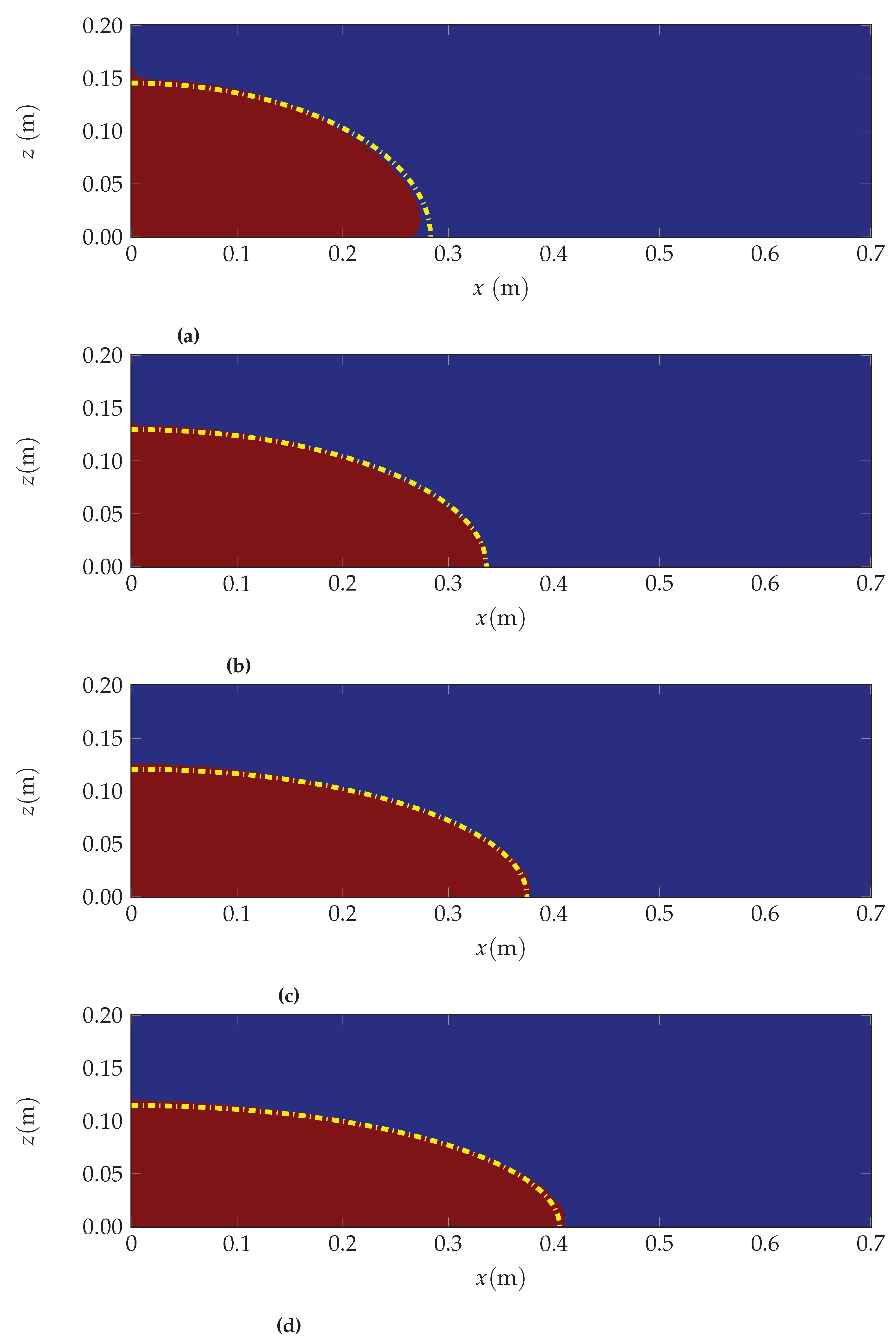
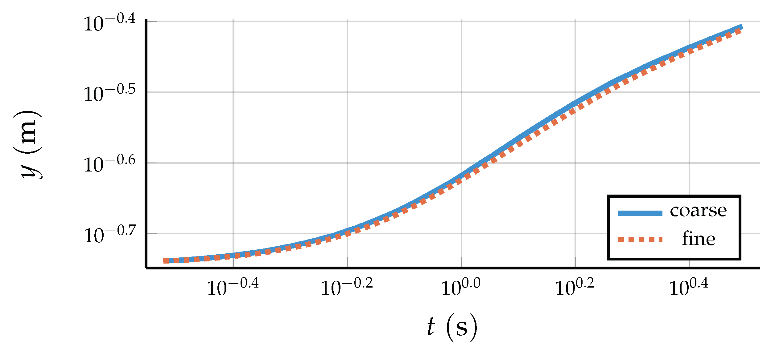
3.1. Profile Comparison and Validation

A comparison between a baseline 3D simulation with γ = 0 and the 1D similarity solution is shown in Figure 2. Excellent agreement is observed between the two models, both in propagation distance and shape. The poorest fit is seen at the earliest time, Figure 2a. The simulated front lags behind the analytical solution at the base of the parabola, and undercutting is observed at the bottom of the advancing front. At later times, the free surface of the 1D analytical solution lags behind the NSE simulation at the “nose” of the advancing front.
The flow profiles observed in this simulation indicate that a steep free surface is responsible for the undercutting observed at early time. The effects of surface tension and contact angle are not included in the simulation used to produce Figure 2, a situation that would be difficult to replicate with experimental techniques.
The 1D flow model presented in Section 2.1 stems from a larger family of nonlinear diffusion equations which have been validated for flow through various fissures. These equations can be derived by substituting an alternative expression for Equation (5). In the case of parallel walls, the resulting Boussinesq equation was experimentally validated by Huppert and Woods [1] using a Hele-Shaw cell and glycerol. Experiments with angled planar walls were validated by Furtak-Cole et al. [29] as well as Ciriello et al. [22] using similar methods. The permeability profile from Equation (5) is bounded on either side by these two classes of experiments, making experimental validation unnecessary.
The interFoam solver presented in Section 2.2 is a type of VOF method [31] which has been used and validated for a variety of applications [33,36]. The cases presented in this paper represent a conservative use of this method, as the maximum Reynolds number is less than one. The role of mesh quality was tested at two levels. Base meshes were constructed with 60 and 80 cells partitioning the width between the parabolic walls. This width is consistent with the x direction shown in the fluid element for the 1D model, see Figure 1. Cell counts in the remaining directions were calculated to maintain a 1-1-1 average aspect ratio. As seen in Figure 3, a consistent rate of propagation was reached at both levels. Propagation distance for the fine mesh lags slightly behind as expected, due to its ability to better resolve the free surface. The finer mesh was used for all simulations presented here. Validation of both 1D and 3D flow models in independent settings, as well as their agreement displayed in Figure 2, implies an acceptable level of accuracy for both solution types.

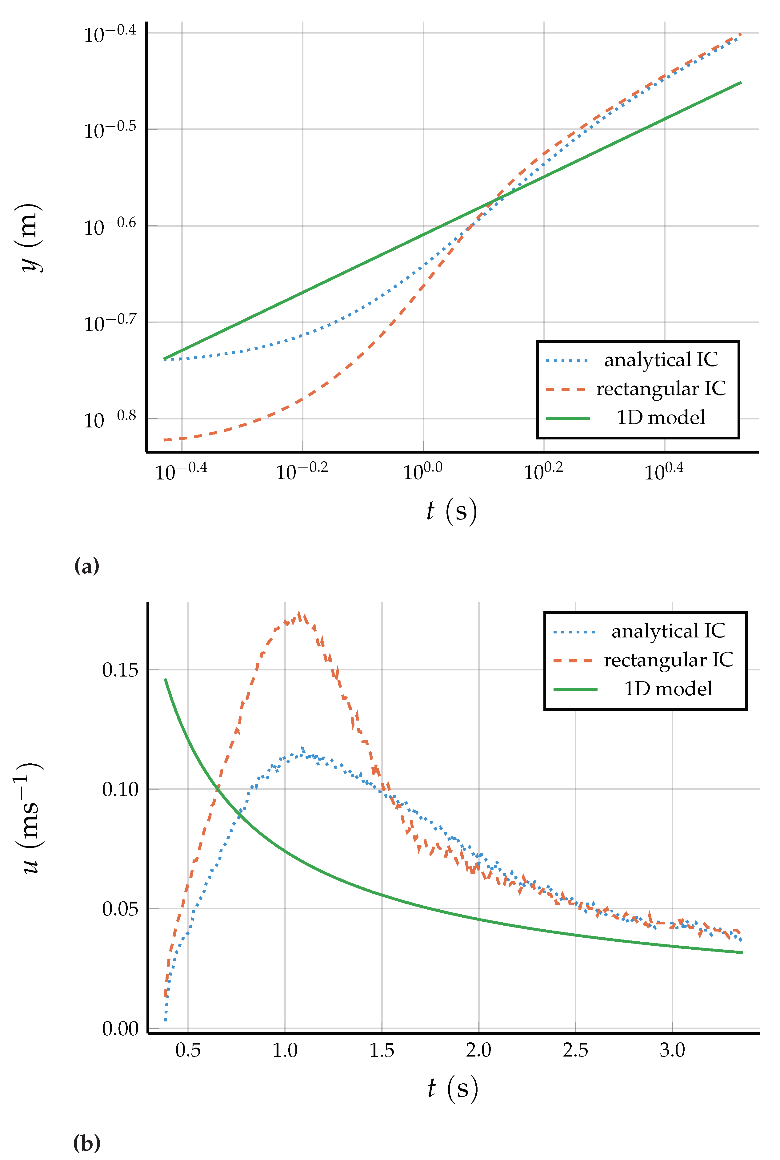
3.2. Effects of Surface Tension, Contact Angle, and Initial Conditions

The similarity solution to the 1D flow problem is a weak, continuous solution. By contrast, the interface resolved by the numerical simulations is double valued at the propagating edge. To quantify this early time behavior observed in experiments and simulations, we measure the height of the undercutting observed in Figure 2a. This is measured vertically from the base of the parabola to the “nose” of the advancing front, where the air-liquid interface is vertical. To further test the assertion that the vertical velocity is primarily responsible for the undercutting behavior, the height of undercutting for simulations with surface tension, dynamic contact angle, and an alternative initial condition are measured. Surface tension for the 3D air-liquid interface is listed in Table 1 and based on the value for glycerol, a viscous fluid commonly used in experiments. A dynamic contact angle θ was modeled using the function,
θ = θ 0 + θ a θ r tanh u w a l l u θ ,
where θ 0 is the static contact angle, u w a l l the speed of the interface tangent the static wall, u θ is a scaling factor, and θ a and θ r are the advancing and receding angles respectively. Given the hypothetical nature of this study and lack of physical data, we arbitrarily choose a neutral parameter set, θ 0 = 90 ° , θ r = 60 ° , θ a = 120 ° , and scaling parameter u θ = 1 .
To perform physical experiments, initial conditions that do not coincide with the similarity solution are often used out of necessity. Such initial conditions have been observed to converge quickly on the similarity solution [5,38]. Numerical experiments offer a previously unobtainable opportunity to compare the convergence of arbitrary initial conditions. A hypothetical mass-conserving initial condition of rectangular cross section was produced by solving,
0 y 1 0 z = 0.18 2 z 2000 d z d y = 3.42548 × 10 4 ,
where the upper limit z = 0.18 was chosen arbitrarily. The value for the right hand side was produced by numerically computing the volume integral defined by the analytically-derived initial condition from the 1D flow model in the parabolic geometry. For practical purposes, such an initial condition could be used in an experiment by setting a lock gate to hold a volume of liquid at the initial time.
Undercut heights for simulations with no interface effects (baseline), contact angle, surface tension, and the alternative rectangular initial condition are shown in Figure 4. Propagation distance and speed for the baseline and rectangular initial condition 3D simulations are compared to the 1D model in Figure 5.

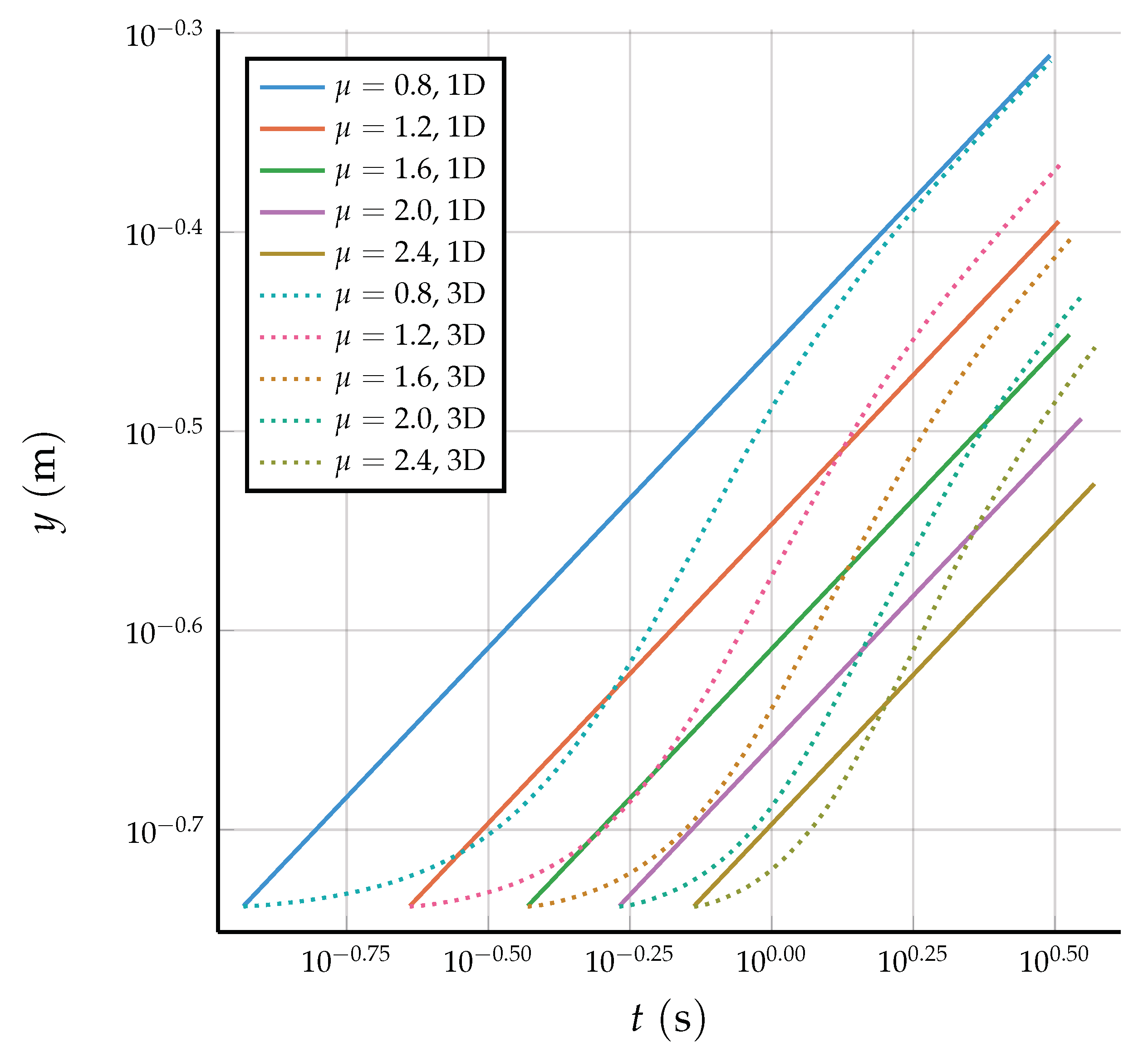
3.3. Scaling Effects

The previously presented results raise the question of whether or not early time inaccuracies of the 1D model can be predicted knowing only the parameters in Equation (9). Given that the coefficients of the right hand side of Equation (9) can be consolidated in a single constant a (Equation (13)), a single parameter can be varied without changing the ode problem given by Equation (14). A natural choice is to vary μ . This allows for all simulations to be performed with the same computational settings, preventing any false comparison of finite volume mesh-induced errors. For the same initial condition, simulations were conducted at the viscosities μ = 0.8 Pa·s, 1.2 Pa·s, 1.6 Pa·s, 2.0 Pa·s, and 2.4 Pa·s. This approach assumes that the parameter values result in a laminar flow, and that at the boundary y = 0 the fixed parameters of Equation (10) guarantee the liquid phase free surfaces change strictly due to gravity. For each simulation, Equation (33) was used to calculate the simulation start time for the single numerical initial condition chosen in Section 2.3, since the same initial profile for different values of μ corresponds to different initial moments in time. Propagation distances are shown in Figure 6, while undercut heights are presented in Figure 7.

4. Discussion

The DF assumption is known to perform poorly for steep free surfaces and the data presented from the numerical simulations make it possible to quantify this deficiency. Use of the DF assumption is often preceded with stipulations such as the ratio of horizontal displacement over height being much larger than one [1]. A smaller ratio results in an increasingly steep free surface with more vertical velocity. Our numerical simulations indicate that vertical velocity components are not only important at the advancing front. Figure 8 shows velocity vectors and their magnitude at a cross section of a baseline simulation as given in Figure 2, after 0.4 s of simulation time. Within the fluid mound, velocities are large only near the interface, while fluid at the lower-left corner is nearly at rest. Primarily vertical velocities are seen at both steep and nearly horizontal segments of the free surface. We calculate continuity error numerically using two control volumes given by a modified version of Equation (1). Here, u ν is given by a surface integral of the spatially variable y component of the velocity in the liquid phase of the 3D simulation seen in Figure 8. Control volumes of 0.01 m width are placed 0.02 m from the left wall and 0.01 m to the left of the advancing front. The time derivative for the volume integral on the left hand side of Equation (1) is approximated with a forward derivative calculated over 0.01 s. The left control volume, positioned at a nearly horizontal free surface, results in a relative continuity error of 0.54%. The right control volume, located on the steep free surface of the advancing front, gives a relative error of 5.06%. In this sense, the 1D model holds well for vertical motions that do not appear near a vertical interface. This indicates that nose formation at the advancing front is at least partially due to a flow regime where fluid “skims” in a direction parallel to the free surface, perhaps better called “overtopping” than “undercutting”. What we have measured as “undercut” is in fact a combination of mechanisms, including viscous drag unaccounted for in the 1D model. In some experiment configurations [1,5] viscous drag is not modeled at the base of the experiment and this effect can not be distinguished from vertical velocity due to the steep free surface. In these cases, it is likely that overtopping is actually compensating viscous drag at the base of experiments, resulting in good agreement between the 1D and experimental results at later times. Indeed, other experiments using vertical wedge configured plates [22,29] experience undercut profiles. No unaccounted drag exists at the base of experiments in these cases, though effects such as surface tension become immense where the plates meet and the cited experiments were performed at an empty initial state with flux boundaries. For the 1D model of a parabolic geometry there is no unaccounted drag at the base of the parabola, though an analogous problem exists: as height decreases to zero, Equation (6) is an increasingly poor approximation of the Darcy velocity because it is based on horizontal width only.
As shown in Figure 4, the magnitude of measured undercutting can be modified by small perturbations in the initial condition or effects acting at the free surface. The rectangular initial condition’s infinite slope dramatically increased the magnitude of undercutting, but the solution rapidly converged on the same trajectory as the analytical initial condition within two seconds. Surface tension caused more extreme long term behavior. The extra force acting parallel to the free surface resists bending, allowing the fluid to override the lowest region of the parabolic wedge for an extended period of time. The Bond number is calculated B o = Δ ρ g L 2 / γ , and represents the interplay between gravitational and surface tension forces. Here, the characteristic length L 2 is determined by the width of the wedge at the height of undercutting in Figure 9a. In the surface tension case, undercut is consistently higher than the baseline case, with the exception of the curves meeting between 1 s and 1.5 s, as seen in the difference plot Figure 9b. This corresponds to large vertical velocities along the leading edge driving the liquid phase downward. Similar residuals are observed at 0.75 s and 2.5 s for an order of magnitude difference in B o , emphasizing the complex relationship between dynamic velocity and surface tension at the interface. The additional simulation using fairly neutral dynamic contact angle parameters shows little change in undercutting as compared to the baseline case. This could undoubtedly be altered by selecting more extreme parameters, however the complicated physics and numerical issues of this topic warrant a separate study. As with the undercutting results, the propagation plots of Figure 5 show the numerical simulations converging on one another rapidly from different initial conditions. While there appears to be discrepancy between the simulations and 1D solution at later times, it is important to note that propagation is measured as the furthest point at the nose of the advancing front. Thus the shape of the profile plays an out-sized role in the measurement of propagation distance, which is not an all-inclusive means of comparing a 3D interface to a 1D solution. More importantly, Figure 5b shows convergence between the propagation velocities for the 3D numerical simulations and 1D model.
Simulations produced for different viscosities show that a period of velocity deficit and overcompensation occurs whenever a simulation is started, as compared to the 1D model solution. This presents a particular problem for experiments where it would be difficult to provide the initial condition with a velocity field from the 1D solution. The starting point of the initial condition relative to the similarity solution and lack of initial velocity are dominant factors in the lack of agreement between the two models. The simulations show increasingly poor convergence to the 1D model the later they are started in time, see Figure 6. In the case of our specific similarity solution, this corresponds to using a higher value of viscosity; a technique often employed to maintain laminar flow in experiments. Initial profiles close to the singular initial condition for the 1D model, and correct initial velocity, are far from the aspect ratio condition that makes the similarity solution applicable. Our results do not establish a general guideline for how severe this effect is; we have not generated a set of different initial profiles corresponding to the same initial moment in time for the different values of viscosity considered here. Still, Figure 6 does show that it would be easy to unknowingly choose a poor combination of initial condition and viscosity (or other parameters that make up a) prior to performing an experiment. Special attention should be paid to this issue.
The dominant role of the initial condition in generating discrepancy is further underscored by plotting the undercut as a function of space in Figure 7b. For each viscosity the time corresponding to the initial condition is different, though each simulation quickly converges to the same trajectory through space. However, the peak value of undercut and its magnitude is shown to shift in space for variations in the value of a. Further analysis reveals a linear relationship between the peak y displacement and the parameter a, shown in Figure 10a. This relationship suggests realistic effects that are not accounted for in the 1D model are still intimately related to the similarity variables governing the 1D solution, and can be predicted as such. Similarly, the magnitude of undercut is plotted against a in Figure 10b, and shows equally linear behavior. The relationships established are purely empirical and further work is needed to understand their mechanism.

5. Conclusions

This paper investigated some of the effects that are neglected by 1D models of viscous gravity spreading under the DF assumption. To have the ability to gauge each effect separately, we conducted highly accurate 3D NSE VOF simulations. Effects neglected by the 1D model were included separately to assess the magnitude of their influence on fluid flow. These effects include vertical components of the flow, surface tension, and contact angle. Each simulation involved the spreading of a finite volume of liquid under the action of gravity.
Undercutting was observed in both the 3D numerical simulations presented here, as well as in previous work by the authors and others. This effect can not be modeled if the DF assumption is used. Undercutting appears when the free surface of the fluid overruns the position of the wetting front at the bottom of the fissure. In this paper, numerical investigations have shown that the primary cause of this effect is vertical velocity induced by a steep free surface. Effects on the free surface may intensify this behavior. Undercutting is strongly influenced by the choice of initial condition. However, late time overall agreement between the two solutions was observed to be very good. This observation is corroborated by previous experimental work. At late times the similarity solution is known to perform well, and the observed height of undercutting takes a small value that changes very slowly for all initial conditions.
To summarize, the placement of the initial condition for numerical experiments relative to the similarity solution parameters produces a wide dilatation in both undercutting and in the position of the advancing front. Initial conditions for numerical simulations that are close quickly converge on each other. Generally, the 1D model predicted the correct speed of propagation, with shortcomings in modeling the shape of the free surface. The DF assumption and associated vertical velocity near steep segments of the free surface are largely responsible for discrepancies between the two models. Effects included at the interface have a secondary role to the above points for the cases considered here.

Author Contributions

Conceptualization, E.F.-C. and A.S.T.; methodology, E.F.-C. and A.S.T.; software, E.F.-C.; validation, E.F.-C.; formal analysis, E.F.-C.; resources, E.F.-C.; writing—original draft preparation, E.F.-C.; writing—review and editing, E.F.-C. and A.S.T.; visualization, E.F.-C.

Funding

This research received no external funding.

Acknowledgments

Eden Furtak-Cole thanks the Utah Center for High Performance Computing for the management of computing resources and access to their technical expertise.

Conflicts of Interest

The authors declare no conflict of interest.

Abbreviations

The following abbreviations are used in this manuscript:
PMEPorous medium equation
DFDupuit-Forcheimer
NSENavier-Stokes equation
VOFVolume of Fluid
BoBond number

References

  1. Huppert, H.E.; Woods, A.W. Gravity-driven flows in porous layers. J. Fluid Mech. 1995, 292, 55–69. [Google Scholar] [CrossRef] [Green Version]
  2. Huppert, H.E. Gravity currents: A personal perspective. J. Fluid Mech. 2006, 554, 299. [Google Scholar] [CrossRef]
  3. Blanchette, F.; Strauss, M.; Meiburg, E.; Kneller, B.; Glinsky, M.E. High-resolution numerical simulations of resuspending gravity currents: Conditions for self-sustainment. J. Geophys. Res. 2005, 110. [Google Scholar] [CrossRef] [Green Version]
  4. Simpson, J.E. Gravity Currents in the Laboratory, Atmosphere, and Ocean. Annu. Rev. Fluid Mech. 1982, 14, 213–234. [Google Scholar] [CrossRef]
  5. Zheng, Z.; Christov, I.; Stone, H. Influence of heterogeneity on second-kind self-similar solutions for viscous gravity currents. J. Fluid Mech. 2014, 747, 218–246. [Google Scholar] [CrossRef]
  6. Tsay, T.S.; Hoopes, J.A. Numerical simulation of ground water mounding and its verification by Hele–Shaw model. Comput. Geosci. 1998, 24, 979–990. [Google Scholar] [CrossRef]
  7. Hrebtov, M.; Hanjalić, K. Numerical Study of Winter Diurnal Convection Over the City of Krasnoyarsk: Effects of Non-freezing River, Undulating Fog and Steam Devils. Bound. Layer Meteorol. 2017, 163, 469–495. [Google Scholar] [CrossRef]
  8. Rupp, D.E.; Selker, J.S. Drainage of a horizontal Boussinesq aquifer with a power law hydraulic conductivity profile. Water Resour. Res. 2005, 41. [Google Scholar] [CrossRef] [Green Version]
  9. Golding, M.J.; Neufeld, J.A.; Hesse, M.A.; Huppert, H.E. Two-phase gravity currents in porous media. J. Fluid Mech. 2011, 678, 248–270. [Google Scholar] [CrossRef]
  10. Naaim, M.; Gurer, I. Two-phase Numerical Model of Powder Avalanche Theory and Application. Nat. Hazards 1998, 17, 129–145. [Google Scholar] [CrossRef]
  11. Barenblatt, G.I. Scaling; Cambridge University Press: Cambridge, UK, 2003. [Google Scholar]
  12. Polubarinova-Kochina, P.Y. Theory of Groundwater Movement; Princeton University Press: Princeton, NJ, USA, 1962. [Google Scholar]
  13. Longo, S.; Di Federico, V. Axisymmetric gravity currents within porous media: First order solution and experimental validation. J. Hydrol. 2014, 519, 238–247. [Google Scholar] [CrossRef]
  14. McWhorter, D.B.; Sunada, D.K. Ground-Water Hydrology and Hydraulics; Water Resources Publications: Highlands Ranch, CO, USA, 1977. [Google Scholar]
  15. Vazquez, J.L. The Porous Medium Equation, Mathematical Theory; Oxford University Press: Oxford, UK, 2007. [Google Scholar]
  16. Lockington, D.A.; Parlange, J.Y.; Parlange, M.B.; Selker, J. Similarity solution of the Boussinesq equation. Adv. Water Resour. 2000, 23, 725–729. [Google Scholar] [CrossRef] [Green Version]
  17. Telyakovskiy, A.S.; Braga, G.A.; Kurita, S.; Mortensen, J. On a power series solution to the Boussinesq equation. Adv. Water Resour. 2010, 33, 1128–1129. [Google Scholar] [CrossRef]
  18. Hayek, M. An exact solution for a nonlinear diffusion equation in a radially symmetric inhomogeneous medium. Comput. Math. Appl. 2014, 68, 1751–1757. [Google Scholar] [CrossRef]
  19. Barenblatt, G.I. On Some Unsteady-State Movements of Liquid and Gas in Porous Medium. Prikl. Mat. Mekh. 1952, 16, 67–78. (In Russian) [Google Scholar]
  20. Barenblatt, G.I. On some problems of unsteady filtration. Izv. AN SSSR 1954, 6, 97–110. (In Russian) [Google Scholar]
  21. Olsen, J.S.; Telyakovskiy, A.S. Polynomial approximate solutions of a generalized Boussinesq equation. Water Resour. Res. 2013, 49, 3049–3053. [Google Scholar] [CrossRef]
  22. Ciriello, V.; Longo, S.; Chiapponi, L.; Di Federico, V. Porous gravity currents: A survey to determine the joint influence of fluid rheology and variations of medium properties. Adv. Water Resour. 2016, 92, 105–115. [Google Scholar] [CrossRef]
  23. Helmig, R. Multiphase Flow and Transport Processes in the Subsurface: A Contribution to the Modeling of Hydrosystems; Springer: Berlin/Heidelberg, Germany, 1997. [Google Scholar]
  24. Zheng, Z.; Soh, B.; Huppert, H.E.; Stone, H.A. Fluid drainage from the edge of a porous reservoir. J. Fluid Mech. 2013, 718, 558–568. [Google Scholar] [CrossRef] [Green Version]
  25. Longo, S.; Ciriello, V.; Chiapponi, L.; Di Federico, V. Combined effect of rheology and confining boundaries on spreading of gravity currents in porous media. Adv. Water Resour. 2015, 79, 140–152. [Google Scholar] [CrossRef]
  26. Frolkovič, P. Application of level set method for groundwater flow with moving boundary. Adv. Water Resour. 2012, 47, 56–66. [Google Scholar] [CrossRef]
  27. Chesnokov, A.; Liapidevskii, V. Viscosity-stratified flow in a Hele–Shaw cell. Int. J. Non Linear Mech. 2017, 89, 168–176. [Google Scholar] [CrossRef]
  28. Bernal, F.; Kindelan, M. RBF meshless modeling of non-Newtonian Hele–Shaw flow. Eng. Anal. Bound. Elem. 2007, 31, 863–874. [Google Scholar] [CrossRef]
  29. Furtak-Cole, E.; Telyakovskiy, A.S.; Cooper, C.A. A series solution for horizontal infiltration in an initially dry aquifer. Adv. Water Resour. 2018, 116, 145–152. [Google Scholar] [CrossRef]
  30. Shampine, L.F. Some Singular Concentration Dependent Diffusion Problems. J. Appl. Math. Mech. 1973, 53, 421–422. [Google Scholar] [CrossRef]
  31. Hirt, C.W.; Nichols, B.D. Volume of fluid (VOF) method for the dynamics of free boundaries. J. Comput. Phys. 1981, 39, 201–225. [Google Scholar] [CrossRef]
  32. Darwish, M.; Moukalled, F. Convective Schemes for Capturing Interfaces of Free-Surface Flows on Unstructured Grids. Numer. Heat Transf. B Fund 2006, 49, 19–42. [Google Scholar] [CrossRef]
  33. Deshpande, S.S.; Anumolu, L.; Trujillo, M.F. Evaluating the performance of the two-phase flow solver interFoam. Comput. Sci. Discov. 2012, 5, 014016. [Google Scholar] [CrossRef]
  34. Yin, X.; Zarikos, I.; Karadimitriou, N.; Raoof, A.; Hassanizadeh, S. Direct simulations of two-phase flow experiments of different geometry complexities using Volume-of-Fluid (VOF) method. Chem. Eng. Sci. 2019, 195, 820–827. [Google Scholar] [CrossRef]
  35. Issakhov, A.; Imanberdiyeva, M. Numerical simulation of the movement of water surface of dam break flow by VOF methods for various obstacles. Int. J. Heat Mass Transf. 2019, 136, 1030–1051. [Google Scholar] [CrossRef]
  36. Duguay, J.; Lacey, R.; Gaucher, J. A case study of a pool and weir fishway modeled with OpenFOAM and FLOW-3D. Ecol. Eng. 2017, 103, 31–42. [Google Scholar] [CrossRef]
  37. Weller, H.G.; Tabor, G.; Jasak, H.; Fureby, C. A tensorial approach to computational continuum mechanics using object-oriented techniques. Comput. Phys. 1998, 12, 620. [Google Scholar] [CrossRef]
  38. Hesse, M.; Tchelepi, H.; Cantwel, B.J.; Orr, F.M., Jr. Gravity currents in horizontal porous layers: Transition from early to late self-similarity. J. Fluid Mech. 2007, 577, 363–383. [Google Scholar] [CrossRef]
Figure 1. A fluid element within the parabolic Hele-Shaw cell. The cross-sectional width is denoted b ( z ) , and the flux through the element is u ν .
Fluids 04 00097 g001
Figure 2. Comparisons in the y z plane cross section between the NSE simulation and 1D flow model at (a) 1.3 s, (b) 2.3 s, (c) 3.3 s, and (d) 4.3 s. Red represents glycerol in the simulation results, the yellow dotted line is the free surface from the 1D model.
Fluids 04 00097 g002
Figure 3. Front propagation for identical simulations of viscosity μ = 1.4 with two mesh partitions. The coarse corresponds to 60 cells in the x-direction, while the fine has 80.
Fluids 04 00097 g003
Figure 4. Height of undercutting plotted from its maximum as a function of time. The removal of surface tension results in a profile with less undercutting.
Fluids 04 00097 g004
Figure 5. (a) Front propagation for two baseline 3D simulations and the 1D flow model. The analytical and rectangular initial conditions used have the same mass. (b) Propagation velocity u for the same 3D simulations and 1D model. A lag is observed as momentum builds, and results in overshoot at the nose of the advancing front where distance is measured in (a). Numerical calculation of front velocity reveals convergence in (b).
Fluids 04 00097 g005
Figure 6. An overlay of propagation distances for the 1D model and 3D simulations at various viscosities.
Fluids 04 00097 g006
Figure 7. (a) Undercut heights plotted from peak value as a function of time. Shifting of the peaks is largely due to the start times calculated by Equation (33). (b) Undercut heights plotted from peak value as a function of space. In all cases, only μ is varied and no interfacial effects are present.
Fluids 04 00097 g007
Figure 8. Velocity vectors from the cross section of a 3D simulation. Vectors are scaled by magnitude and colored by vertical component, with blue denoting downward velocity and red upward velocity. The background is colored by velocity magnitude, with blue denoting zero and red denoting high velocity. Strong downward motions are seen within the fluid mound (left), while strong updrafts are seen in the air being displaced by the advancing front (center right). The midpoint along the arc length of the interface is characterized by a nearly stagnant zone, where velocity changes from negative at left to positive at right with respect to the interface outward normal vector.
Fluids 04 00097 g008
Figure 9. (a) Bond number calculated at the height of undercut for the surface tension case. (b) Difference between the surface tension and baseline cases. Bond number and differences from simulations presented in Figure 4. The lack of correlation between B o and the difference occurs as velocity builds from the initial condition.
Fluids 04 00097 g009
Figure 10. (a) A strong linear relationship is observed between the peak distance y and the parameter a, with a standard error of 0.0031 m. (b) Peak undercut height as a function of μ . Standard error for the linear fit is 0.0018 m. Both are measured from the baseline case when no modeled interface effects are present.
Fluids 04 00097 g010
Table 1. Parameter values for the 1D and 3D models.
1D ParameterValue3D ParameterValue
σ 0.06   m --
ρ 1261 kg·m−3 ρ l i q u i d 1261 kg·m−3
μ 0.88–2.4 Pa·s μ l i q u i d 0.8–2.4 Pa·s
g9.8 m·s−2g9.8 m·s−2
ω 2000--
-- ρ a i r 1 kg·m−3
-- μ a i r 1.48 × 10⁻⁵ Pa·s
-- γ 0.0634 N·m−1

