An Experimental and Computational Study on Inverted Flag Dynamics for Simultaneous Wind–Solar Energy Harvesting

Abstract

This paper presents results from experiments and simplified numerical simulations on the flow-induced dynamics and power generation of inverted flags that combine flexible piezoelectric strips with photovoltaic cells to simultaneously harvest kinetic wind energy and solar radiant energy. Experiments were conducted in a wind tunnel under controlled wind excitation and light exposure, focusing in particular on the dynamics and power generation of the inverted flag harvester. Numerical simulations were carried out using a lattice-Boltzmann fluid solver coupled with a finite element structural solver via the immersed-boundary method, focusing in particular on minimizing the simulation run time. The power generated during the tests shows that the proposed inverted flag harvester is a promising concept, capable of producing enough power (on the order of 1 mW) to supply low-power electronic devices in a range of applications where distributed power generation is needed. Notwithstanding key simplifications implemented in the numerical model to achieve a fast execution, simulations and measurements are in good agreement, confirming that the lattice-Boltzmann method is a viable and time-effective alternative to classic Navier–Stokes-based solvers when dealing with strongly coupled fluid–structure interaction problems characterized by large structural displacements.

1. Introduction

Energy harvesting is the process by which ambient background energy (e.g., kinetic energy from wind/water flow or motion, solar radiation, structural vibration, temperature or salinity gradients, electromagnetic energy) is recovered to supply small-scale low-power (microwatt to milliwatt power range) electronic devices such as sensors, data-loggers, and data-transmitters for use in distributed sensing, equipment/process monitoring, smart city, and Internet of things applications [1,2,3,4,5,6]. Piezoelectric materials, in particular, were quite extensively investigated for harvesting energy from structural and flow-induced movement or vibration [7,8,9,10,11,12,13,14,15,16,17,18,19]. Piezoelectric harvesters typically comprise a structural element realized with a piezoelectric material (or bonded with a piezoelectric patch) that is either connected to a vibrating or moving structure, or exposed to fluid flow in such a way that flow-induced vibration or motion takes place. The structural or flow-induced vibration/motion periodically bends the piezoelectric material, which in turn converts mechanical strain into electric energy. Piezoelectric polymers such as polyvinylidene fluoride (PVDF) are highly flexible, low-cost, lightweight, and they can endure cyclic mechanical loads; therefore, they are particularly suited for energy harvesting [20]. To achieve optimal power output, PVDF elements should undergo large-amplitude deformations and sustained periodic motion, such as a large-amplitude limit-cycle oscillation. A large amplitude deformation, in fact, yields large strain levels and, therefore, large electrical output. A continuous periodic motion, on the other hand, assures a sustained electrical output without interruptions.

Several configurations were explored for energy harvesting from wind excitation. Among these, the inverted flag is a particularly attractive one for wind energy harvesting with PVDF elements. Being free to flap at the upstream leading edge and fixed at the downstream trailing edge, the inverted flag is in fact inherently more unstable than the upstream-clamped regular flag. As a result, flapping can be sustained with comparatively lower wind speeds, and the flapping amplitude is larger than that of regular flags. Kim et al. [21] experimentally investigated the dynamics of inverted flags made of polycarbonate in wind and water flow, focusing in particular on identifying the dynamic modes. Depending on the geometry and mechanical properties of the flag, they observed three main dynamic responses as the flow speed was gradually increased: (1) static (or undergoing small-amplitude vibration) aligned with the incoming flow; (2) a large-amplitude limit-cycle flapping oscillation; and (3) a small-amplitude vibration around a fully deflected configuration. Cossé et al. [22] reported on the effects of angle of attack (inclination of the flag at rest with respect to the incoming flow) and aspect ratio (ratio of flag length to flag height) on the dynamics of inverted flags. They observed that, as the height of the flag was increased, the range of wind speeds at which the flag flaps became wider, and they found that there is a critical height below which the flag does not enter into the flapping mode. Regarding the angle of attack, they found that, at 0° (flag at rest aligned with incoming flow), the transition to the flapping mode occurred abruptly. When oriented at 10° with respect to the incoming flow, on the other hand, this transition occurred more gradually, while, at 20° inclination, the transition occurred at a lower wind speed but with lower flapping amplitudes, as compared to the other cases of smaller angles of attack. Recently, Orrego et al. [23] experimentally investigated wind energy harvesting with inverted flags entirely realized with PVDF elements, using both controlled (wind tunnel) and ambient wind excitation. Notably, they were able to harvest enough energy from the ambient wind to power a temperature sensor.

Other configurations explored for energy harvesting with flexible piezoelectric elements include the L-shaped flapping leaves proposed by Li et al. [24], the triangular flapping leaves proposed by McCarty et al. [25,26], the artificial grass investigated by Hobeck and Inman [27], the membranes immersed in the wake of a square cylinder analyzed by Shi et al. [28,29], and the cantilever piezoelectric solar harvester proposed by Erturk and Delporte [30]. This latter study, in particular, was the first to demonstrate the potential of simultaneously harvesting kinetic energy from fluid flow and solar energy, albeit using a configuration significantly different from the inverted flags of interest here.

Diversifying the energy source by scavenging multiple ambient energies at the same time is a viable strategy to accommodate the inherent variability and intermittency of ambient energy sources, also proposed to harvest wind and wave energies [31] and wind and structural vibration energies [32]. Adding solar panels onto inverted flags entirely realized with flexible PVDF elements, with the objective to harvest wind and solar energy at the same time, was not previously considered, and is what motivated the present investigation. The question is simple: where a single piezoelectric flag is providing power, does the addition of photovoltaic material provide a useful boost? The main aim of this work was to investigate, by means of experiments and numerical simulations, the flow-induced dynamics and the potential for simultaneous wind and solar energy harvesting of inverted flags that are realized with PVDF elements and incorporate flexible solar panels. In addition, a further aim of this work was to investigate the predictive capability of a numerical methodology for time-dependent simulation of inverted flags in flow, to underpin future design and optimization studies.

The rest of this paper is organized as follows: the experimental set-up, the experimental methodology, and the numerical model are presented in Section 2, whilst the measurements, the simulations, and the discussion of the results are presented in Section 3.

2. Materials and Methods

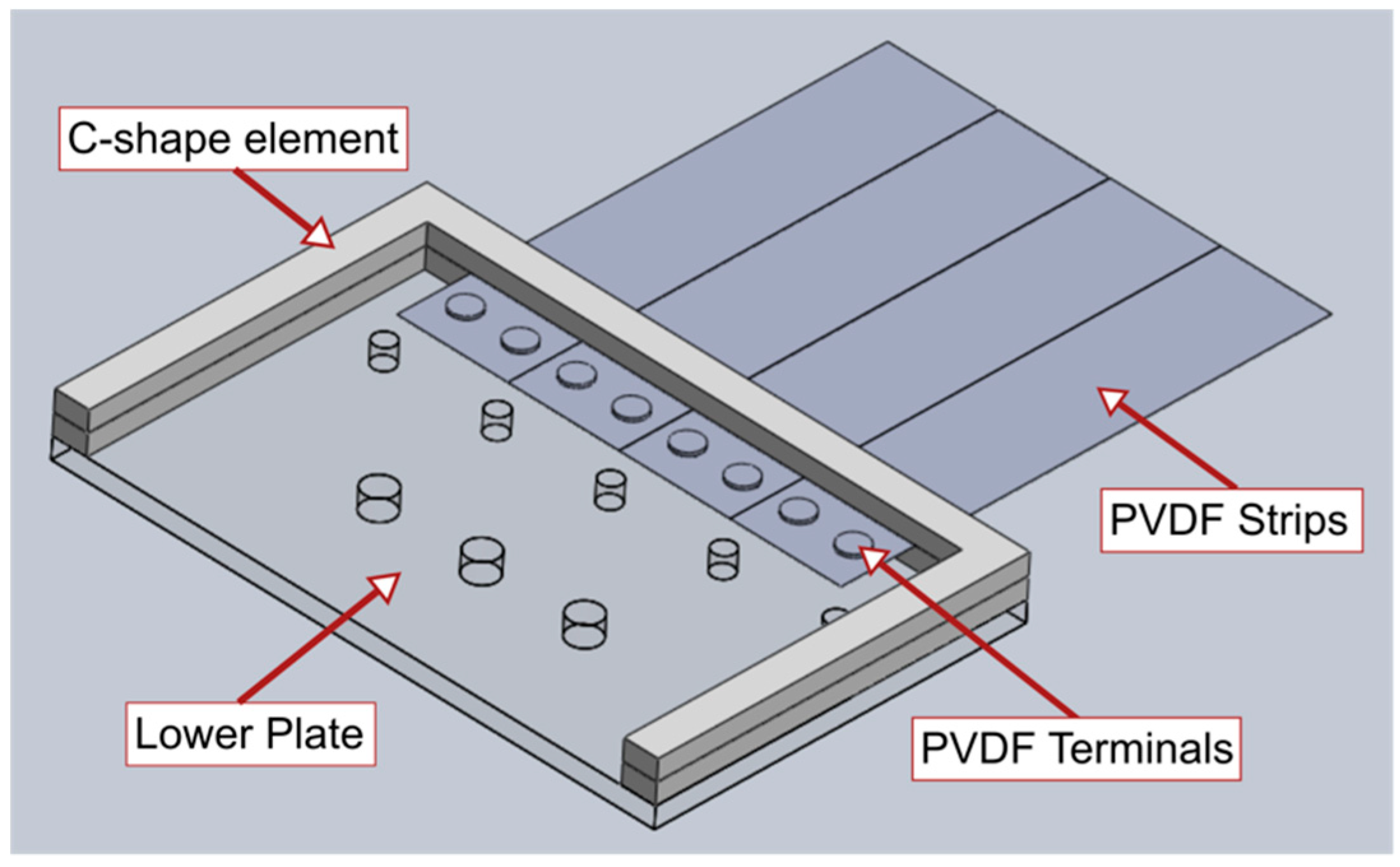
2.1. Piezo-Solar Inverted Flag Harvester

The piezo-solar inverted flag was realized with four PVDF elements (TE Connectivity Ltd, Schaffhausen, Switzerland (www.te.com); model LDT2-028K/L; length/width/thickness: 73/16/0.205 mm; density: 1780 kg/m³; Young modulus: 3 GPa; Poisson ratio: 0.34 [33]) and two flexible solar panels (Powerfilm Solar Inc., Ames, IA, USA (www.powerfilmsolar.com); model SP3-37; length/width/thickness: 36.5/64/0.2 mm; mass: 0.7 g), one attached at each side of the flag as shown in Figure 1d.

As can be noted in Figure 1d, the flexible solar panels are located close to the upstream leading edge of the inverted flag, such that their inclusion does not constrain the deformation of the flexible piezoelectric PVDF strips close to the fixed trailing edge of the flag where most of the mechanical strain is concentrated. It is evident that, in the present inverted flag design, the structural support is provided by the PVDF elements, while the solar panels constitute added masses. As is well known, tip masses can have huge influence on the dynamics of cantilevers, such that the inclusion of the solar panels onto the inverted flag can be expected to significantly affect the flag dynamics. In order to study this effect systematically, we realized two more inverted flags: one flag without solar panels and another with smaller solar panels, as shown in Figure 1b,c. As schematically indicated in Figure 1a, the configuration of the inverted flag can be characterized with three geometrical variables: (1) the overhang length L_p of the flag from the fixed support to the free tip; (2) the flag aspect ratio AR = L_p /W_p (ratio of flag length to flag width); and (3) the flag coverage ratio CR = L_s/L_p (ratio of solar panel length to flag length). The coverage ratio values for the three flags in Figure 1 were 0 (Figure 1b, referred to as no-solar flag), 0.32 (Figure 1c, referred to as half-solar flag), and 0.64 (Figure 1d, referred to as full-solar flag), while the overhang length L_p (57 mm) and aspect ratio AR (0.9) were not varied.

2.2. Experimental Set-Up and Methodology

The experimental set-up used to characterize the dynamics and power generation of the inverted flags is schematically shown in Figure 2. The downstream edge of the flags was connected with a purpose-built fixation clamp (see Figure 1b–d) to a vertical pole, which was placed in the middle of a wind tunnel (Armfield Limited, Ringwood, UK (armfieldonline.com)) with octagonal cross-section and height/width of 350 mm. The fixation clamp was manufactured from laser cut Perspex (Hobarts Laser Supplies, Leybourne, UK (https://hobarts.com); model: AC.CLR0000.03.3020) and was designed to hold the flag in a sandwich arrangement, realizing a cantilever boundary condition at the fixed edge of the flags. Construction details for the fixation clamp are provided in Appendix A.

Two light-emitting diode (LED) lights (Vibesta B.V., Helmond, The Netherland (www.vibesta.com); model: Capra 12 Daylight) were located on both sides of the wind tunnel and oriented perpendicularly to the rest position of the flag. The light intensity the flags were exposed to while at rest was measured with a portable light meter at 1.8 klx, and was not changed during the tests. Daylight intensity varies from about 10² lx at sunset/sundown to about 10⁵ lx in bright sunlight, with mid-range light intensities of 1–2 klx corresponding to a typical overcast day. The present results for solar power generation, therefore, can be regarded as indicative of the solar energy harvesting potential of the proposed flag harvester during an overcast day.

Prior to the tests, the flow in the wind tunnel was characterized with a calibrated single-probe hot-wire anemometer (Dantec Dynamics, Bristol, UK (www.dantecdynamics.com); probe type 55P15; 5-μm-diameter tungsten wire of 2 mm length operated in constant temperature mode). The boundary layer extended less than 5 mm from the walls of the wind tunnel at the lowest wind speed setting employed (1.5 m/s), and the velocity profile across the wind tunnel (excluding the boundary layer) was uniform to within 1%, i.e., velocity variations were on the order of the measuring error of the hot-wire probe. This assures that the inverted flags were always exposed to a fully developed velocity profile during the tests.

As shown in Figure 3, the streamwise turbulence intensity measured in the wind tunnel flow was around 0.5–0.8% within the range of free stream flow velocities from 4 m/s to 10 m/s of interest here, corresponding to mild turbulence. During the tests with the inverted flags, the wind speed in the wind tunnel was deduced (error within ±5%) from static/dynamic pressure measurements, using a calibrated pressure transducer (Sensirion AG, Staefa, Switzerland (www.sensirion.com); model: SDP816) connected to the wind tunnel with four static pressure ports located upstream of the inverted flag. Ambient temperature and pressure during the tests were 293 ± 1 K and 101 ± 1 kPa.

The motion of the flag was recorded with a digital camera (Panasonic Co., Osaka, Japan (www.panasonic.com); model: LUMIX DMC-FZ200; recording frequency: 200 fps; resolution: 480 × 640 pixels) located on top of the wind tunnel. In order to facilitate the optical tracking, a thin red paper tape was added to the upper border of the flags, as can be noted in Figure 1. The videos were post-processed with the Image Processing Toolbox of MATLAB (version R2015a), employing a tracking methodology previously used for flow-induced vibration and flexible fluid–structure interaction studies [34,35,36]. The motion of the flag was characterized with the instantaneous angular position $\theta \left(t\right)$ (measured to within ±2–3°), which is the angle between the tip of the flag at time $t$ and the flag rest position; and with the angular span of motion, which is the angle described between the two extreme positions spanned by the flag when observed from the top (see insert in Figure 4a). Locally, the flag possesses a variable curvature when deflected, such that the instantaneous angular position and the angular span of motion used here give a simple representative measure of the displacement for the whole flag. The power spectral density (PSD) was obtained by applying a fast Fourier transform (FFT) to the time series of the instantaneous angular position (using MATLAB built-in functions), and the frequency of flag flapping was identified as the dominant frequency (when present) in the power spectral density (uncertainty within 0.2–0.3 Hz, estimated from the full width at half maximum of the dominant peak in the power spectrum).

In addition, we reconstructed the trajectory of the system in phase-space (i.e., the system attractor) using the delayed vector method proposed by Bradley and Kantz [37]: a methodology developed for nonlinear time-series analysis that is particularly useful for fluid–structure interaction problems [34,35,36]. The topology of the reconstructed attractor of the inverted flag, in fact, gives a useful qualitative characterization of the flag dynamics, which completes and corroborates the quantitative information provided by the angular position and flapping frequency. The concept of phase-space representation, rather than a classic analysis in time or frequency domain, is the key point in nonlinear time-series analysis. The topology of the trajectory in phase-space of a nonlinear system, in fact, provides important qualitative information regarding the fundamental dynamics of the systems being investigated. The problem is that, in experimental studies, one normally observes a time series of scalar measurements of some quantity that depends on the current state of the system, and not the trajectory of the system in phase-space. The delayed vectors method [37] allows reconstructing the trajectory of the system in phase-space from a time series of scalar measurements, and can, therefore, be used in experimental studies such as the present one where only time series of scalar measurements of some quantity (the instantaneous angular position in the present case) are available. In the present case, the trajectory in phase-space was reconstructed by plotting the time-delayed instantaneous angular position $\theta \left(t+\tau \right)$ versus $\theta \left(t\right)$. If the delay $\tau$ is chosen properly (on the order of 40–60 ms in the present case), then the topology of the reconstructed attractor is representative of the underlying system dynamics [37].

The power generated by the inverted flag harvesters was collected and processed through LabVIEW 2017, while the data were gathered with a National Instruments (Austin, TX, USA (www.ni.com)) NI-USB-6225 external DAQ device. Following common practice in energy-harvesting studies, optimal load resistances that allowed peak power generation were empirically identified and employed. In order to collect the data from the individual solar panels and PVDF elements, separate circuits were built using prototyping breadboards that allowed circuit changes to be made quickly. The data acquisition program was written as a VI (Virtual Instrument) in LabVIEW 2017 using the standard DAQ-mx library. This program gathered, saved, and displayed the data in real time to allow an immediate impression of the power generated to be seen and to allow the load resistance to be set to give the highest power output. The sampling rate was set at 1 kHz to allow sufficient resolution of data through a flapping cycle for any particular flapping characteristics to be seen.

2.3. Numerical Model

Numerical simulations of the inverted flag dynamics were conducted by adopting a partitioned approach whereby the fluid dynamics and the structural dynamics are handled via their own separate field solvers, a rather common approach for fluid–structure interaction problems characterized by large structural displacements. The lattice-Boltzmann method [38], an alternative to traditional Navier–Stokes-based computational fluid dynamics solvers, was employed to solve the fluid dynamics. The governing equation for the lattice-Boltzmann method is the Boltzmann transport equation, given in discrete form by

$$f_i\left(\mathit{x}+{\mathit{c}}_i\Delta t,t+\Delta t\right)-f_i\left(\mathit{x},t\right)=\frac{\Delta t}{\tau }\left[f_i^{eq}\left(\mathit{x},t\right)-f_i\left(\mathit{x},t\right)\right]+\Delta t{F}_i\left(\mathit{x},t\right),$$

(1)

where $\mathit{x}$ represents the spatial coordinates, $t$ is time, ${\mathit{c}}_i$ is the $i$th component of the lattice velocity vector, and $F_i\left(\mathit{x},t\right)$ is a term accounting for the presence of an external force $f\left(\mathit{x},t\right)$ (e.g., gravity) [39]. The probability distribution function $f_i\left(\mathit{x},t\right)$ describes the proportion of fluid molecules within an elemental volume located at $\mathit{x}$ and time $t$ moving with velocity ${\mathit{c}}_i$. Equation (1) clearly shows a relaxation toward a local equilibrium. The equilibrium function $f_i^{eq}\left(\mathit{x},t\right)$ is obtained via a Taylor series [40] or Hermite polynomial [41] expansion of the Maxwell–Boltzmann distribution function and the relaxation time scale $\tau$ is directly related to the fluid viscosity [38]. Finally, the macroscopic fluid quantities can be recovered by taking moments of the probability function as follows:

$$\rho \left(\mathit{x},t\right)={\displaystyle \sum }_i{f}_i\left(\mathit{x},t\right),$$

(2)

$$\rho \mathit{v}\left(x,t\right)={\displaystyle \sum }_i{\mathit{c}}_i{f}_i\left(\mathit{x},t\right)+\frac{\Delta t}{2}f\left(\mathit{x},t\right).$$

(3)

The main advantage of the lattice-Boltzmann method is its amenability to parallel implementation, as well as the regular square lattice that aids with the solver coupling. Although not critical for the single-flag problem analyzed here, the parallel implementation capability will be instrumental in future studies to analyze the interaction among several flags. In fact, we envision that, in a real application, a harvester could combine several inverted flags properly tuned (via optimization of their geometry and/or mechanical properties) to yield the desired performance over the whole range of wind speeds and light conditions of interest for that particular application. The computational burden associated with analyzing and optimizing a multi-flag configuration will necessarily require a parallel implementation for time-efficient computation.

A co-rotational finite element method was adopted to solve the structural dynamics. Since large deformations are expected in the present work, a nonlinear Newton–Raphson solver was utilized. The governing equations for the system are given by [42]

$$\mathit{M}{\ddot{\mathit{U}}}^{n+1,k}+{\mathit{K}}^{n+1,k}\Delta {\mathit{U}}^k={\mathit{F}}_{ext}^{n+1}-{\mathit{F}}_{int}^{n+1,k},$$

(4)

$${\mathit{U}}^{n+1,k+1}={\mathit{U}}^{n+1,k}+\Delta {\mathit{U}}^k,$$

(5)

where $n$ and $k$ are the time step and iteration counters, $\mathit{M}$ is the mass matrix, $\mathit{K}$ is the tangent stiffness matrix, ${\mathit{F}}_{ext}$ is the external load vector (including fluid forces), ${\mathit{F}}_{int}$ represents the internal forces within the structure due to the stresses, $\ddot{\mathit{U}}$ represents the nodal accelerations, and $\Delta \mathit{U}$ represents the incremental nodal displacements. The system is iterated over until the incremental nodal displacements are sufficiently small, after which the solution is advanced to the next time step [43]. Second-order time integration is achieved via the implicit Newmark scheme. Since the inverted flag deformation is mainly two-dimensional (2D), 2D simulations were deemed appropriate. In particular, Euler–Bernoulli beam elements were used to model the flags, which is appropriate for structures with large length-to-thickness ratios such as the inverted flags of interest here.

The immersed boundary method [44] was used to couple the separate fluid dynamics and structural dynamics field solvers. This approach allows the fluid and structure to be solved on their own separate grids, and facilitates the transfer of information between them, thus simplifying the meshing and helping in capturing large deformations of the structure. However, specialized interpolation/spreading operators are required to transfer information between the two grids. Using lowercase notation for quantities on the fluid grid (Eulerian frame) and uppercase for the boundary grid (Lagrangian frame), these operators are given by

$$\Phi \left(\mathit{X}\right)=\mathcal{I}\left[\phi \left(\mathit{x}\right)\right]={\displaystyle \sum }_{{\Omega }_s}\phi \left(\mathit{x}\right)\tilde{\delta }\left(\mathit{x}-\mathit{X}\right)\Delta x\Delta y\Delta z,$$

(6)

$$\phi \left(\mathit{x}\right)=\mathcal{S}\left[\Phi \left(\mathit{X}\right)\right]={\displaystyle \sum }_{{\Gamma }_s}\Phi \left(\mathit{X}\right)\tilde{\delta }\left(\mathit{x}-\mathit{X}\right)\epsilon \Delta q\Delta r\Delta s,$$

(7)

where $\mathit{x}=\left(x,y,z\right)$, $\mathit{X}=\left(q,r,s\right)$, $\phi$ is a quantity defined on the fluid grid, $\Phi$ is the same quantity defined on the structure grid, $\tilde{\delta }$ is the discrete form of the Dirac delta function, and $ϵ$ is a scaling factor which ensures reciprocity between the interpolation and spreading steps [45]. Note that, for the regular Cartesian grid used here, $\Delta x=\Delta y=\Delta z=1$ in lattice units. Furthermore, for the one-dimensional (1D) line boundary used in this work, $\Delta q=\Delta r=1$. The spacing between immersed boundary points was chosen to match the lattice spacing such that $\Delta s=\Delta x=1$.

The coupled lattice-Boltzmann immersed boundary algorithm decomposes the velocity into a predicted and a force-corrected term [46]. Firstly, the lattice-Boltzmann step is computed without the immersed boundary to obtain a predicted velocity field ${\mathit{v}}^{*}$. From Equation (3), the corrected fluid velocity is, thus, given by

$$\rho \mathit{v}\left(\mathit{x},t\right)=\rho {\mathit{v}}^{*}\left(\mathit{x},t\right)+\frac{\Delta t}{2}\mathit{f}\left(\mathit{x},t\right).$$

(8)

Using the interpolation operator to convert this to the Lagrangian frame gives

$$\mathcal{I}\left[\rho \left(\mathit{x},t\right)\right]\mathit{V}\left(\mathit{X},t\right)=\mathcal{I}\left[\rho {\mathit{v}}^{*}\left(\mathit{x},t\right)\right]+\frac{\Delta t}{2}\mathit{F}\left(\mathit{X},t\right).$$

(9)

Since the velocity of the boundary $\mathit{V}\left(\mathit{X},t\right)=\mathcal{I}\left[\mathit{v}\left(\mathit{x},t\right)\right]$ is known, Equation (9) can be rearranged to solve for the corrective force term $\mathit{F}\left(\mathit{X},t\right)$. The corrective force is converted back to the Eulerian frame using the spreading operator and finally the velocity field is updated by adding the corrective force to the predicted velocity field via Equation (8). With regard to the structural calculation, $\mathit{F}\left(\mathit{X},t\right)$ is passed to the finite element method (FEM) solver such that ${\mathit{F}}_{ext}=\mathit{F}\left(\mathit{X},t\right)$ in the absence of any additional external forcing (e.g., gravity).

To ensure stability, a block Gauss–Seidel coupling scheme was adopted [47], whereby the field solvers are iterated over, within the current time step, until the interface conditions are satisfied. To accelerate the convergence of these iterations, a dynamic relaxation factor was used to relax the displacement of the structure after each iteration [47]. The resulting strongly coupled fluid–structure interaction numerical model is capable of handling the large nonlinear interactions associated with the inverted flag configuration. For more details regarding the model, the reader is directed to previous work [48].

To promote the onset of any instability, the flag was initialized with a small transverse displacement (1% of its length), i.e., the simulated flag at rest was slightly deflected on one side. After the initial transient, the simulations were run for approximately 20 flapping periods. The variation in thickness across the flag, associated with the presence of the solar panel, was properly accounted for in the structural solver. However, the immersed boundary, which is the geometry that the fluid “sees”, was represented as a line. This means that the variation in thickness across the flag due to the solar panel was not accounted for in the fluid solver. Although critical for the mechanical response of the flag, the variation in thickness across the flag was small enough to neglect its effect on the resulting flow field. For the scope of the present study, this was considered an acceptable approximation. Being located downstream of the flag, the support clamp that holds the flag in the wind tunnel does not significantly affect the flow development around the flag. Therefore, the support clamp was not modeled in the simulations, although the fixed edge of the flag was subjected to a local cantilever-type boundary condition that properly accounted for the support clamp.

The numerical simulations were set up to match the experimental conditions. However, to reduce the simulation run-time, the fluid viscosity was increased by three orders of magnitude, thus decreasing the Reynolds number proportionally. This follows the rationale successfully proposed for simulating flexible filaments [49] and inverted flags [50], and is here extended to composite inverted flags realized with flexible PVDF elements and flexible solar panels. In fluid–structure interaction problems characterized by large displacements, such as flexible filaments and the inverted flags of interest here, pressure forces control the interaction between the flow and the structure, whilst viscous effects play a comparatively minor role. This explains why numerical models simplified by artificially increasing the fluid viscosity can still capture the dynamics with reasonable accuracy [49,50], while achieving a much faster execution. Although not critical for the single-flag problem analyzed here, a fast execution will be instrumental in future studies to analyze the interaction among several flags and tailor the inverted flag harvesters to the intended final application. It is worth noting that more complex collision operators [51] could potentially allow stable solutions at higher Reynolds numbers. However, in light of the above discussion, this was deemed unnecessary for the present work. The regularized boundary condition [52] was used to impose the velocity at the inlet and far field boundaries, and a convective condition was imposed at the outlet [53]. Preliminary testing showed that a relaxation time scale of $\tau =0.57$ was sufficient to ensure a stable solution while, at the same time, limiting the lattice velocity to reduce compressibility effects. At the highest tested flow speed (12 m/s), the lattice velocity was found to be $v=0.035$, which results in a Mach number of $Ma=0.061$. This is well within the weakly compressible regime such that errors due to compressibility effects are limited.

All calculations were performed on a custom-built computer with a 3-GHz Intel Core i7-5960X processor (eight cores and two threads/core), and with 64 GB of random access memory (RAM).

3. Results and Discussion

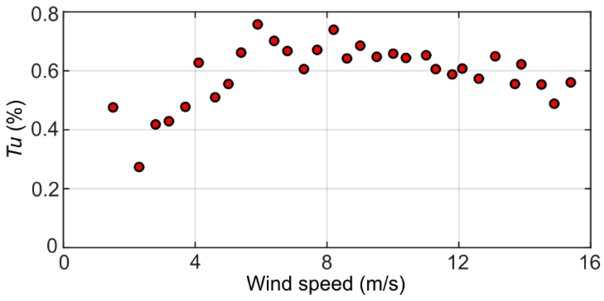
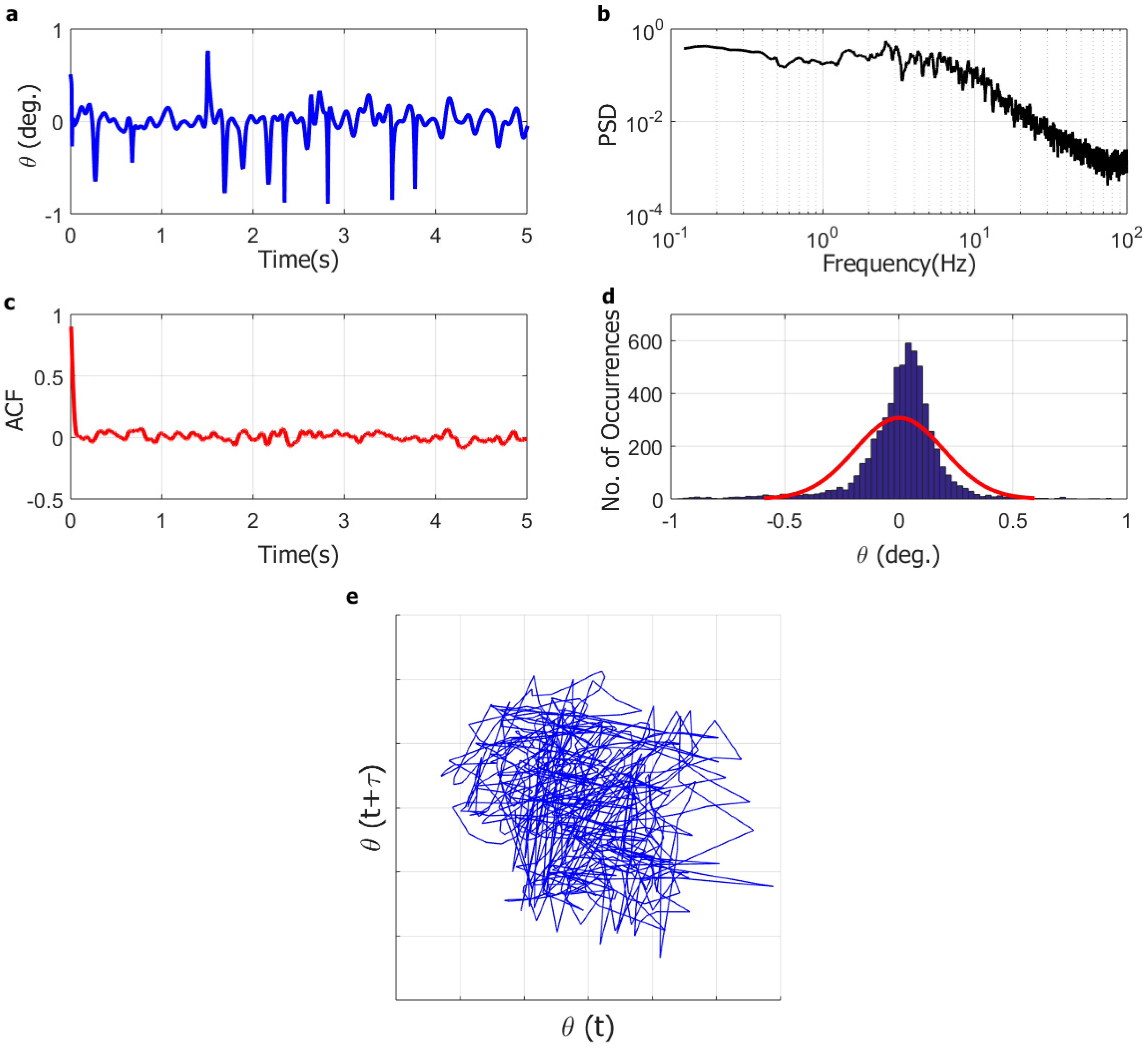
3.1. Inverted Flag Dynamics

The angular span of motion and the frequency of oscillation of the inverted flags, measured while gradually and stepwise increasing the wind speed from 0 m/s (no flow) to a maximum of about 10 m/s, are displayed in Figure 4. In particular, the absence of a dominant frequency of motion is indicated in Figure 4b with a null value of the frequency.

As can be noted in Figure 4, at low wind speed (below about 4–5 m/s), the angular span of motion and oscillating frequency are both zero, indicating that the inverted flags maintain their rest equilibrium configuration aligned with the incoming flow. As soon as the wind speed is large enough, the rest configuration becomes unstable and the flags start oscillating. During these oscillations, the angular span of motion gradually increases, as the wind speed is gradually increased, reaching a maximum of about 190° at a wind speed of 9 m/s. The frequency of oscillation, on the other hand, gradually decreases as the wind speed is gradually increased, although its variation is rather limited. The large-amplitude flapping oscillation persists until the wind speed is large enough to deflect the flag onto one side; in Figure 4, this corresponds to a wind velocity of about 10 m/s where the angular span of motion and the oscillating frequency are both zero.

The dynamic response of the full-solar flag at selected wind velocities is further analyzed in Figure 5, Figure 6 and Figure 7, which include (for the three representative wind speeds of 4.7 m/s, 9.0 m/s, and 9.7 m/s) (a) the instantaneous angular position time series (5-s sample); (b) the instantaneous angular position power spectral density (PSD); (c) the instantaneous angular position autocorrelation function; (d) the instantaneous angular position histogram (5-s sample; to help visualize the trend in the data, the histogram includes a red line corresponding to a normal density function fitted to the data); and (e) the reconstructed attractor in phase-space. As can be seen in Figure 5, at low wind speed (4.7 m/s), the flag is aligned with the incoming flow but appears to be not completely static. Rather, it undergoes small-amplitude oscillations (±1°) with no discernible dominant frequency, with a very fast-decaying autocorrelation function, with a bell-shaped histogram, and with a reconstructed attractor that covers the whole space.

At low wind speed, therefore, the flag dynamics appears to be a small-amplitude random vibration around the rest equilibrium configuration. The instantaneous angular position, however, is comparable in magnitude with the measuring error, such that the flag could also be actually static, and the measured motion could be the consequence of random noise pick-up from the instrumentation. The numerical simulations (described later) suggest that the flag is actually static, although, due to the limitations of the numerical model previously discussed, the possibility of a small random vibration cannot be ruled out. It is worth highlighting that the optical tracking system and the numerical model were conceived to capture the large flag displacements during flapping; thus, a relatively poor resolution of very small displacements is, to some extent, unavoidable and has no consequence on the conclusions of the present study.

At higher wind speed (9.0 m/s) in Figure 6, on the other hand, the instantaneous angular position time series is periodic and its power spectral density includes one dominant frequency with a few harmonics, the autocorrelation function is periodic and slowly decaying, the histogram is bridge-shaped, and the reconstructed attractor has a ring-like topology. This indicates that the flag dynamics at this wind speed involves a large-amplitude limit-cycle flapping oscillation.

Finally, at the highest wind speed tested (9.7 m/s) in Figure 7, the flag dynamics is qualitatively similar to what observed at low wind speed (4.7 m/s) in Figure 5; the flag apparently undergoes small-amplitude oscillations (±2–3°) with no discernible dominant frequency, the autocorrelation function decays fast, the histogram is bell-shaped, and the reconstructed attractor covers the whole space. Therefore, when the flag is fully deflected onto one side at very high wind speed, its dynamics appears to be a small-amplitude random vibration around the deflected configuration. Similarly to that previously discussed for the low wind speed of 4.7 m/s, the instantaneous angular position is comparable in magnitude with the measuring error; thus, the small-amplitude vibration cannot be duly resolved with the present set-up. As previously noted, this limitation has no consequence on the conclusions of the present study.

The dynamics analysis carried out for the no-solar and the half-solar flags yielded results qualitatively analogous to those obtained for the full-solar flag presented in Figure 5, Figure 6 and Figure 7. For the sake of brevity, these are not documented here. In conclusion, all three main dynamic responses of inverted flags identified in previous research and previously discussed (i.e., static-aligned, flapping, and fully deflected) are, therefore, clearly observable in the present results, and this qualitatively validates the present approach.

As evident in Figure 4, the inclusion of the solar panels has a destabilizing effect on the dynamics of the inverted flag. The added mass of the solar panels, in fact, reduces the wind speed required to trigger the large-amplitude limit-cycle oscillation, widens the wind speed window where limit-cycle oscillations are sustained, and increases the angular span of motion at any given wind speed. These observations are consistent with the expected destabilizing effect of the solar panels that constitute a tip added mass onto the inverted flag, which can be regarded as a cantilever. The frequency of oscillation decreases when adding the solar panels, consistently indicating that a heavier flag flaps at a lower frequency with respect to a lighter one. The transition from the large-amplitude flapping to the small-amplitude vibration around the fully deflected configuration, however, is not significantly affected by the inclusion of the solar panels. It is evident from the results presented that the dynamics of the inverted flags remains qualitatively the same when the solar panels are included, because all three main dynamics modes of inverted flags (static-aligned, flapping, and fully deflected) are still observable. Importantly, the inclusion of the solar panels widens the wind speed window where limit-cycle oscillations are sustained, which is the mode of operation of interest for energy harvesting with PVDF elements.

Noteworthy, the inverted flags exhibited a rather pronounced hysteresis in their dynamics, as illustrated for the full-solar flag in Figure 8, where the angular span of motion is plotted for increasing and then decreasing wind speed. As can be noted, once the wind speed gradually increased to a value large enough to fully deflect the flag, then the wind velocity was reduced considerably before the large-amplitude limit-cycle flapping resumed. This hysteresis can be traced back to the mechanical properties of the PVDF elements that make up the flags. In particular, the high flexibility of the PVDF elements comes at the expense of a limited elasticity, which prevents the flags from resuming the flapping motion once they reach the fully deflected configuration at high wind speed, unless the wind speed is reduced substantially.

The hysteresis in the inverted flag response, clearly not ideal for final applications, will be alleviated in future optimization studies using custom-made PVDF elements with mechanical properties tailored to the intended application, instead of the off-the-shelf PVDF elements used here. A different approach to alleviate the inverted flag hysteresis was explored by Silva-Leon et al. [54], who included a metal shim in their inverted flags. In their design, the structural support to the flag was provided by the metal shim, whilst the PVDF elements and the solar panels were added masses attached onto the metal shim. The higher elasticity of the metal shim helped in reducing the hysteresis, although it also made their flags more rigid and, therefore, more stable, such that the wind speed required to sustain large-amplitude flapping increased substantially.

3.2. Numerical Simulations

The comparison between measurements and numerical predictions is provided in Figure 9a,b, where the predicted angular span of motion and frequency of oscillation are compared with the corresponding measurements for the no-solar and the full-solar flags. Overall, the agreement between measurements and predictions is encouraging. This indicates that, despite the simplifications previously discussed, the present numerical modeling approach is capable of reproducing the inverted flag dynamics. In particular, the location and extent of the flapping is predicted reasonably well by the numerical model, and the predicted values of the angular span of motion and frequency of oscillation compare well with the measurements. However, there is a noticeable difference for the no-solar flag that is predicted to flap at lower wind speeds with respect to the measurements. This can be explained by three-dimensional (3D) effects in the deformation of the flags, which were shown to increase stability in the conventional flag configuration [55] but are not captured by the present 2D numerical model. Interestingly, the agreement between predictions and measurements is better for the full-solar flag, even though the wind velocity for the onset of flapping is slightly over predicted. As better discussed in the next paragraph, this indicates that the stiffening of the flag due to the inclusion of the solar panels may reduce 3D effects, as compared with the no-solar flag, thus yielding a better agreement between measurements and 2D simulations.

It is important to note that the assumption of high aspect ratio implicit in a 2D simulation is expected to have an impact on the point of onset of flapping, where it was shown that, as the aspect ratio reduces, the velocity required to initiate flapping is increased. Aspect ratio effects are beyond the scope of the present work; instead, the reader is directed to the works of Sader et al. [56] and Tavallaeinejad et al. [57] for further details.

Predicted envelopes of motion for the no-solar and the full-solar flags are provided in Figure 9c, while accompanying videos are included as Supplementary Materials. Whilst the critical flow velocity for each state is different between the two cases, both exhibit a transition from a static zero-deflection state, through small-amplitude and large-amplitude flapping states, and finally a large-deflection static state. More importantly, in the full-solar case, the bending deformation is localized toward the root of the flag, with very little bending toward the tip due to the stiffening effect of the solar panels. As previously noted, this stiffening reduces 3D effects in the deformation of the flag, which is a beneficial outcome with respect to the applicability of 2D numerical simulations. On the other hand, the stiffening of the flag reduces the local deformation of the PVDF elements, thus reducing the mechanical strain and, therefore, the piezoelectric power generation, even though the additional power generation from the solar panels compensates for this (this is quantitatively assessed in Section 3.3 later on). Therefore, in the present inverted flag design, the solar panels are not only a destabilizing added mass; they also affect the local rigidity of the flag along its length, possibly reducing 3D effects.

Finally, the results of a sensitivity study carried out with the present numerical model for the full-solar flag are presented in Figure 10, where the predicted angular span and frequency of oscillation are displayed as functions of the wind speed for (a) varying flag length L_p, (b) varying Young’s modulus E (hence, stiffness of the flag), and (c) varying coverage ratio (CR). It is evident that the flag length and the Young’s modulus have a significant impact on the dynamics of the flag, whilst the coverage ratio has a comparatively lower influence. In particular, shorter/longer flags flap at higher/lower wind velocities with higher/lower frequencies, consistently indicating that a longer cantilever is more prone to instability and, being heavier, flaps at a lower frequency with respect to a shorter and lighter one. Furthermore, increasing the Young’s modulus makes the flag more rigid, thus increasing the wind velocity required to sustain flapping and the corresponding flapping frequency. This confirms that, as noted previously, having the PVDF elements custom-made to the desired mechanical properties will be a viable strategy to tailor the inverted flag harvester to the intended application, and the present numerical model would be instrumental in informing the harvester optimization.

The run-time of each simulation included in Figure 10 was on the order of 10 h (single thread): fast enough to allow time-efficient exploration of the (highly dimensional) parameter space of inverted flags. In addition to informing the future optimization of the harvester, the numerical tool will also be instrumental in informing future experiments on the fundamental coupled dynamics of multiple flag arrangements. In fact, having a preliminary indication on the dynamics of a multi-flag arrangement, for given flag geometry and constitutive material properties, would provide guidance on how to actually realize the flags, and would also inform the design of the experimental apparatus to track the flag dynamics and measure the flow field.

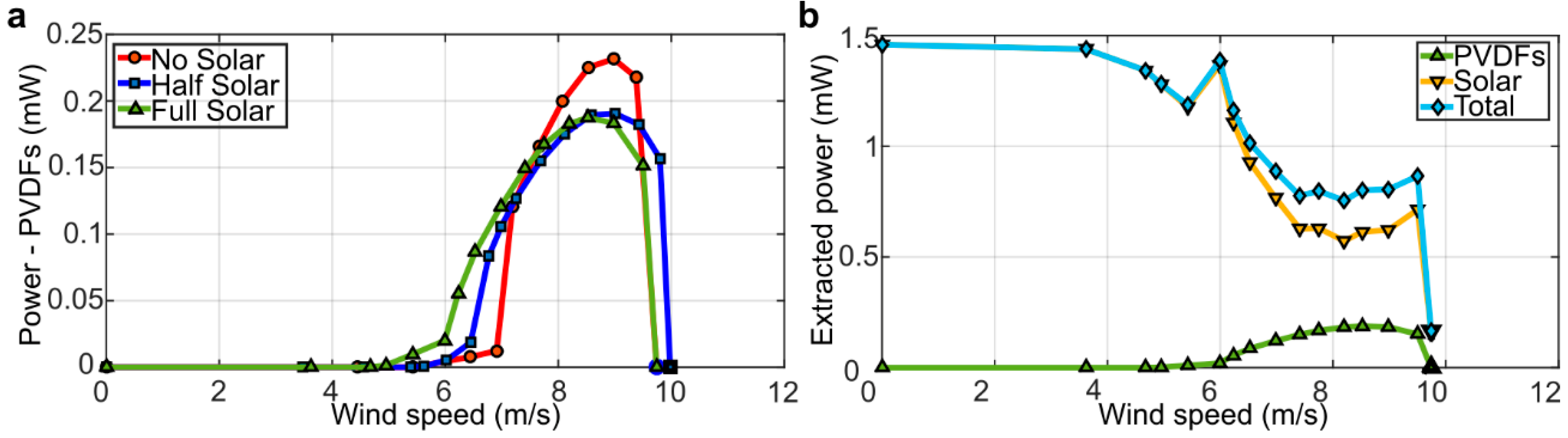
3.3. Power Generation

The piezoelectric power, calculated from the root-mean-square (RMS) value of the measured voltage generated by the inverted flags for increasing wind speed, is provided in Figure 11a. As can be noted, up to a wind speed of about 7.5 m/s, the piezoelectric power generation is congruent with the angular span of motion in Figure 4a, consistently indicating that a larger angular span of motion yields a larger strain and, therefore, a larger power generation from the PVDF elements. This is no longer the case, however, at wind speeds above about 7.5 m/s, when the half-solar and the full-solar flags follow similar trends, while the no-solar flag yields more power. This confirms the simulation results previously discussed, indicating that the stiffening of the flag due to the inclusion of the solar panels reduces the local deformation of the PVDF elements, thus reducing the mechanical strain and, consequently, the piezoelectric power generation.

The piezoelectric, solar, and total power outputs generated by the full-solar flag for increasing wind speed are presented in Figure 11b. In particular, the solar power levels shown are the average values of power generated, while the total power is the sum of the piezoelectric and solar contributions. As can be noted in Figure 11b, the solar power output is higher when the flag is at rest, while it decreases during flapping. This is due to the lighting configuration adopted here, which is indicative in magnitude of an overcast day, although the lighting is more directional than what would be observed in a real ambient application. It is nonetheless evident in Figure 11b that the proposed piezo/solar inverted flag harvester is a promising concept, capable of harvesting kinetic wind energy and solar radiant energy at the same time and generating enough power (about 1 mW) to supply low-power electronic devices. In particular, the additional power generated by the solar panels more than compensates for the lower piezoelectric power output due to the stiffening of the flag from the inclusion of the solar panels. Perhaps even more importantly, the possibility to harvest wind and solar energies at the same time will accommodate for the inherent intermittency of these energy sources in real ambient applications. Wind and solar energies, in fact, have intermittencies that tend to mutually compensate, because the wind typically blows during stormy conditions when the sun does not shine, whilst, conversely, the sun typically shines on calm days with little wind.

To better assess the performance of the present inverted flag harvester,

Table 1. Power density comparison of different harvesters based on polyvinylidene fluoride (PVDF) elements.

Reference	PVDF Model	Power Density (mW/cm3)	Wind Speed (m/s)
Vatansever et al. [20]	LDT4-028K/L	0.16	10
Li et al. [24]	LDT2-028K/L	0.871	8
Hobeck and Inman [27]	LDT4-028K/L	0.0051	7
Present study: no-solar flag	LDT4-028K/L	0.27	8.5
Present study: full-solar flag	LDT4-028K/L	0.48	8.5

provides a comparison against other concepts available in the literature. Note that, for consistency, the comparison here is only limited to harvesters based on PVDF elements and tested in controlled wind conditions. Following common practice in energy harvesting, the power densities included in Table 1 were calculated based on the total volume of the harvesters. As can be noted, the power density of the present inverted flag harvester is rather good, and the inclusion of the solar panels almost doubles the power density. This is encouraging, particularly when considering that the present work was essentially a proof of concept, which motivates further study to improve and optimize the proposed harvester.

4. Conclusions

The flow-induced dynamics and power generation of an energy harvester based on the inverted flag design were investigated with experiments and numerical simulations. The energy harvester was realized using off-the-shelf flexible piezoelectric PVDF strips and flexible mini solar panels to simultaneously harvest wind kinetic energy and solar radiant energy, with a view at compensating the inherent intermittency of ambient energy sources. In the proposed design, the PVDF strips made up the flag harvester, thus providing the structural support, while the solar panels were incorporated as tip masses close to the flag free edge. The performance of the energy harvester was experimentally investigated under controlled wind (up to 10 m/s wind speed) and light exposure (1.8 klx), and simulations based on a lattice-Boltzmann/finite-element/immersed-boundary numerical method were used to corroborate and integrate the measurements. The measurements indicate that the proposed harvester is a promising concept, capable of producing enough power (on the order of 1 mW) to supply low-power electronic devices for distributed sensor networks. In addition to harvesting solar radiant energy, the solar panels make the inverted flag more rigid but also widen the wind speed window where limit-cycle oscillations are sustained, which is the mode of operation of interest for energy harvesting with PVDF elements. Notwithstanding key simplifications implemented to achieve a fast execution, the numerical model developed is capable of capturing the essential dynamics of the inverted flag harvester, and was instrumental in better assessing the role of the solar panels onto the flag dynamics. Sensitivity simulations highlighted the influence of the flag length and Young’s modulus on the dynamic response. A limitation of the proposed design is the hysteresis observed in the dynamics of the harvester when increasing and decreasing the wind flow speed. This is related to the limited elasticity of the PVDF elements that make up the harvester, and will be corrected in future studies using custom-made PVDF elements with optimized mechanical properties. The numerical model executes quickly and is amenable to parallel implementation, and it will be instrumental in future optimization studies for a time-effective exploration of the high-dimensional parameter space of inverted flag harvesters.

References

1. Paradiso, J.A.; Starner, T. Energy scavenging for mobile and wireless electronics. IEEE Pervasive Comput. 2005, 4, 18–27. [Google Scholar] [CrossRef]
2. Mathúna, C.Ó.; O’Donnell, T.; Martinez-Catala, R.V.; Rohan, J.; O’Flynn, B. Energy scavenging for long-term deployable wireless sensor networks. Talanta 2008, 75, 613–623. [Google Scholar] [CrossRef]
3. Hu, Y.; Zhang, Y.; Xu, C.; Lin, L.; Snyder, R.L.; Wang, Z.L. Self-powered system with wireless data transmission. Nano Lett. 2011, 11, 2572–2577. [Google Scholar] [CrossRef] [PubMed]
4. Wang, Z.L.; Zhu, G.; Yang, Y.; Wang, S.; Pan, C. Progress in nanogenerators for portable electronics. Mater. Today 2012, 15, 532–543. [Google Scholar] [CrossRef]
5. Gubbi, J.; Buyya, R.; Marusic, S.; Palaniswami, M. Internet of Things (IoT): A vision, architectural elements, and future directions. Future Gener. Comput. Syst. 2013, 29, 1645–1660. [Google Scholar] [CrossRef] [Green Version]
6. Hancke, G.P.; de Carvalho e Silva, B.; Hanche, G.P. The role of advanced sensing in Smart Cities. Sensors 2013, 13, 393–425. [Google Scholar] [CrossRef]
7. Erturk, A.; Inman, D.J. An experimentally validated bimorph cantilever model for piezoelectric energy harvesting from base excitations. Smart Mater. Struct. 2009, 18, 025009. [Google Scholar] [CrossRef]
8. Renno, J.M.; Daqaq, M.F.; Inman, D.J. On the optimal energy harvesting from a vibration source. J. Sound Vib. 2009, 320, 386–405. [Google Scholar] [CrossRef]
9. Stanton, S.C.; Erturk, A.; Mann, B.P.; Inman, D.J. Nonlinear piezoelectricity in electro-elastic energy harvesters: Modelling and experimental identification. J. Appl. Phys. 2010, 108, 074903. [Google Scholar] [CrossRef]
10. Abdelkefi, A.; Najar, F.; Nayfeh, A.H.; Ayed, S.B. An energy harvester using piezoelectric cantilever beams undergoing coupled bending–torsion vibrations. Smart Mater. Struct. 2011, 20, 115007. [Google Scholar] [CrossRef]
11. Doaré, O.; Michelin, S. Piezoelectric coupling in energy-harvesting fluttering flexible plates: Linear stability analysis and conversion efficiency. J. Fluids Struct. 2011, 27, 1357–1375. [Google Scholar] [CrossRef]
12. Michelin, S.; Doaré, O. Energy harvesting efficiency of piezoelectric flags in axial flows. J. Fluid Mech. 2013, 714, 489–504. [Google Scholar] [CrossRef] [Green Version]
13. Hobeck, J.D.; Inman, D.J. A distributed parameter electromechanical and statistical model for energy harvesting from turbulence-induced vibration. Smart Mater. Struct. 2014, 23, 115003. [Google Scholar] [CrossRef]
14. Nabawy, M.R.A.; Parslew, B.; Crowther, W.J. Dynamic performance of unimorph piezoelectric bending actuators. Proc. Inst. Mech. Eng. I J. Syst. Control Eng. 2015, 229, 118–129. [Google Scholar] [CrossRef]
15. McCarty, J.M.; Watkins, S.; Deivasigamani, A.; John, S.J. Fluttering energy harvesters in the wind: A review. J. Sound Vib. 2016, 361, 355–377. [Google Scholar] [CrossRef]
16. Nabavi, S.; Zhang, L. Portable wind energy harvesters for low-power applications: A survey. Sensors 2016, 16, 1101. [Google Scholar] [CrossRef] [PubMed]
17. Nabawy, M.R.A.; Crowther, W.J. Dynamic electromechanical coupling of piezoelectric bending actuators. Micromachines 2016, 7, 12. [Google Scholar] [CrossRef]
18. Shoele, K.; Mittal, R. Flutter instability of a thin flexible plate in a channel. J. Fluid Mech. 2016, 786, 29–46. [Google Scholar] [CrossRef]
19. Shoele, K.; Mittal, R. Energy harvesting by flow-induced flutter in a simple model of an inverted piezoelectric flag. J. Fluid Mech. 2016, 790, 582–606. [Google Scholar] [CrossRef]
20. Vatansever, D.; Hadimani, R.L.; Shah, T.; Siores, E. An investigation of energy harvesting from renewable sources with PVDF and PZT. Smart Mater. Struct. 2011, 20, 055019. [Google Scholar] [CrossRef]
21. Kim, D.; Cossé, J.; Huertas Cerdeira, C.; Gharib, M. Flapping dynamics of an inverted flag. J. Fluid Mech. 2013, 736, R1. [Google Scholar] [CrossRef]
22. Cossé, J.; Sader, J.; Kim, D.; Huertas Cerdeira, C.; Gharib, M. The effect of aspect ratio and angle of attack on the transition regions of the inverted flag instability. In Proceedings of the ASME 2014 Pressure Vessels & Piping Conference, Anaheim, CA, USA, 20–24 July 2014. PVP2014-28445. [Google Scholar]
23. Orrego, S.; Shoele, K.; Ruas, A.; Doran, K.; Caggiano, B.; Mittal, R.; Kang, S.H. Harvesting ambient wind energy with an inverted piezoelectric flag. Appl. Energy 2017, 194, 212–222. [Google Scholar] [CrossRef]
24. Li, S.; Yuan, J.; Lipson, H. Ambient wind energy harvesting using cross-flow fluttering. J. Appl. Phys. 2011, 109, 026104. [Google Scholar] [CrossRef]
25. McCarty, J.M.; Deivasigamani, A.; John, S.J.; Watkins, S.; Coman, F.; Petersen, P. Downstream flow structures of a fluttering piezoelectric energy harvester. Exp. Them. Fluid Sci. 2013, 51, 279–290. [Google Scholar] [CrossRef]
26. McCarty, J.M.; Deivasigamani, A.; Watkins, S.; John, S.J.; Coman, F.; Petersen, P. On the visualisation of flow structures downstream of fluttering piezoelectric energy harvesters in a tandem configuration. Exp. Them. Fluid Sci. 2014, 57, 407–419. [Google Scholar] [CrossRef]
27. Hobeck, J.D.; Inman, D.J. Artificial piezoelectric grass for energy harvesting from turbulence-induced vibration. Smart Mater. Struct. 2012, 21, 105024. [Google Scholar] [CrossRef]
28. Shi, S.; New, T.H.; Liu, Y. Flapping dynamics of a low aspect-ratio energy-harvesting membrane immersed in a square cylinder wake. Exp. Them. Fluid Sci. 2013, 46, 151–161. [Google Scholar] [CrossRef]
29. Shi, S.; New, T.H.; Liu, Y. Effects of aspect-ratio on the flapping behaviour of energy-harvesting membrane. Exp. Them. Fluid Sci. 2014, 52, 339–346. [Google Scholar] [CrossRef]
30. Erturk, A.; Delporte, G. Underwater thrust and power generation using flexible piezoelectric composites: An experimental investigation toward self-powered swimmer-sensor platforms. Smart Mater. Struct. 2011, 20, 125013. [Google Scholar] [CrossRef]
31. Haji, M.N.; Kluger, J.M.; Sapsis, T.P.; Slocum, A.H. A symbiotic approach to the design of offshore wind turbines with other energy harvesting systems. Ocean Eng. 2018, 169, 673–681. [Google Scholar] [CrossRef]
32. Iqbal, M.; Khan, F.U. Hybrid vibration and wind energy harvesting using combined piezoelectric and electromagnetic conversion for bridge health monitoring applications. Energy Convers. Manag. 2018, 172, 611–618. [Google Scholar] [CrossRef]
33. Deivasigamani, A.; McCarthy, J.M.; John, S.; Watkins, S.; Coman, F. Investigation of asymmetrical configurations for piezoelectric energy harvesting from fluid flow. In Proceedings of the ASME 2014 Conference on Smart Materials, Adaptive Structures and Intelligent Systems, New Port, RI, USA, 8–10 September 2014. [Google Scholar]
34. Cioncolini, A.; Silva-Leon, J.; Cooper, D.; Quinn, M.K.; Iacovides, H. Axial-flow-induced vibration experiments on cantilevered rods for nuclear reactor applications. Nucl. Eng. Des. 2018, 338, 102–118. [Google Scholar] [CrossRef]
35. Silva-Leon, J.; Cioncolini, A.; Filippone, A.; Domingos, M. Flow-induced motions of flexible filaments hanging in cross-flow. Exp. Therm. Fluid Sci. 2018, 97, 254–269. [Google Scholar] [CrossRef]
36. Silva-Leon, J.; Cioncolini, A. Modulation of flexible filament dynamics due to attachment angle relative to the flow. Exp. Therm. Fluid Sci. 2019, 102, 232–244. [Google Scholar] [CrossRef]
37. Bradley, E.; Kantz, H. Non-linear time-series analysis revisited. Chaos 2015, 25, 097610. [Google Scholar] [CrossRef] [PubMed]
38. Chen, S.; Doolen, G. Lattice Boltzmann method for fluid flows. Annu. Rev. Fluid Mech. 1998, 30, 329–364. [Google Scholar] [CrossRef]
39. Guo, Z.; Zheng, C.; Shi, B. Discrete lattice effects on the forcing term in the lattice Boltzmann method. Phys. Rev. E 2002, 65, 046308. [Google Scholar] [CrossRef]
40. He, X.; Luo, L. A priori derivation of the lattice Boltzmann equation. Phys. Rev. E 1997, 55, R6333. [Google Scholar] [CrossRef]
41. Shan, X.; He, X. Discretization of the velocity space in the solution of the Boltzmann equation. Phys. Rev. Lett. 1998, 80, 65–68. [Google Scholar] [CrossRef]
42. Bathe, K.J. Finite Element Procedures, 2nd ed.; Prentice Hall: Upper Saddle River, NJ, USA, 2014. [Google Scholar]
43. Zienkiewicz, O.J.; Taylor, R.L.; Fox, D. The Finite Element Method for Solid and Structural Mechanics, 7th ed.; Butterworth-Heinemann: Oxford, UK, 2014. [Google Scholar]
44. Mittal, R.; Iaccarino, G. Immersed boundary methods. Annu. Rev. Fluid Mech. 2005, 37, 239–261. [Google Scholar] [CrossRef]
45. Pinelli, A.; Naqavi, I.Z.; Piomelli, U.; Favier, J. Immersed-boundary methods for general finite-difference and finite-volume Navier-Stokes solvers. J. Comput. Phys. 2010, 229, 9073–9091. [Google Scholar] [CrossRef]
46. Li, Z.; Favier, J.; D’Ortona, U.; Poncet, S. An immersed boundary-lattice Boltzmann method for single- and multi-component fluid flows. J. Comput. Phys. 2016, 304, 424–440. [Google Scholar] [CrossRef] [Green Version]
47. Kuttler, U.; Wall, W.A. Fixed-point fluid-structure interaction solvers with dynamic relaxation. Comput. Mech. 2008, 43, 61–72. [Google Scholar] [CrossRef]
48. Harwood, A.R.G.; O’Connor, J.; Munoz, J.S.; Santasmasas, M.C.; Revell, A.J. LUMA: A many-core, fluid-structure interaction solver based on the lattice-Boltzmann method. SoftwareX 2018, 7, 88–94. [Google Scholar] [CrossRef]
49. Zhu, L.; Peskin, C. Simulation of a flapping flexible filament in a flowing soap film by the immersed boundary method. J. Comput. Phys. 2002, 179, 452–468. [Google Scholar] [CrossRef]
50. Ryu, J.; Park, S.; Kim, B.; Sung, H. Flapping dynamics of an inverted flag in a uniform flow. J. Fluids Struct. 2015, 57, 159–169. [Google Scholar] [CrossRef]
51. De Rosis, A.; Lévêque, E. Central-moment lattice Boltzmann schemes with fixed and moving immersed boundaries. Comput. Math. Appl. 2016, 72, 1616–1628. [Google Scholar] [CrossRef]
52. Latt, J.; Chopard, B.; Malaspinas, O.; Deville, M.; Michler, A. Straight velocity boundaries in the lattice Boltzmann method. Phys. Rev. E 2008, 77, 056703. [Google Scholar] [CrossRef] [PubMed]
53. Yang, Z. Lattice Boltzmann outflow treatments: Convective conditions and others. Comput. Math. Appl. 2013, 65, 160–171. [Google Scholar] [CrossRef]
54. Silva-Leon, J.; Cioncolini, A.; Nabawy, M.N.A.; Revell, A.; Kennaugh, A. Simultaneous wind and solar energy harvesting with inverted flags. Appl. Energy 2019, 239, 846–858. [Google Scholar] [CrossRef]
55. Eloy, C.; Souilliez, C.; Schouveiler, L. Flutter of a rectangular plate. J. Fluids Struct. 2007, 23, 904–919. [Google Scholar] [CrossRef] [Green Version]
56. Sader, J.E.; Huertas-Cerdeira, C.; Gharib, M. Stability of slender inverted flags and rods in uniform steady flow. J. Fluid Mech. 2016, 809, 873–894. [Google Scholar] [CrossRef]
57. Tavallaeinejad, M.; Païdoussis, M.P.; Legrand, M. Nonlinear static response of low-aspect-ratio inverted flags subjected to a steady flow. J. Fluid Struct. 2018, 83, 413–428. [Google Scholar] [CrossRef]
Figure 1. Configuration of the piezo-solar flags used in this study: a flag is made of four flexible polyvinylidene fluoride (PVDF) elements and two mini solar panels attached to both sides at the tip. (a) The dimensions used to describe the geometry of a flag; (b) no-solar flag (coverage ratio (CR) = 0); (c) half-solar flag (CR = 0.32); (d) full-solar flag (CR = 0.64) (the flow direction is left to right).
Fluids 04 00087 g001
Figure 2. Schematics of the experimental set-up used to characterize the dynamics and power generation of the flags subjected to controlled wind and light excitation.
Fluids 04 00087 g002
Figure 3. Streamwise turbulence intensity vs. wind speed.
Fluids 04 00087 g003
Figure 4. Experimental measurements of the dynamics of the inverted flags: (a) angular span of motion vs. wind speed; (b) dominant frequency of motion vs. wind speed.
Fluids 04 00087 g004
Figure 5. Representative dynamics of aligned-vibrating regime for the full-solar flag at wind speed of 4.7 m/s: (a) angular position time series (5 s); (b) angular position power spectral density (PSD); (c) angular position autocorrelation function (ACF); (d) angular position histogram; (e) system trajectory in phase-space (reconstructed attractor).
Fluids 04 00087 g005
Figure 6. Representative dynamics of flapping regime for the full-solar flag at wind speed of 9.0 m/s: (a) angular position time series (5 s); (b) angular position power spectral density (PSD); (c) angular position autocorrelation function (ACF); (d) angular position histogram; (e) system trajectory in phase-space (reconstructed attractor).
Fluids 04 00087 g006
Figure 7. Representative dynamics of deflected regime for the full-solar flag at wind speed of 9.7 m/s: (a) angular position time series (5 s); (b) angular position power spectral density (PSD); (c) angular position autocorrelation function (ACF); (d) angular position histogram; (e) system trajectory in phase-space (reconstructed attractor).
Fluids 04 00087 g007
Figure 8. Representative hysteresis cycle for the full-solar flag.
Fluids 04 00087 g008
Figure 9. Comparison of the numerical solver simulation results with experimental measurements: (a) no-solar flag; (b) full-solar flag. (i) Angular span of motion vs. wind speed; (ii) dominant frequency vs. wind speed; (c) envelopes of motion from the numerical simulations at various wind speeds.
Fluids 04 00087 g009
Figure 10. Sensitivity analysis on the dynamics of the full-solar flag. Effect of varying (a) the flag length, (b) the Young’s modulus, and (c) the coverage ratio. (i) Angular span of motion vs. wind speed; (ii) flapping frequency vs. wind speed.
Fluids 04 00087 g010
Figure 11. Measured power generation for the inverted flags: (a) root-mean-square (RMS) power generated from the four PVDF elements at different wind speeds; (b) total extracted power from the full-solar flag including the contributions from the four PVDF elements and the two full-solar panels (at 1.8 klx constant illumination).
Fluids 04 00087 g011