Article

Turbulence and Microprocesses in Inhomogeneous Solar Wind Plasmas

by
Catherine Krafft
1,*,
Alexander S. Volokitin
2,3 and
Gaëtan Gauthier
1
1
Laboratoire de Physique des Plasmas, Centre National de la Recherche Scientifique, Ecole Polytechnique, Sorbonne Université, Université Paris-Saclay, Observatoire de Paris, PSL Research University, 91128 Palaiseau, France
2
Space Research Institute, 84/32 Profsoyuznaya Str., 117997 Moscow, Russia
3
Pushkov Institute of Terrestrial Magnetism, Ionosphere and Radio Wave Propagation, Troitsk, 142190 Moscow, Russia
*
Author to whom correspondence should be addressed.
Fluids 2019, 4(2), 69; https://doi.org/10.3390/fluids4020069
Submission received: 9 February 2019 / Revised: 27 March 2019 / Accepted: 6 April 2019 / Published: 11 April 2019
(This article belongs to the Special Issue Modelling of Plasma Flow)

Abstract

:
The random density fluctuations observed in the solar wind plasma crucially influence on the Langmuir wave turbulence generated by energetic electron beams ejected during solar bursts. Those are powerful phenomena consisting of a chain of successive processes leading ultimately to strong electromagnetic emissions. The small-scale processes governing the interactions between the waves, the beams and the inhomogeneous plasmas need to be studied to explain such macroscopic phenomena. Moreover, the complexity induced by the plasma irregularities requires to find new approaches and modelling. Therefore theoretical and numerical tools were built to describe the Langmuir wave turbulence and the beam’s dynamics in inhomogeneous plasmas, in the form of a self-consistent Hamiltonian model including a fluid description for the plasma and a kinetic approach for the beam. On this basis, numerical simulations were performed in order to shed light on the impact of the density fluctuations on the beam dynamics, the electromagnetic wave radiation, the generation of Langmuir wave turbulence, the waves’ coupling and decay phenomena involving Langmuir and low frequency waves, the acceleration of beam electrons, their diffusion mechanisms, the modulation of the Langmuir waveforms and the statistical properties of the radiated fields’ distributions. The paper presents the main results obtained in the form of a review.

1. Introduction

The solar corona and wind are turbulent and inhomogeneous plasmas involving random fluctuations of various levels and scales of their density, velocity and ambient magnetic field. Indeed, analyses of electromagnetic wave emissions from Type III solar bursts [1,2,3,4] as well as in situ spacecraft observations show the presence of density fluctuations in the heliosphere. For example, satellites’ measurements [5] revealed that average levels of density fluctuations above 1 % of the background plasma density exist in the solar wind with length scales around 100 km. Besides, the electron density’s power spectrum was shown to follow two power laws [5,6], the first one in the higher frequency range above 0.1 Hz and the second one below; the corresponding power index for high frequencies is variable, while for low frequencies it is approximately constant, and the absolute value of the density fluctuations is proportional to the mean plasma density. Moreover the high frequencies provide the main contribution to the fluctuations’ level, the mean relative fluctuation reaching up to 4 % of the background plasma density in the range 4–16 Hz. Besides, the Cluster mission measured in the solar wind fast density fluctuations’ spectra using probe potential variations [7]. Recently, direct observations in the solar wind revealed unusually large density fluctuations’ levels [8,9].
These fluctuations, even if very weak, can crucially impact [10] the dynamics of the electron beams at the origin of the solar bursts and thus the Langmuir wave turbulence [11,12,13,14,15] they generate. Indeed, due mainly to their random character and to the phenomena of wave transformations as reflection, refraction, tunnelling or scattering that they induce, these fluctuations are able to strongly modify the development of the wave–particle, the wave–wave and the wave-plasma interactions [16] at work and to change the nature of the physical processes that would occur in homogeneous plasmas, or to delay their occurrence, decrease their efficiency and even prevent their appearance. As shown in this paper, background plasma density inhomogeneities can play a more determinant role than nonlinear processes in the dynamics of the Langmuir wave turbulence. Even if the average level of the turbulence is above the thresholds of nonlinear effects in homogeneous plasmas, it can be significantly reduced by the presence of plasma inhomogeneities and fall below these thresholds, avoiding the appearance of the nonlinear effects.
Solar radio bursts of Type III, which are among the strongest electromagnetic wave emissions in the Solar System, were observed by ground facilities as well as by many space experiments [17,18,19,20,21,22,23,24,25,26,27,28,29]. During solar flares that occur in active regions of the Sun, bursts of electromagnetic radiation are produced which can be classified into several Types (I to V). They are related to the existence of accelerated particle beams generated in the solar atmosphere and emitting wave turbulence, which in turn produces electromagnetic emissions through a chain of successive mechanisms where the interactions between waves, free particles and magnetized plasmas play a major role. For example, Type III solar radio bursts are produced by energetic electron beams accelerated in the low corona during flares, due to the reconfiguration of unstable coronal magnetic fields leading to the conversion of free magnetic energy into kinetic energy. These beams propagate into the coronal and interplanetary plasmas where they emit Langmuir wave turbulence [21,30,31,32,33,34,35,36] and eventually electromagnetic radiations, at the fundamental of the electron plasma frequency ω p and its harmonic 2 ω p [37], that were commonly observed by spacecraft in the solar wind [29]. In this frame, the impact of density fluctuations on the ultimate results of a chain of successive processes can be huge [38].
Due to the complexity of the magnetized, turbulent and randomly inhomogeneous plasmas, observations of Langmuir waves by spacecraft in the solar wind or planetary electron foreshocks [39,40,41,42,43,44,45,46] and, in particular, in the source regions of Type III bursts, cannot be adequately described by the so-called quasilinear theory of weak turbulence [47] developed for homogeneous plasmas, even if some works take into account plasma inhomogeneities in the form of large scale density gradients [48,49,50,51,52]. Moreover, the descriptions of the turbulent and nonlinear microprocesses occurring in solar plasmas are mostly based on theories developed for uniform plasmas and are thus unable to give adequate interpretations of the observed phenomena. The mechanisms governing the chain of interconnected processes that constitute the solar bursts remain to date partly unsolved, despite considerable advances during the last decades [38]. The complexity induced by the presence of randomly fluctuating plasma irregularities is a more recent challenge which requires to find novel approaches and theories able to describe realistic solar plasmas. Moreover, in order to understand the macroscopic phenomena occurring in the heliosphere, it is necessary to study the microphysics of interactions between waves, particle beams and plasmas. Macroscopic theories as the Magnetohydrodynamics cannot determine, for example, the ratio of the electromagnetic power radiated at ω p and 2 ω p , which results from a series of microprocesses.
Only a few analytical works exist that deal with wave radiation by beams in randomly inhomogeneous plasmas. First studies were performed in the frame of the quasilinear theory [47,53] (see also below). Moreover, some authors [54] developed a one-dimensional model to investigate the effects of wave refraction by random density inhomogeneities on the beam-plasma system, as reduction of the waves’ amplitudes and slowing down of the beam relaxation. Other works [55] showed that the effects of waves’ scattering on density inhomogeneities can be modelled by angular diffusion in the wavevector space, and predicted a strongly reduced beam energy relaxation rate and lower levels of emitted waves. Jointly several types of numerical simulations were carried out. Most of them were performed in the frame of the quasilinear theory, considering mainly homogeneous plasmas and more rarely plasmas with inhomogeneities, but in the form of monotonic gradients and not of random fluctuations [56,57]. In such approaches, the interactions between the waves and the beam were modeled by a diffusion equation with (diffusion) coefficients averaged on space. Only a few nonlinear effects and wave transformation processes were taken into account in such descriptions. Therefore attempts were done to go beyond this quasilinear approximation and to use the weak turbulence theory [58]; by solving a self-consistent system of equations including both wave decay and scattering processes, as well as inhomogeneities in the form of density gradients, some results were obtained concerning the three-wave resonant decay [51]. Other types of simulations involving inhomogeneous plasmas were also focused on the problem of wave decay, using so-called Vlasov codes [59,60] based on the quasilinear theory or Particle-In-Cell (PIC) codes [61,62]. Moreover, some authors built a numerical modelling based on probabilistic models [63]. However, no detailed and systematic study of the density fluctuations’ effects on the system formed by a beam, turbulent wave packets and a plasma was performed, even if some qualitative results could be obtained for the case of inhomogeneities in the form of large scale gradients.
Therefore the authors performed a series of exhaustive studies on turbulent Langmuir waves generated by energetic electron beams in weakly magnetized solar wind plasmas with random density fluctuations [10,38,56,64,65,66,67,68,69,70,71,72,73,74,75,76,77]. They proposed a new approach to study microphysical phenomena occurring in the solar wind and coronal plasmas and built theoretical and numerical tools describing the dynamics of wave turbulence and beams in such inhomogeneous plasmas. Those include the following key points: (i) preexisting realistic random fluctuations of the plasma density, velocity and ambient magnetic field, (ii) coupling effects between the slow and the fast waves’ dynamics, (iii) nonlinear effects describing the interactions between the plasma fluctuations, the turbulent waves and the beam particles, and (iv) various types of beams’ modeling (kinetic, quasilinear, etc.). The results showed the crucial influence of the fluctuating density inhomogeneities inherent to solar plasmas on various aspects of the dynamics of the turbulent system. Finally, thorough and successful comparisons of the simulations’ results with space data of the Wind and Stereo satellites confirmed the relevance of the modeling [64]. The present review paper is aimed at summarizing these results in a compact and short way and attempts to present a state of art of the subject on the theoretical and numerical points of view.
The paper is organized as follows. After a section presenting the theoretical approach and the numerical modeling, different microprocesses involving wave-particle, wave-wave and wave-plasma interaction mechanisms at work in the development of Langmuir wave turbulence generated by beams in inhomogeneous solar wind plasmas are successively presented: electron beam dynamics, Langmuir wave turbulence, wave transformation effects on the inhomogeneities, wave coupling and resonant decay, beam acceleration and energy absorption, electron velocity diffusion through wave packets, comparison of Langmuir waveforms with space observations, electric wavefield statistical distributions. For each topic, the results provided by the numerical simulations based on the modeling are discussed after a presentation of the previous works. Finally, the last section states some conclusions and further perspectives.

2. Theoretical Approach and Modelling

In order to study Langmuir turbulence generated by electron beams in inhomogeneous solar wind plasmas, it is necessary to develop an adequate modeling able to describe microprocesses of wave-particle, wave-wave and wave-plasma interactions. Such description has to involve simultaneously (i) electron beams of sufficiently small density described by individual particles’ distributions, (ii) external random density fluctuations of various scales and average levels, (iii) Langmuir wave packets with turbulence parameters extending over several order of magnitudes ( 10 5 to 10 2 ), as well as (iv) various linear and nonlinear processes as wave decay or transformation on the inhomogeneities (scattering, reflection, refraction, tunneling, etc.), ponderomotive effects and coupling with low frequency oscillations.
In this view, the self-consistent mathematical model developed by the authors consists of modified Zakharov equations [78] describing the electron and ion fluid dynamics of the background plasma and involving a source term that describes, in the kinetic approach, the beam current and the resonant interactions between waves and particles [10,65]. The key elements of the model include the low-frequency response of the plasma (with ponderomotive force effects) and a description of the beam by means of a Particle-in-Cell (PIC) method [79]. However, contrary to the classical PIC approach where huge numbers of particles have to be used to reduce the numerical noise, the total particle distribution is split into two populations: (i) the non resonant electrons of density n 0 forming the plasma bulk, which are represented in the model equations by the corresponding dielectric constant (motionless electron background neutralized by ambient ions), and (ii) the resonant beam electrons, of much smaller density n b ( n b / n 0 10 6 10 4 ), which interact with the waves through wave-particle resonant conditions, and whose individual trajectories under the self-consistent action of the Langmuir wavefields are calculated using the Newton equations [64,80,81,82]. Such approach was used to study various physical problems, concerning nonlinear and turbulent stages of different instabilities of electron or ion distributions, wave-particle interactions at multiple resonances, quasilinear diffusion processes of particles in wave packets, wave turbulence in randomly inhomogeneous plasmas, etc. [77,82,83,84,85,86]. It allows reducing drastically the number of particles used in the simulations and thus following their dynamics during long time periods [77].
The interaction of Langmuir waves with electron beams in solar wind plasmas can be studied in the frame of one-dimensional geometry as the ambient magnetic field is very weak and most of the observed Langmuir wavefields are polarized along the magnetic field lines [8]. Such plasmas include random density fluctuations of noticeable average levels
Δ n = δ n n 0 2 0.06 ,
that present non regular profiles with characteristic scales λ n 300–2000 λ D , where λ D is the electron Debye length; δ n is the slowly varying density perturbation, as defined below. The density fluctuations considered in the model are existing in the backgound plasma at the initial state and are not the result of strong turbulence effects, which are considered to be weak due to the physical (solar wind) parameters considered. As mentioned in the Introduction, such density fluctuations have been observed in the solar wind. However, no consensus exists to date about the nature and the origin of the density fluctuations at the scales considered here, but they could be due to magnetohydrodynamic turbulence and related effects [87]. Please also note that in studying beam-plasma interaction in 3D PIC simulations, some authors [88] demonstrated that starting from a homogeneous plasma, density fluctuations can be generated and affect the Langmuir wave evolution.
The full Hamiltonian of the waves-particles’ system in the inhomogeneous plasma can be written as [10]
H = L ρ E 2 16 π + 3 λ D 2 16 π E z 2 + n 0 m i 2 c s 2 ρ 2 + u 2 d z + p = 1 N P p 2 2 m e e Re k i E k k e i ω k t + i k z p ,
where the integral corresponds to the Hamiltonian of the Zakharov equations [78] without any source term, whereas the discrete sum includes the contributions of the kinetic energy of the N resonant particles p and their energy of interaction with the waves. In particular, the first term under the integral describes the interaction between the inhomogeneous plasma and the Langmuir turbulence whereas the two last terms represent the low frequency energy density. The electric field is Re ( E z , t e i ω p t ) , where E z , t = k E k ( t ) e i k z is the slowly varying field envelope, E / t ω p E ; E k is the Fourier component of E ; z is the space coordinate and k is the wave vector; ω p is the electron plasma frequency; ω k = ω p ( 1 + 3 k 2 λ D 2 / 2 ) ω p is the Langmuir wave frequency; ρ = δ n / n 0 is the normalized ion density perturbation; u is the velocity of the ionic population and Φ is the corresponding hydrodynamic flux potential, u = Φ / z ; c s is the ion acoustic velocity; T e and T i are the electron and ion temperatures, with T e / T i 3 ; v p , z p and P p = m e v p are the velocity, the position and the generalized momentum of the electron p , respectively; L is the size of the system and N = L n b is the number of beam particles; e < 0 is the electron charge; m e and m i are the electron and ion masses.
The total number of quanta of the high-frequency field is conserved
I = L E 2 8 π d z = C st ,
as well as the total momentum of the system
P = L m i δ n n 0 u d z + L k k ω p E k 2 8 π + p = 1 N m e v p = C st .
In the limiting case of a homogeneous plasma, one can easily recover the corresponding expressions of the Hamiltonian and invariants presented in previous works (e.g., [80,81,82]) where similar methods were used to derive the equations governing the time evolution of waves in uniform plasmas, leading to new results in the frame of nonlinear resonant wave-particle interactions [77,83,84,85,86].
The three couples ( E / 8 π ω p , E * / 8 π ω p ) , ( ρ , n 0 m i Φ ) and ( z p , P p ) are the canonical variables of the Hamiltonian H , so that the following Hamilton equations are
1 8 π ω p E t = i δ H δ E * , n 0 m i Φ t = δ H δ ρ ,
v p = d z p d t = H P p , d P p d t = H z p ,
where δ is the functional derivative. They provide the complete set of the model’s equations, that is, the Newton equation for each particle p
m e d v p d t = e Re k E k e i k z p i ω k t ,
the dynamics of the slowly varying enevelope E of the high-frequency field Re ( E z , t e i ω p t )
i E t + 3 λ D 2 2 ω p 2 E z 2 ω p ρ 2 E = 4 π i e n b k ω p k J k e i k z
with
J k = 1 N p = 1 N e i ω k t i k z p ,
the low-frequency equation involving in the ponderomotive force (right hand side term)
2 t 2 c s 2 2 z 2 ρ = 2 z 2 E 2 16 π m i n 0 ,
and the plasma fluid conservation equation
u z = ρ t .
In the Fourier space, the Equations (8), (10) and (11) can be written as
i t γ k e E k = 3 2 ω p k 2 λ D 2 E k + ω p 2 ρ E k + i 4 π e ω p n b k J k ,
u k t 2 γ k i u k = i k c s ρ k + E 2 k 16 π m i n 0 c s 2 ,
and
ρ k t = i k c s u k ,
where u k and ρ k are the Fourier components of u and ρ ; E k is the Fourier component of E
E k ( t ) = 1 L 0 L E ( z , t ) e i k z d z .
The damping factors γ k e and γ k i in (12) and (13) have been added afterwards in order to take into account damping effects on the electrons and the ions, respectively. Indeed, even if in the present description the background (bulk) plasma is not modeled using individual particles as the electron beam, non thermal tails of its velocity distribution can play a role as they lie in the velocity range where wave-particle interaction processes take place.
A numerical code has been built on the basis of the theoretical model. It considers waves and particles distributed initially within a periodic simulation box of size L = 10,000–30,000 λ D . The beam consists of N resonant electrons distributed uniformly in space (100,000 < N < 500,000); its velocity distribution is modeled by a Maxwellian function drifting with the velocity v b . Even if the resonant electrons travel several times along the periodic box of size L during simulations performed over long time periods, one can consider that at each of their passage they interact with Langmuir waves with new spectra and phases, as the time scale for a significant variation of the Langmuir turbulence is shorter than the time of travel of electrons through the box. Initially, 1024–4096 plasma waves of random phases and small amplitudes are distributed in the Fourier space, with wavevectors k max < k < k max , where k max λ D 0.2 0.3 . The space and time resolutions are, depending on the simulations, around 2–10 λ D and 0.01–0.02 ω p 1 , respectively.
The code uses a classical Boris leapfrog scheme to integrate the electron motion [79] as well as pseudospectral discretization methods [10] and Fast Fourier Transforms’ algorithms to solve the differential equations. The accuracy of the simulations can be monitored owing to the conservation of the quanta (3), energy (2) and momentum (4) invariants, when γ k e and γ k i are set to zero.
Numerical simulations presented below are performed for parameters typical of solar Type III electron beams and plasmas at 1 AU [32]. The background plasma density and temperature are around n 0 5 × 10 6 m 3 and T e 10 eV; the Debye length is about λ D 15 m. The ratio of the beam density to the background plasma density is very small, i.e., 5 × 10 6 n b / n 0 5 × 10 5 . The average beam velocity v b ranges between c / 20 and c / 3 (i.e., 3 v b / v T 50 ), with beam temperatures Δ v b satisfying Δ v b / v b 0.02 0.1 ; v T is the electron thermal velocity. The initial average level of density inhomogeneities satisfies Δ n 0 . 06 and the fluctuations’ profiles δ n / n 0 present characteristic spatial scales λ n 300–2000 λ D much larger than the Langmuir wavelengths, that are of the order of 10 λ D . Simulations are performed with turbulence parameters satisfying E 2 / 4 π n 0 T e k 2 λ D 2 , i.e., below the thresholds of modulational instability, ponderomotive and collapse effects as well as soliton formation.
Please note that dimensionless variables are used along the text. In the numerical simulations as well as in the presentation of the computation results, the variables are normalized according to ω p t , z / λ D , v / v T and E k / 4 π n 0 T e , so that the normalized wave energy density is E 2 / 4 π n 0 T e . In some places, the dimensionless variables will be presented with the same names as the corresponding non-normalized (physical) ones.

3. Microprocesses in Inhomogeneous Plasmas

3.1. Electron Beam Dynamics and Langmuir Wave Turbulence

In the solar wind, Langmuir wave turbulence is generated via the bump-on-tail instability by energetic electron beams originating from the solar corona and emitted during solar flares. Observations by spacecraft show that such beams are not thermalized when propagating in the solar wind but can persist up to distances around 1 AU from the Sun and beyond [25], as shown also by large scale simulations of beam propagation in the solar wind [48,89]. This statement cannot be explained by the predictions of the quasilinear theory of the weak turbulence developed for homogeneous plasmas [90,91,92]. Even if the beam energy loss can be reduced due to the fact that the beam can reabsorb the Langmuir wave energy it radiates [93], the question arises of how and why the slowing down of the beam relaxation is impacted by the random density fluctuations during its propagation in the solar wind plasma.
It was shown that the presence of plasma density fluctuations can impact the development and the saturation stage of the electron beam instability. In a plasma with weak random density fluctuations, the beam relaxation rate can be significantly reduced as a result of the angular diffusion of waves on the density fluctuations [55]. In the frame of quasilinear one-dimensional theory, the analytical study of the beam evolution in a plasma with a significant level of inhomogeneities [53,94] led to the following conclusions: (i) the beam broadens to both smaller and larger velocities, forming a tail of accelerated electrons and (ii) the beam relaxation is less effective than in homogeneous plasmas, and the instability can be suppressed even in the presence of a positive slope on the beam electron velocity distribution. Such statements are in accordance with experiments conducted in the laboratory [95].
On the other hand, spacecraft observations reveal that Langmuir waveforms exhibit clumps with typical peak amplitudes reaching up to 3 orders of magnitude above the mean [8,25,26,42,96,97,98]. As some authors [1] did not find any evidence of strong nonlinear phenomena during their analysis of plasma waves’ satellite measurements, they proposed that the impact of background plasma density fluctuations of characteristic lengths comparable with the spatial growth rates of the Langmuir waves could be the cause of this clumping phenomenon. Further this idea was also developed in other papers [99,100,101,102]. Moreover, as the amplitude of Langmuir waves excited by electron beams in the solar wind during Type III bursts is rather low, the problem was considered in the framework of the weak turbulence theory. In this view, some authors [9,48,57,103,104] took into account in their modeling various effects such as scattering off small density fluctuations, refraction and reflection of waves on large density gradients, stream reabsorption, wave decay processes, electromagnetic emissions, collisional and Landau damping, ion sound waves, magnetic field expansion from the solar corona into the interplanetary space, etc. These studies showed the influence of plasma inhomogeneities on the beam relaxation and the waves’ excitation. The most significant effects were observed for density inhomogeneities with small wavelengths or large amplitudes, and even for weak density gradients. On the other hand, it was claimed by some authors that not only weak turbulence processes should be able to remove the Langmuir waves from their resonances with the beam, but also strong turbulence phenomena as modulational instabilities and collapse, for example [105,106]. Therefore numerical simulations were performed using the Zakharov equations [78] in various dimensions and modeling both weak and strong turbulence effects [100,107,108].
Nevertheless, up to now many topics remain unsolved concerning the interactions between the Langmuir wave turbulence generated by beams and the random density fluctuations existing in solar wind plasmas typical of Type III solar bursts. Therefore the understanding of the dynamics of the microprocesses at the origin of the observed phenomena should allow getting a more deep, complete and detailed picture of the mechanisms at work, i.e., the slowing down of the beam relaxation, the beam radiation and its interactions with the generated wave turbulence, the modulation of the Langmuir waveforms, etc. Recently, such questions were investigated in the frame of the approach and the modelling described in the previous section, in order to demonstrate, characterize and quantify the impact of density fluctuations on the dynamics of the electron beam and the radiated waves in solar wind plasmas and, in particular, in the conditions typical of Type III solar bursts. It was shown that a threshold depending on the beam speed v b and the plasma thermal velocity v T
Δ n s α v T 2 v b 2
exists for the average level of density fluctuations Δ n (1), above which the beam and waves’ dynamics are significantly influenced by the random fluctuating density inhomogeneities; the parameter α 2–3 was determined phenomenologically owing to numerical simulations. Then, for Δ n < Δ n s , the beam relaxation and the Langmuir wave turbulence evolve as in a homogeneous plasma and their dynamics can be described by the quasilinear equations of the weak turbulence theory. On the contrary, when Δ n Δ n s , the density inhomogeneities significantly influence on the dynamics of the beam, on its interactions with the waves and on the Langmuir wave turbulence.
The impact of the inhomogeneities on a Langmuir wave packet can be understood in the simplest case when no electron beam is present, considering an initially narrow Langmuir wave spectrum. For an average level of density inhomogeneities above the threshold ( Δ n = 0.01 > Δ n s ), Figure 1 shows at a given time the space profiles of the normalized field envelope Re ( E ) , the Langmuir energy density E 2 and the density fluctuations δ n / n 0 , as well as the corresponding electric field spectrum E k . One can see that the wave packet energy is focused, forming isolated propagating peaks as a result of nonlinear kinematic effects. Correspondingly, the field envelope’s profile exhibits clumps, as the Langmuir waveforms observed by spacecraft in the solar wind. Please note that the maxima of the wave energy density E 2 are not localized at the bottoms of the density dips but near the maxima of the positive gradients of the wells, i.e., near the so-called reflection points. Meanwhile the field spectrum E k is broadened due to the coupling between the density fluctuations δ n and the electric field E (see the nonlinear term ρ E in Equqtion (8), leading to the spatial focusing of E 2 ). With vanishingly small density fluctuations these focusing effects are suppressed.
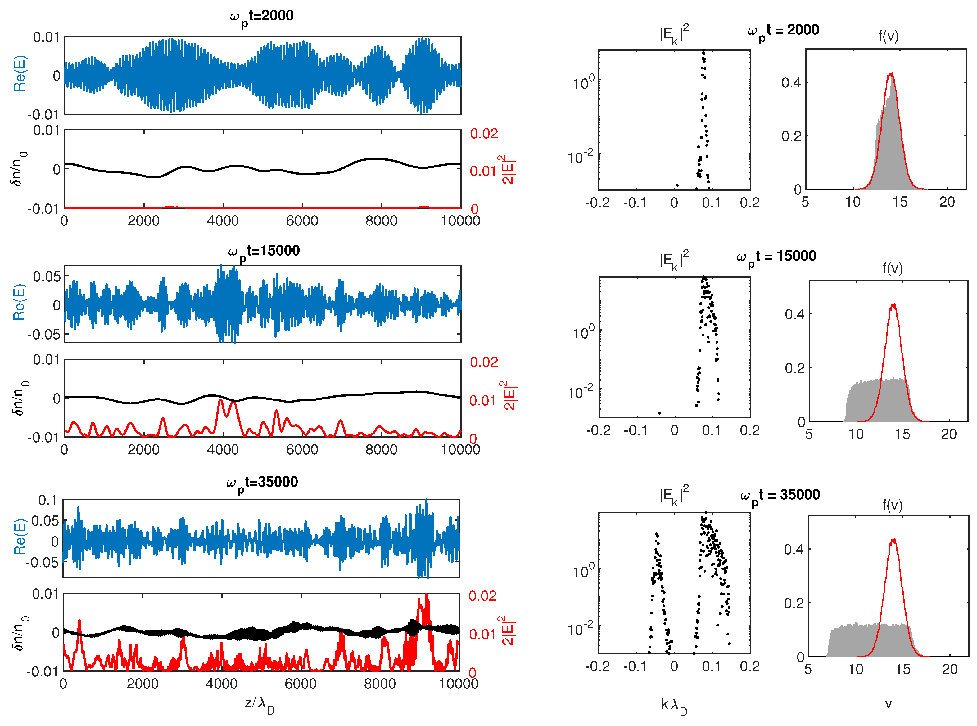
When the Langmuir wave packet is generated by an electron beam, the same spatial focusing phenomena occur. Figure 2, Figure 3 and Figure 4 show, for three different values of Δ n below and above the threshold ( Δ n = 0.001 Δ n s and Δ n = 0.01–0.03 > Δ n s , respectively) and three time moments, the spatial profiles of the Langmuir field envelope Re ( E ) , the energy density E 2 and the density fluctuations δ n / n 0 , as well as the corresponding beam velocity distributions f ( v ) and wave energy density spectra E k 2 . To complete the physical picture, Figure 5 shows the time variation of the total wave energy density W L = k E k 2 for different values Δ n = 0.001 0.04 together with the evolution of the beam dynamics for a quasi-homogeneous ( Δ n = 0.001 ) and a strongly inhomogeneous plasma ( Δ n = 0.04 ). When the plasma is quasi-homogeneous, the turbulent wave energy E 2 , as well as the field envelope, are distributed over the whole space and do not exhibit localized peaks (Figure 2, left column). The wave energy spectrum (Figure 2, middle column), which is peaked around the most unstable mode near k ω p / v b at early times ( ω p t 2000 ), broadens toward larger wavenumbers k (i.e., smaller phase velocities ω p / k ) due to the interactions of waves with the unstable beam ( ω p t 15,000), whereas the radiated Langmuir wave energy density W L grows up to saturation around a mean level (Figure 5a). The beam is decelerating (Figure 2, right column, and Figure 5c) according to the well known relaxation process described in the frame of the quasilinear theory [92], leading asymptotically to a velocity distribution in the form of a flattened plateau ( ω p t 35,000, see also Figure 6). It is worth mentioning here that another phenomenon appears starting from ω p t 35,000, which can occur independently of the presence of the inhomogeneities, i.e., the resonant decay of the Langmuir wave packet; indeed, the corresponding energy spectrum shows the appearance of backscattered waves with negative wavenumbers, whereas short-wavelength oscillations (i.e., ion acoustic waves generated during the decay process) manifest in the profile of the long-wavelength fluctuations δ n / n 0 (Figure 2, left). Note also that a small amount of accelerated particles is visible in the beam velocity distribution f ( v ) , beginning from ω p t 35,000 (see Figure 2 and Figure 6b); we will show in detail in the next sections that such effect is not due to the waves’ transformation processes on the inhomogeneities (which are here too weak) but to the second cascade of Langmuir waves’ decay producing daughter Langmuir waves able to accelerate beam particles.
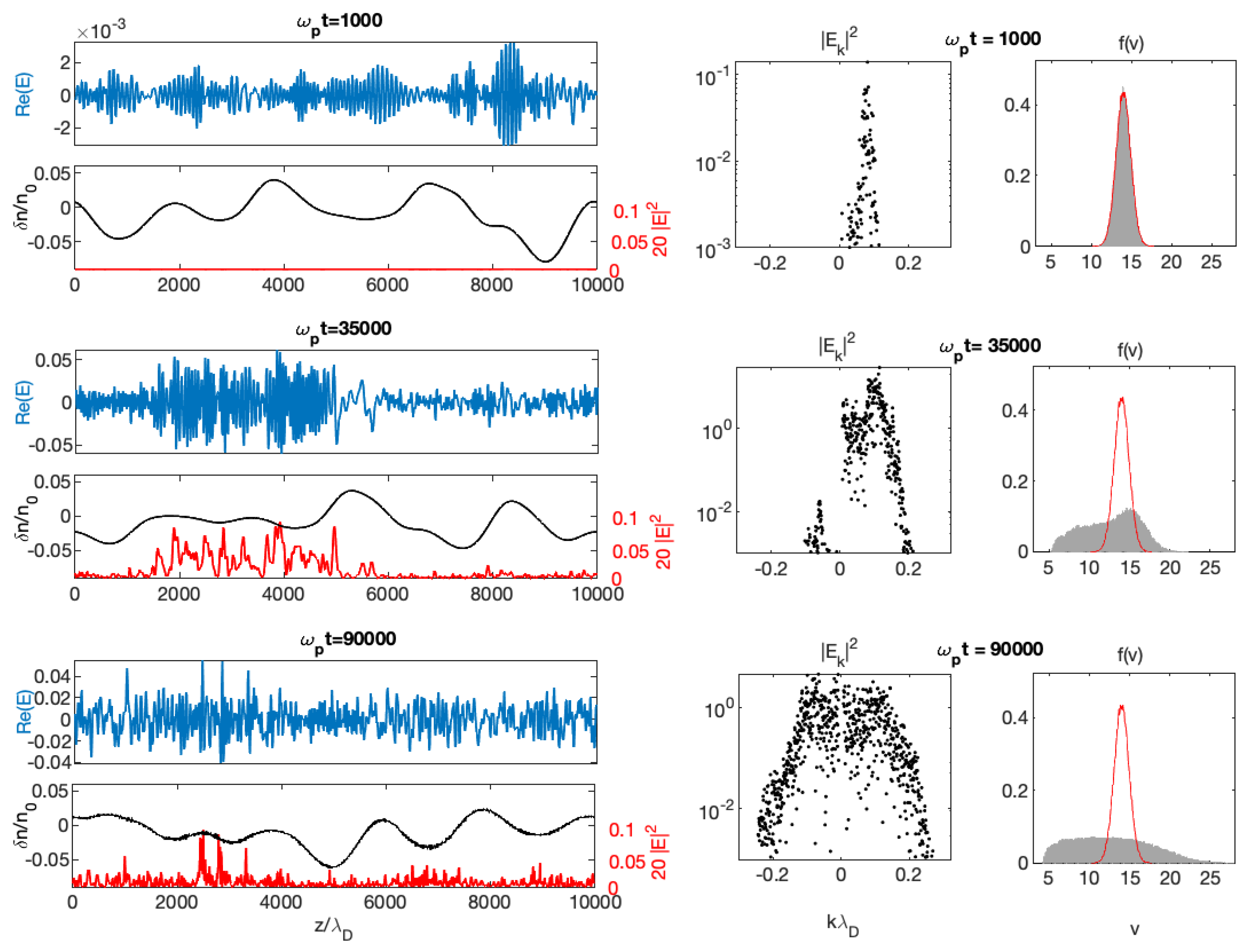
When Δ n exceeds the threshold Δ n s , the presence of density fluctuations impacts the beam relaxation and the wave turbulence it generates (Figure 3 and Figure 4, for Δ n = 0 . 01 and Δ n = 0 . 03 , respectively). Indeed, the wave energy density profile E 2 shows focused peaks resulting from a balance between the process of waves’ excitation by the beam, including their mutual interactions, and the transformation of the waves on the density fluctuations (Figure 3 and Figure 4, left columns, see at times ω p t 23,000 and ω p t 35,000, respectively). Moreover, these energy peaks are localized in some specific regions only, and not distributed over the full space as for the case of a quasi-homogeneous plasma (see the previous paragraph). As already mentioned above, such behavior results from the kinematic properties of the Langmuir waves’ propagation in a inhomogeneous plasma and is connected with the random character of the wave-particle resonance conditions ω k ω p = k v . As the existence of density fluctuations modifies randomly the local plasma frequency ω p and thus leads to shift randomly waves of wavenumber k and frequency ω k out of the resonance with the beam electrons of velocity v, the transfer of energy from the beam to the waves is strongly reduced and its relaxation is significantly slowed down (see Figure 3 and Figure 4, right columns, and Figure 5d, which shows the whole beam dynamics for a strongly inhomogeneous plasma with Δ n = 0.04 ). At the same time, the beam distribution f ( v ) is broadening not only toward lower but also higher velocities, and a tail of accelerated electrons is formed with velocities exceeding the beam velocity v b up to two times its value (see the right bottom panels of Figure 3 and Figure 4). This acceleration process, which will be discussed in detail below in a devoted section, partly results from a transfer of energy from the slower to the faster beam electrons during the transformation of the beam-driven waves on the density fluctuations. In the asymptotic stage of the relaxation, when the saturation stage of the instability is reached, the electron velocity distribution f ( v ) exhibits a quasi-plateau with a weak positive monotonic slope (see the right bottom panels of Figure 3 and Figure 4 and Figure 5c,d). On the other hand, the wave energy spectra E k 2 are shown to be significantly affected by the presence of density inhomogeneities (compare the middle columns of Figure 2, Figure 3 and Figure 4). Indeed, they are strongly broadened toward smaller as well as larger wavenumbers k, illustrating the simultaneous presence of waves excited by the beam instability (with larger k) and transformed by reflection, refraction and scattering on the density irregularities (smaller positive k and negative k). Please note that wave decay processes are also present, as will be discussed in the next section; decayed Langmuir waves are however not appearing in the spectra so clearly as in Figure 2, due to the simultaneous presence of scattered waves in the same ranges of wavenumbers.
Moreover, Figure 5b shows that for Δ n Δ n s , the rate of growth Ω W of the wave packet’s energy density W L decreases when Δ n increases, with a scaling law Ω W Δ n 2 . In this case, the saturation levels of W L , which depend weakly on Δ n , are significantly smaller than the saturation level reached in the case of homogeneous plasmas (i.e., for Δ n Δ n s , see the upper curve of Figure 5a), in accordance with the reduction of wave radiation by the beam due to the density fluctuations. Please note that we also will quantify in a next section the influence of Δ n on the kinetic energy density carried by the accelerated particles.
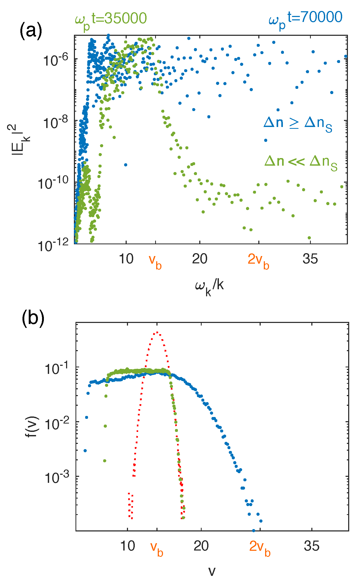
Let us now examine the asymptotic stage of the evolution. Figure 6 presents, for both cases Δ n Δ n s and Δ n Δ n s , the wave energy spectra E k 2 at asymptotic times, as a function of the resonant velocities v = ω k / k ω p / k > 3 v T above the thermal range. First, one can see that for a negligibly small average level of density fluctuations ( Δ n Δ n s ), the spectrum is broadened around the resonance condition ω p k v b , as a result of waves’ interactions with the beam electrons (Figure 6a, green points); only a small amount of beam energy is released to waves with large phase velocities above v b + Δ v b v b , so that only a very weak flux of accelerated particles appears. Second, in the velocity region between the beam velocity v b and the decelerating front velocity u f , i.e., for waves with phase velocities satisfying u f ω k / k < v b (here 8 ω k / k 14 ), the spectrum scales as E k 2 ω k / k 4 . This result is predicted by the quasilinear theory of the weak turbulence for homogeneous plasmas ([92]; see also [77]). On the contrary, when the density irregularities are sufficiently large ( Δ n Δ n s ), the spectrum is flattened asymptotically in the range ω k / k 3 v T , due to the transformations of the waves on the density inhomogeneities and to the random deviations from the resonance conditions (Figure 6a, blue points), as energy can be transported to larger phase velocities. Indeed waves with large phase velocities present amplitudes of about the same order of magnitude as those with phase velocities lying in the initial resonant velocity range 3 v T ω k / k v b . Therefore such waves with ω k / k v b can transfer energy to electrons with v v b through Landau damping and thus accelerate them. Moreover, the asymptotic velocity distribution f ( v ) superposed to the initial one (Figure 6b, blue and red curves, respectively) exhibits clearly the acceleration of electrons up to velocities v 2 v b . The decelerated part of the distribution f ( v ) exhibits a quasi-plateau in the region v < v b which is not flattened as in the case of a quasi-homogeneous plasma (Figure 6b, green curve); a weak and persistent gradient remains although the beam instability as well as the total wave energy density are saturated.

3.2. Wave Coupling and Decay Processes

In the solar wind, simultaneous observations of large amplitude Langmuir waves excited by electron beams associated with Type III bursts together with ion acoustic waves were performed [26]. Such phenomena were likely due to nonlinear processes of wave-wave interactions and, more precisely, to Langmuir wave decay. Besides, many examples of evidence or suspicion for resonant three-waves’ interactions were reported in front of planetary bow shocks as well as in the source regions of solar bursts. For example, the waveforms observed in front of the Jovian bow shock were interpreted in terms of beatings of Langmuir waves interacting with ion acoustic waves or density fluctuations [109,110]. More recently, evidence for three-waves’ interactions involving Langmuir waves was reported by several authors, concerning the Earth electron foreshock region and the source regions of Type III solar bursts [26,30,42,46,111,112,113,114,115,116,117]. At the same time, other works reported observations of electron beams or fluxes in the solar wind near the orbit of the Earth [30,32].
Recent measurements of the wave activity on board spacecraft such as Polar, Ulysses, Wind and Stereo revealed new features and details concerning the Langmuir wave turbulence. As an example, using several events observed by Stereo [118] that registered wave packets within a duration of 130 ms, some authors [116] argued that the threshold of the decay instability of a Langmuir wave into a daughter Langmuir wave and an ion acoustic wave was exceeded and presented Langmuir wave decays occurring during Type III solar bursts.Besides, Graham & Cairns [117] showed that about 40 % of the Langmuir waveforms measured by Stereo during Type III bursts can be consistent with the occurrence of such decay processes, involving in some cases several cascades. It is worth noting here that the Langmuir spectra and the wave profiles recorded by the Interball-2 satellite [119] in the inner regions of the terrestrial magnetosphere are very similar to those observed in the Earth foreshock as well as in the Type III solar bursts’ regions of the solar wind; the authors’ interpretation is based on the weak turbulence theory of scattering of beam-driven Langmuir waves on the external ion acoustic turbulence.
Large amplitude Langmuir waves L can decay into backscattered Langmuir waves L and ion sound waves S according to the channel L L + S . If the waves L transport enough energy, they can in turn decay as L L + S , producing Langmuir waves L (ion sound waves S ) propagating in the same direction as (in the inverse direction with respect to) the beam-driven waves L . Several such cascades can occur until the decay process becomes prohibited by kinematic effects. The decay L L + S allows to transfer wave energy from larger to smaller wavevectors k and, in particular, from k-regions where beam-driven mother waves are produced to regions (i) where resonant wave-particle phenomena can not occur (as non resonant domains where k < 0 ) or (ii) where the waves can damp and by the way release energy to beam electrons and accelerate them (when k < ω p / v b ). Above the instability threshold, the dynamics of the decay processes depends on the energy carried by the mother Langmuir waves as well as on the efficiency of its transfer to the daughter waves, effects which are both impacted by the wavelengths and the average level of the random density fluctuations.On the other hand, decay processes can significantly impact on the Langmuir waveforms’ features by modulating them or intensifying their clumpyness. Besides, the excitation of intense backscattered Langmuir waves can also lead to the emission of electromagnetic waves T near the frequency 2 ω p , via the fusion of two Langmuir waves according to the channel L + L T . Such process is assumed to be a first step in the mechanism of generation of Type III radiation at 2 ω p [120].
Numerical simulations were performed to study wave decay in weakly magnetized or non magnetized plasmas, mostly in the frame of the weak turbulence kinetic theory [56,59,121], for homogeneous plasmas and more seldom for plasmas with inhomogeneities, mainly in the form of density gradients [57]. So-called Vlasov codes and Particle-In-Cell (PIC) codes [59,60,61] were used as well as other ones developed in the frame of a fluid description based on the Zakharov equations [122]. Some of these works were applied to study Langmuir wave decay in solar wind plasmas and, particularly, in the source regions of Type III solar bursts or in the terrestrial foreshock.
Moreover, numerical simulations based on the theoretical modeling presented in Section 2 have shown that several cascades of resonant three-wave decay processes can occur in inhomogeneous plasmas typical of the solar wind where Langmuir turbulence is generated by energetic electron beams [74]. Indeed, in such plasmas, Langmuir waves can decay into backscattered Langmuir and ion acoustic waves if the average level of density fluctuations Δ n does not exceed a few percents (i.e., Δ n 0.04 ); otherwise the wave transformation processes on the density fluctuations usually overcome the decay processes. Decay was revealed in the low- and high-frequency wave energy spectra where peaks are excited at the wavenumbers of the mother and the daughter waves, in accordance with the waves’ resonance conditions. Besides, the growth rate of the ion acoustic wave energy was shown to fit the predictions of the theory of parametric decay for monochromatic waves and homogeneous plasmas, at least below Δ n 0.02 . A very good agreement was found concerning the wavenumbers of the waves involved in the decay processes when comparing the simulations’ results and the analytical predictions. This is related to the fact that the waves’ dispersion is not noticeably modified by the density irregularities.
Below the threshold Δ n s , three-wave decay processes can occur in plasmas with developed Langmuir turbulence; moreover they can be described within the frame of the weak turbulence theory for homogeneous plasmas [74]. In this case, the energy density carried by low-frequency as well as high-frequency waves is distributed quasi-uniformly in space and does not exhibit focused peaks isolated in some specific regions; wave decay is not a spatially localized process and can develop until its saturation stage.
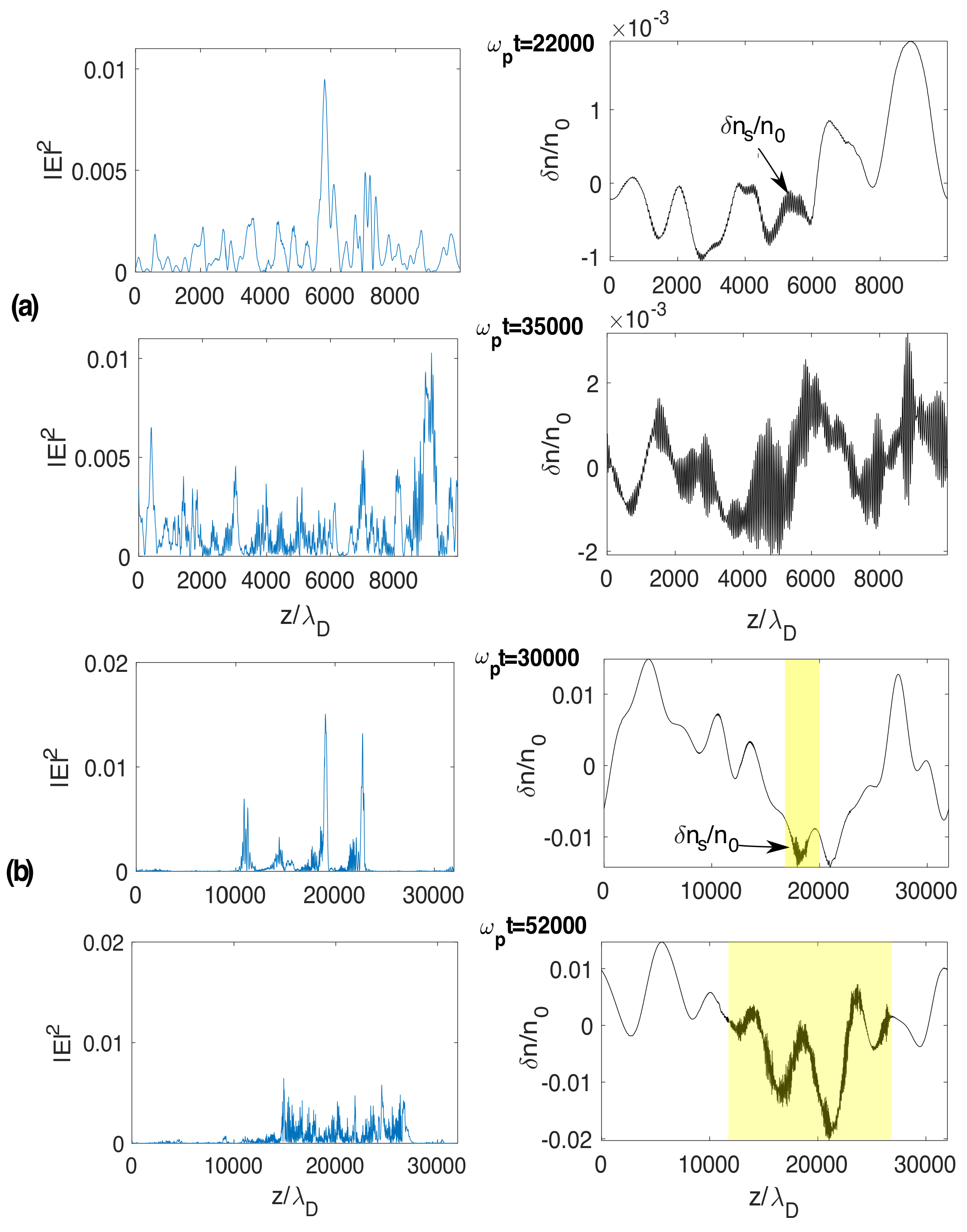
Figure 7a shows the corresponding space profiles of the Langmuir wave energy density E 2 and of the background plasma density fluctuations δ n / n 0 at two different times. One can see the appearance of short-wavelength density perturbations δ n s / n 0 of significant amplitudes (i.e., ion acoustic oscillations) which can be separated from the long-wavelength fluctuations δ n / n 0 by an adequate filtering procedure [74]. At asymptotic times, the Langmuir wave turbulence and the ion acoustic oscillations are extended over all space (see Figure 7a at ω p t = 35,000).
On the other side, when Δ n Δ n s , wave transformation phenomena as wave scattering, diffusion, refraction or reflection on the density irregularities compete with the decay processes which therefore take place in specific space-time locations imposed by the physical conditions and the dynamics of the system; indeed, one can see on Figure 7b that the wave energy density E 2 and the short-wavelength density perturbations δ n s / n 0 are localized in specific space-time regions, contrary to the case when Δ n < Δ n s (Figure 7a). Please note that these regions do not only concern the surrounding of reflection points on the density fluctuations’ humps where Langmuir wave energy can accumulate and focus before the start of the decay processes.
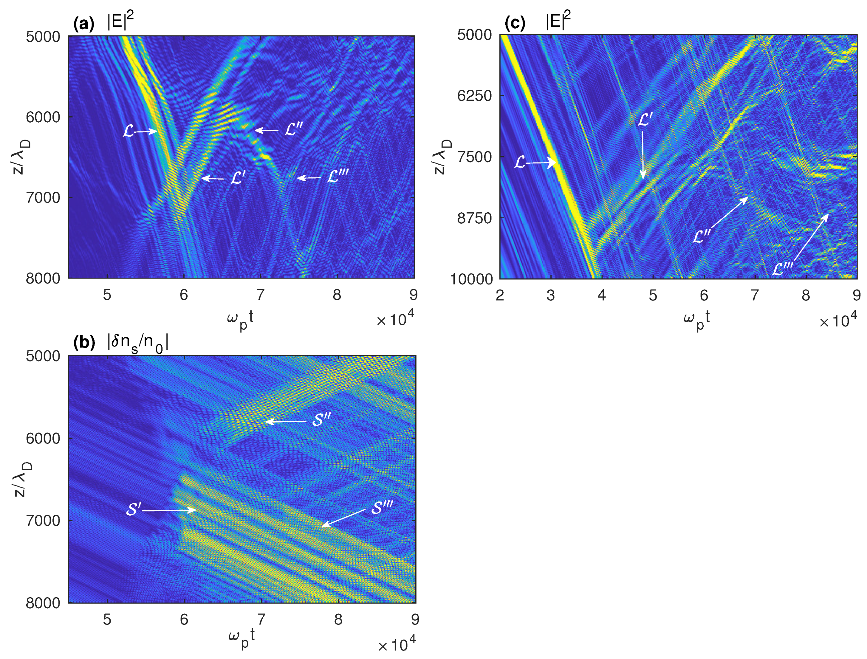
 Figure 8 and Figure 9 show for both cases Δ n < Δ n s and Δ n > Δ n s , respectively, the space-time dynamics of the Langmuir wave turbulence and the ion acoustic waves. Let us first discuss the case of a quasi-homogeneous plasma when Δ n is below the threshold Δ n s . Figure 8a,b present the space-time variations of the Langmuir wave energy density E 2 and of the short-wavelength density fluctuations | δ n s | / n 0 , respectively. The energy of the mother Langmuir waves L ( ω L , k L ) propagates with the group velocity v g , and one can observe the occurrence of multiple decays L L + S along all their paths (Figure 8a). The backscattered Langmuir waves L ( ω L , k L ) propagate with a group velocity of inverse sign and k L < 0 . Meanwhile ion acoustic waves S ( ω S , k S > 0 ) are produced which propagate with the velocity c s in the same direction as the mother Langmuir waves L (Figure 8b).
During the wave-wave interactions, the resonance conditions ω L = ω L + ω S and k L = k L + k S are shown to be verified. According to the theory developed for homogeneous plasmas [58,123], those are satisfied if k L k 0 k L and k S 2 k L k 0 , with k L ω p / v b and k 0 λ D = 2 c s / 3 v T 0 . 03 ; the Langmuir and ion acoustic wave dispersions are ω L ω p ( 1 + 3 k L 2 λ D 2 / 2 ) and ω S c s k S . The energy spectrum E k 2 of the Langmuir waves as a function of time (Figure 8c) shows peaks around k L and k L and, at sufficient large times, a peak around k L ; indeed, second decay cascades start to occur, according to the channel L L + S , producing Langmuir and acoustic waves L and S with k L k L 2 k 0 > 0 and k S 2 k L + 3 k 0 < 0 , i.e., with wavevectors of the same and the opposite signs as those of the mother waves L , respectively. Finally, the growths with time of the high- and low-frequency energy densities W L and W S are presented in Figure 8d, showing that the ion acoustic waves start to grow at the stage when the Langmuir waves’ energy density has reached a steady state. The linear growth rate of the decay instability, calculated using Figure 8d, is shown to be smaller but rather close to the analytical predictions obtained for monochromatic waves in homogeneous plasmas [74,124].
Let us now discuss the dynamics of wave decay for inhomogeneous plasmas with Δ n > Δ n s . In this case, the random variations of the local background plasma frequency and thus of the wave-wave resonance conditions explain why the influence of the density fluctuations on the nonlinear decay processes can be significant. In Figure 9a, we show the space-time variations of the Langmuir wave energy density E 2 , and one can see that the decay processes only occur in some specific domains. Indeed, as revealed by Figure 7b, the Langmuir wave energy is focused and localized (left panels), becoming more irregular and chaotic in the space regions where the ion acoustic waves have appeared (right panels), due to the processes of energy transfer and redistribution between the wavevectors’ scales occurring during wave decay. Moreover, the waves’ transformations on the density fluctuations (scattering, reflection, refraction) modify the propagation of their energy locally, so that they can loose part of it and thus have less possibility to encounter further decay processes. It is worth mentioning that the interactions between Langmuir and ion acoustic waves occur during short time durations. Indeed, as the group velocity v g of the Langmuir waves is typically much larger than that of the ion acoustic waves (which is equal to c s ), the decay processes stop due to kinematic effects and not to nonlinear wave saturation. This occurs when the faster Langmuir waves leave the regions where they locally interact with the slower ion acoustic waves.
The high- and low-frequency energy spectra are shown in Figure 9b,c at ω p t 89,000, when the decay processes are saturated, exhibiting peaks corresponding to the first decay L L + S and to the second cascade L L + S . Each wave packet excited can be identified clearly by a broadened peak centered with a good accuracy around the wave vectors k L , k L and k L (Figure 9b) as well as k S and k S (Figure 9c), whose analytical expressions are given above. Figure 9d shows the growth with time of the high- and low-frequency energy densities W L and W S , respectively; the significant growth of W S within the time interval ω p t 45,000–55,000 indicates that the ion acoustic waves S are growing with a rate around a few 10 4 ω p . Please note that moderate but significant ion and electron damping effects (electron and ion temperatures satisfy typically T e / T i 3 ) with rates γ i ω S and γ e ω p , which model the presence of nonthermal ion and electron tails, are present in the simulations shown in Figure 9, what explains the decrease of W L and W S at large times (Figure 9d). One can observe that such damping effects, even if significant, do not suppress the occurrence of the Langmuir wave decay processes. On the contrary, those can even be identified more clearly due to the disappearance of some Fourier components in the spectra.
Decay processes can lead to several cascades of energy transfer to waves with longer wavelengths [11]. Figure 10a–c present the space-time variations of the wave energy density E 2 and the short-wavelength density perturbations δ n s / n 0 when a third and last cascade occurs, a fourth cascade being not possible here due to the resonance conditions. One can observe the third decay cascade L L + S around ω p t 73,000 in the first example (Figure 10a,b), and near ω p t 80,000 in the second example including damping effects (Figure 10c). During the successive cascades L L + S , L L + S and L L + S , the absolute values of the Langmuir wavenumbers k L , k L and k L become smaller at each decay, starting from the wavenumber k L of the beam-driven Langmuir waves; due to the resonance conditions, the Langmuir wave products satisfy k L ( k 0 k L ) < 0 , k L ( k L 2 k 0 ) > 0 and k L ( 3 k 0 k L ) < 0 , whereas the ion acoustic daughter waves are characterized by the wavenumbers k S ( 2 k L k 0 ) > 0 , k S ( 2 k L + 3 k 0 ) < 0 and k S ( 2 k L 5 k 0 ) > 0 .
Whereas in quasi-homogeneous plasmas decay processes occur usually when the beam is almost totally relaxed, they can start in inhomogeneous plasmas much before the beam relaxation is complete, due to the wave energy focusing and reflection processes. In this case, when the presence of density fluctuations enhances the possibility to generate counterpropagating Langmuir waves, interferences between Langmuir waves become more frequent. In some cases reflection effects can favor the appearance of decay processes, that is, increase their efficiency in the early stage, due to coupling between Langmuir waves of amplitudes above the thermal level. However, in general, the larger Δ n is (and the smaller the density fluctuations’ wavelengths), the rarer the decay processes become, as they can be overcome by transformation effects of waves on the density inhomogeneities as well as by reflection effects. For large Δ n significantly above Δ n s , wave decay occurs only rarely and under specific local conditions; indeed, the scattering of the waves on the irregularities, which has a much shorter characteristic time scale than the wave decay, destroys the coherency between the waves required for decay.As an example, wave decay can be observed in the present simulations up to Δ n 0.03 , although it is obscured by reflection phenomena, but can not be detected at Δ n 0.03–0.04.
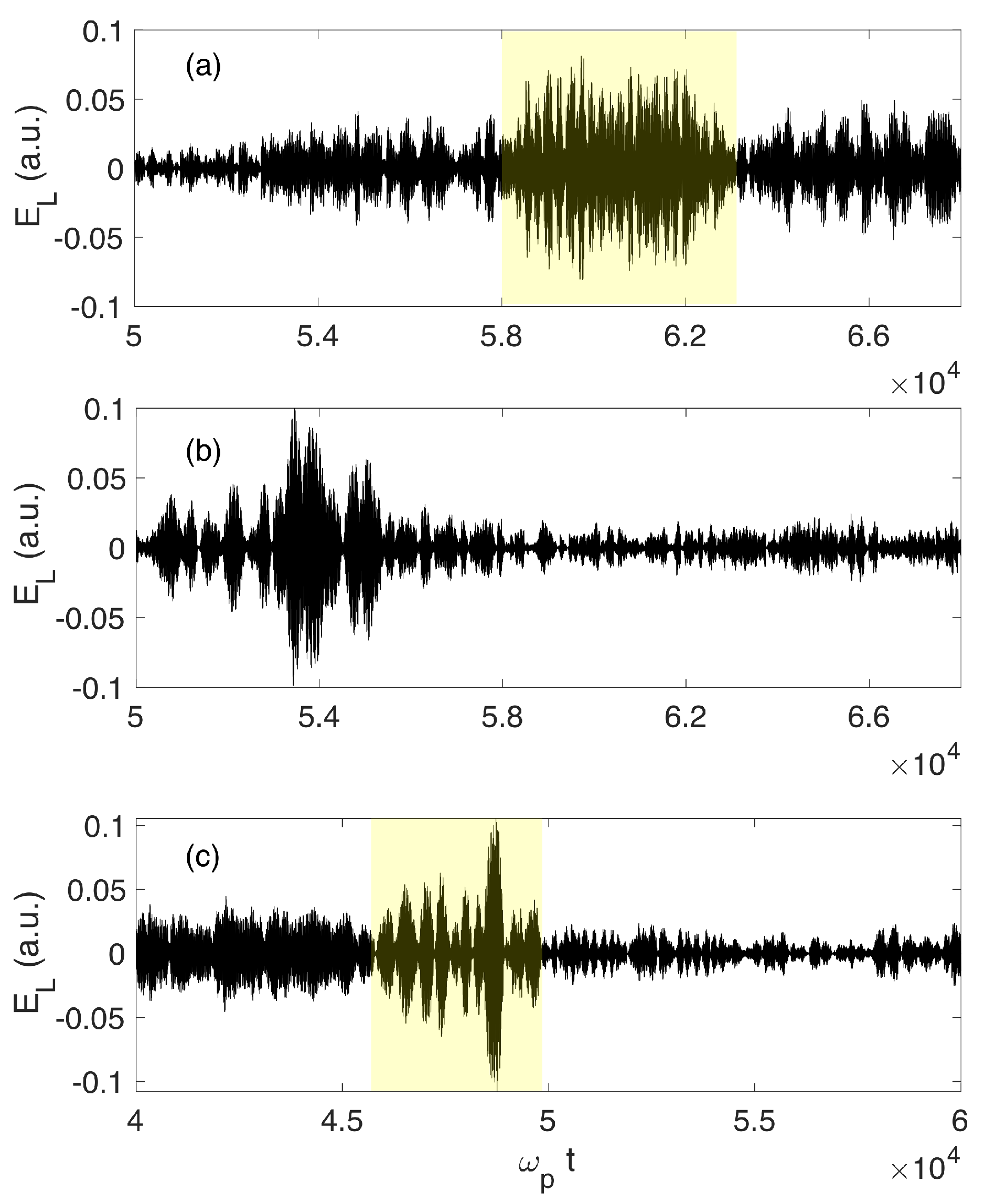
As discussed above, second decay cascades and more can be observed which redistribute wave energy between the different k-scales of the Langmuir wave turbulence. This leads to the appearance of modulation features in the Langmuir waveforms, which can be shaped in clumps due to three-wave decay processes. The waveforms E L t = Re k E k t exp i k z v S t i ω p t , calculated numerically and registered as a function of time by a virtual satellite passing through a space-time region where a three-waves decay process occurs, exhibit specific modulation features revealing beatings between waves (Figure 11a); when the same satellite does not cross this region, such modulation is no more visible (Figure 11b). Figure 11c presents a Langmuir waveform recorded by another virtual spacecraft travelling in a strongly inhomogeneous plasma ( Δ n 0.03 ) through an area where wave decay occurs, which exhibits characteristic modulation features. Such numerical simulations’ results are in agreement with observations by the Stereo satellite showing the same kind of modulated structures during the occurrence of wave decay processes [125].

3.3. Particle Acceleration Processes

It is well known that an electron beam emitting Langmuir waves can reabsorb some part of the energy it radiates. As a result, this beam is able to emit moderate levels of wave turbulence and to transport energy over large distances far from its emission source before being thermalized. During such processes, the acceleration of particles plays a determinant role, which is different depending on whether the plasma is inhomogeneous or not and on the nature of inhomogeneities. Simulations involving large scale density inhomogeneities have demonstrated that beam electrons can be accelerated when propagating into a plasma of increasing density [126,127]. Moreover PIC simulations have shown that accelerated electrons appear during the nonlinear evolution of a beam-plasma system [88] even if the background plasma is initially homogeneous.
On the other side, when the plasma involves random density fluctuations, the appearance of accelerated particles results from two different phenomena: (i) the scattering of the waves on the fluctuating density inhomogeneities [10,53,57] and (ii) the damping of Langmuir waves coming from the second cascade of the electrostatic decay [67], which can transfer energy to some beam particles through resonant wave-particle interactions. The first process is not efficient when the plasma is weakly inhomogeneous ( Δ n Δ n s ) ; but, when Δ n exceeds the threshold Δ n s , it can lead to a population of accelerated particles carrying significant density and energy. The second process can be effective even if the plasma is quasi-homogeneous ( Δ n Δ n s ), but tends to be suppressed at high Δ n > Δ n s due to the rare occurrence, at these conditions, of Langmuir wave decays and their second cascades [74]. Moreover, these two acceleration mechanisms occur on different time scales, the second one developing typically after the first one has reached its saturation stage. In particular, it is important to understand how the second wave decay cascade and the wave transformation (scattering) processes can work together to accelerate beam electrons during two successive stages.
It was shown that the Langmuir waves coming from the second cascade of the electrostatic decay L L + S can accelerate beam electrons up to kinetic energies and velocities exceeding half the initial beam energy and two times the beam velocity v b , respectively [67,69]. Besides, this process can be particularly effective (and sometimes can only occur) if there exists beforehand a sufficient amount of particles with velocities extending over a few Δ v b above v b ( Δ v b is the beam thermal velocity). This can be realized as a result of Langmuir waves’ transformations on the background plasma density fluctuations, which allow energy to be transported to waves of higher phase velocities and then to be released to electrons with velocities v > v b . If the phase velocities of the waves coming from the second cascade of the decay are lying between v b and 2 3 v b , such waves can transfer resonantly their energy to the firstly accelerated electrons which are thus again accelerated.Such conditions can be met in typical solar wind plasmas if the beam velocity v b does not exceed about 35 times the plasma thermal velocity v T [67]. Thus the processes of waves’ transformations on density fluctuations can prepare the accelerated beam electrons to a second acceleration stage by waves produced through a decay channel.
We remind readers here that the daughter Langmuir waves L ( L ) produced by the first (second) decay cascade propagate in the inverse direction to (the same direction as) the mother wave L , i.e., as the electron beam (see also the previous section). As a consequence, the waves L coming from the first decay cascade L L + S can not be resonant with the beam electrons (as their phase velocities are negative), contrary to the waves L produced by the second cascade L L + S . Besides, in accordance with the weak turbulence theory, the succession of cascades allows the transport of energy to larger phase velocities. In this view the important question arises under what conditions the waves L , which have absorbed part of energy of the waves L via wave-wave interactions, can be damped and loose part of their energy to beam electrons and thus accelerate them. Then, it is essential to distinguish the different acceleration mechanisms one from the others, to estimate their own contributions, to find the specific conditions under which they can compete to eventually favor or reduce acceleration, and to determine whether those are consistent with the solar wind parameters typical of the source regions of Type III solar bursts or of the Earth foreshock.
Figure 12a,b show the time variations, for different values of Δ n , of the Langmuir wave energy density W L , the beam kinetic energy density K t , as well as the energy density K a c and the density n a c carried by the population of accelerated particles, i.e., with velocities above the value v a c v b + Δ v b ; K t , K a c and n a c are normalized by the initial beam kinetic energy density K 0 and beam density n b , respectively. As expected, the growth of W L (Figure 12a) is accompanied by the decrease of K t (Figure 12b), the beam loosing energy when radiating Langmuir wave turbulence. The variations of energy are different for small Δ n below the threshold Δ n s and above it. Indeed, for Δ n Δ n s , the beam kinetic energy experiences a large loss (around 30% of its initial energy at Δ n = 0.001 , Figure 12b), producing a high level of Langmuir wave turbulence (see the corresponding saturation level of W L in Figure 12a). When Δ n > Δ n s , the Langmuir waves’ emission efficiency is significantly reduced as a result of the random violation of the wave-particle resonance conditions and of the reabsorption of the wave energy by the beam; at large Δ n = 0.04 , the beam loss is eventually around 5%, in agreement with its ability to propagate over long distances in the solar wind (see Figure 12b at asymptotic time). Wave energy growth and resulting loss of beam energy occur mostly at ω p t 50,000 before the saturation stage that starts near ω p t 50,000. For Δ n > Δ n s , wave energy is transferred from the Langmuir waves L excited by the beam to modes of smaller wavevectors, as a result of waves’ transformation effects on the density fluctuations; therefore n a c and K a c strongly increase (Figure 12c,d). Then, during the saturation stage, they continue to increase but at a much slower rate, as the waves’ transformation effects are not fully achieved. On the other hand, for Δ n Δ n s , the growth of n a c and K a c is mostly due to the occurrence of the second decay cascade process, that begins to be effective around ω p t 50,000, when Langmuir waves L with phase velocities v φ v a c are produced by the second decay cascade (see Figure 12c,d for Δ n = 0.001 ).
Let us define W L , a c as the wave energy density carried by the Langmuir waves with phase velocities v φ > v a c . For Δ n = 0.001 Δ n s and at large times ω p t 50,000, W L , a c and W L , a c / W L are growing and saturating (Figure 12e,f); these growths are only due to acceleration by damping of the decayed waves L ; the saturation level of W L , a c / W L oscillates around 0.4 . For Δ n = 0.02 > Δ n s , the two phenomena leading to particle acceleration occur both at ω p t 50,000, i.e., the transformation of waves on the density fluctuations and the second decay cascade process (which takes place only for ω p t 50,000). For Δ n > Δ n s , the larger Δ n , the larger the fraction W L , a c / W L of wave energy transferred during the waves’ transformation processes to waves with v φ v a c ; in the same conditions, the smaller Δ n , the larger the fraction W L , a c / W L transferred by the second decay cascade process to waves with v φ v a c .
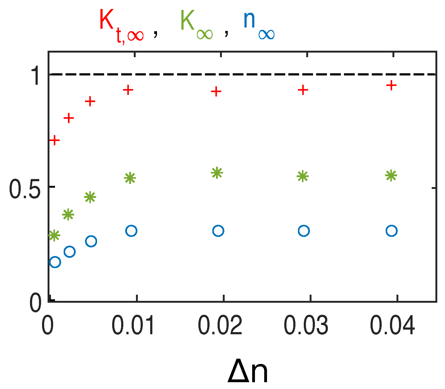
Figure 13 shows the variation with Δ n of the asymptotic values n , K , and K t , of n a c , K a c , and K t . One can observe that K and n increase with Δ n up to stabilization. For Δ n Δ n s 0.008 , n and K depend linearly on Δ n ; on the contrary, n , K c s t when Δ n Δ n s . The kinetic energy and the density of the accelerated electrons can reach up to 60 % and 30 % of the initial beam energy and density, respectively, as the maxima reached are K 0.6 and n 0.3 . According to the variation of K t , with Δ n , one can see that for Δ n 0.001 Δ n s ( Δ n 0.04 Δ n s ), the beam has lost eventually 30 % ( 5 % ) of its energy, as the waves’ transformations on the density fluctuations prevent the beam from loosing energy at large Δ n (see also Figure 12b). Indeed, as the tail of accelerated electrons can reabsorb part of the energy that the decelerating beam looses, the net energy lost due to radiation into wave energy is very small when density fluctuations exist and, in particular, when they are large. Such reabsorption allows the beam to conserve its kinetic energy during a significantly more long time during its propagation in inhomogeneous plasmas than in homogeneous ones. Note that the accelerated electron tail can extend asymptotically up to around 2–3 times the initial beam velocity v b , whatever the value of Δ n is.
Figure 14a shows that when Δ n increases, the asymptotic values of the saturated energy density W ¯ ( W ¯ a c = W ¯ ( v φ > v a c ) ) of all the Langmuir waves (of the Langmuir waves with phase velocities satisfying v a c v φ ( 2 3 ) v b ) decrease. For Δ n Δ n s 0.008 , W ¯ and W ¯ a c depend weakly on Δ n . As expected, W ¯ a c is noticeably smaller than W ¯ ; when Δ n < Δ n s , this results from the fact that as waves’ transformation effects are weak, no noticeable amount of energy is transferred to the waves with v φ > v a c ; when Δ n > Δ n s , the reason is that the Langmuir waves with v φ > v a c have released through damping, to the particles with velocities v v a c , a part of their energy gained during their transformation processes on the density fluctuations. One can see that W ¯ a c and W ¯ decrease when the normalized velocity width Δ V characterizing the distribution f ( v ) at v > v b increases (Figure 14c); indeed, for very low saturation levels W ¯ at large Δ n , the energy transported by the waves has been in part absorbed by the electrons, which are then accelerated. The variation of Δ V (calculated at the saturation stage) with Δ n is shown in Figure 14b, when the two acceleration mechanisms are taken into account indistinctly. One can see that Δ V Δ v b 1.5 v T for small Δ n < Δ n s , and that it increases with Δ n up to Δ V 4 Δ v b when Δ n = 0.04 > Δ n s . In the former case, the broadening of the distribution f ( v ) mainly results from the second cascade of the Langmuir decay and, in the latter case, this process contributes more weakly to the growth of Δ V , so that the wave transformation phenomena on the density fluctuations are predominant.
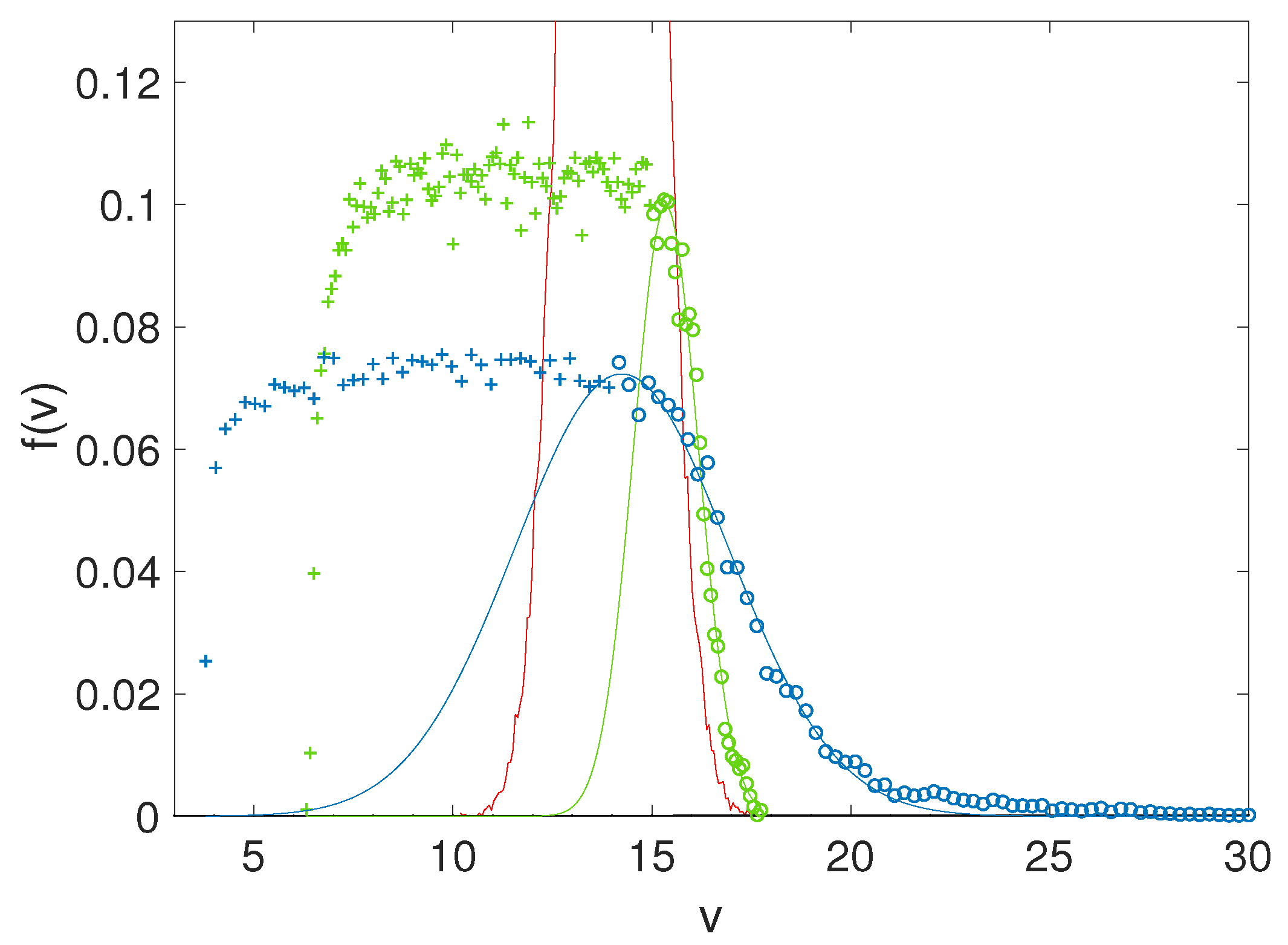
For a quasi-homogeneous plasma with Δ n Δ n s , Figure 15 shows the electron distribution f ( v ) at three different moments of the beam dynamics, i.e., at t = 0 , at the time ω p t = 47,500 when the transformation processes of the waves on the inhomogeneities are saturated (green), and at ω p t 170,000 when the second decay process occurs (blue); the distributions are superposed to their interpolations by Gaussians centered at v v b + Δ v b . One observes that as Δ n is small, particles are weakly accelerated by the processes of waves’ transformations. However, another acceleration mechanism takes place due to the damping of the waves L . One can see that at ω p t 170,000 and v 22 , the tail of f ( v ) is denser than that of the Gaussian distribution. Indeed, the second decay cascade process is not totally saturated at this stage, as the spectrum of the Langmuir waves L significantly varies within the velocity domain considered, as a result of local resonant energy exchanges between the tail electrons and the waves. In this case the accelerated electron tail deviates locally from the Gaussian behavior. However, when wave saturation is established, the tail distribution is Gaussian, due to the fact that in the velocity range above v b , the velocity diffusion coefficients D ( v ) of electrons are quasi-constant at saturation [68,77] (see also the next section). Note that the quasilinear theory predicts this kind of behavior in the velocity range where the waves’ energy exchanges with the particles are not significant. Moreover, when the two processes responsible for electron acceleration are fully saturated so that energy exchanges between particles and waves are very weak asymptotically, the coefficients D ( v ) can become quasi-constant at v > v b even when the plasma is inhomogeneous.
Let us now characterize the population of accelerated electrons. Figure 16a shows, for Δ n 0.01 , the variation with time of the normalized density n a c and kinetic energy density K a c of a population of electrons accelerated successively by the two acceleration processes. Indeed, one observes two stages in the evolution of K a c : the first growth (up to K a c 0.2 ), occurring at times ω p t 15,000, is due to the scattering of the waves on the inhomogeneities; during a second period from ω p t 70,000 to ω p t 100,000, K a c grows up to K a c 0.4 , due to the development of the second decay cascade, and reaches eventually around 0.55 . The density n a c follows the same behavior, with smaller growths however, reaching a maximum around n a c 0.3 . Then, in the asymptotic time, almost 60 % of the initial beam energy is carried by the accelerated electrons which constitute 30 % of the beam density. Without the second decay cascade, only 15–20% of the beam electrons’ density would carry 25 % of the initial beam energy. So, the waves L are able to reaccelerate strongly the electron population firstly accelerated due to the waves’ transformation effects.
Figure 16b shows the time variations of the normalized density n < a c and kinetic energy density K < a c of the beam electrons with velocities v smaller than v a c , together with the absolute value K l = 1 K a c + K < a c of the energy lost by the beam. One observes that n < a c decreases and n a c + n < a c 1 during all the evolution; K l follows qualitatively the variation of W L , as the beam instability generates Langmuir waves. The growth of K l (energy mostly absorbed by the Langmuir waves) at the early times corresponds roughly to the growth of the energy K a c of the electrons accelerated as a result of transformation effects of the waves driven by the beam. A second growth of K a c accompanies the further decrease of K l ; indeed, Langmuir waves damp and electrons absorb their energy. At the same time the beam electrons with v < v a c continue to loose energy ( K < a c decreases within the same time range), and the evolution of f ( v ) confirms (as the decrease of n < a c ) that electrons with such velocities can be accelerated and enter the domain v > v a c , whereas contributing to the growth of K a c . Indeed, due to the fact that f / v < 0 for v > v b , the waves L can damp and accelerate electrons, which can leave the range v v b , forming step by step a velocity distribution with a negative slope in this region; this effect continues to work as time increases. This explains the loss of beam energy K < a c as well as the appearance of the negative slope required for effective damping at v v b . At large times, Langmuir waves with phase velocities v φ v b can also experience damping; nevertheless, their ability to increase the energy of the accelerated electrons is weaker than that of the waves L produced by the second decay cascade process.
In summary, for a quasi-homogeneous plasma, the beam can loose up to half its initial kinetic energy, generating a high level of Langmuir wave turbulence. Beam electrons can be accelerated only by the Langmuir waves coming from the second cascade of the Langmuir wave decay. This population can absorb a large part of the initial beam energy, owing to the transfer of energy via wave-wave resonant coupling; indeed, mother Langmuir waves excited directly by the beam can decay into daughter Langmuir waves of phase velocities larger than the beam average velocity. Then the beam can reabsorb a significant part of the energy that it lost, even if the plasma is quasi-homogeneous. For a inhomogeneous plasma, the presence of density fluctuations as well as the reabsorption of wave energy by the beam reduce significantly the efficiency of Langmuir wave emission. In this case, a small part of its energy is lost by the beam at the asymptotic stage (less than 10 % ), so that it can propagate over long distances in the plasma. The two acceleration mechanisms resulting (i) from the second Langmuir decay cascade and (ii) from the waves’ transformations on the density fluctuations both lead to the formation of a tail of accelerated particles that can reabsorb the radiated Langmuir wave energy through resonant wave-particle interactions, limiting the energy loss of the beam.

3.4. Particle Diffusion Processes

Quasilinear theory [128,129] is one of the approaches used to study Type III solar bursts driven by electron beams; in particular, it provides analytic expressions for the velocity diffusion coefficients D ( v ) of particles moving in homogeneous plasmas. As the collision frequency is much smaller than the other characteristic frequencies in the solar wind, the velocity perturbations of the beam electrons are mostly due to the quasilinear diffusion. In the first attempt to extent this theory to inhomogeneous plasmas, some authors [53] assumed that the characteristic wavelengths of the background density fluctuations significantly exceeded those of the Langmuir waves and that most of these waves were trapped in density troughs. Such assumptions are however too strong as Langmuir turbulence involves waves that propagate freely over the density holes. Indeed actual effects as scattering and wave reflection on the density irregularities can not be neglected as they play a determinant role.
The diffusive properties of particles’ motion in wave packets were investigated in homogeneous plasmas owing to numerical simulations [77,130,131]. Some authors studied particle diffusion in given packets of waves with random phases and found discrepancies between the velocity diffusion coefficients calculated numerically and those predicted by the quasilinear theory [132,133,134,135,136,137]. Besides, the non classical nature of the diffusion at work was revealed [138,139] as, for example, the nonlinear time dependence of the particles’ mean-square velocity variations ( Δ v ) 2 . Another approach was proposed by the authors [77] as an alternative to the quasilinear theory. It consists in performing numerical simulations based on a self-consistent Hamiltonian model of resonant wave–particle interactions. In this frame, many individual test particles’ trajectories were calculated and analyzed owing to statistical algorithms and methods. Results obtained were close to the predictions of the quasilinear theory; particularly, it was shown that the velocity diffusion coefficients D ( v ) resulting from the analysis of a huge number of long-time trajectories in homogeneous plasmas agree on the whole with those obtained by this theory, even if some essential differences could be revealed [77].
A similar approach was also developed by the authors for the case of plasmas with developed Langmuir turbulence and random density fluctuations [68]. The presence of randomly fluctuating inhomogeneities affects the character and the nature of the beam electrons’ motion in the Langmuir wave packets, so that the diffusion processes are significantly modified; then the question arises to what extent the quasilinear theory remains able to describe these phenomena. Moreover, the determination of the velocity diffusion coefficients allows estimating the impact of such inhomogeneities on the dynamics of the beam relaxation, i.e., of the populations of beam electrons accelerated as a result of wave scattering on the density fluctuations or of nonlinear effects, or decelerated due to the generation of Langmuir wave turbulence. Therefore the resonance broadening effects due to waves’ transformations on the density inhomogeneities were studied owing to numerical simulations [68]. Such problems were also considered in the frame of a statistical and analytical model [63] or by using the quasilinear theory with wave diffusion coefficients, involving resonance broadening phenomena [140].
The authors [68] performed a statistical analysis of several thousands of test particles’ trajectories v t calculated for different parameters of beams and initial density fluctuations’ distributions. It was shown to be an effective tool for describing the diffusion processes at work in a inhomogeneous plasma, even if it required to analyze a huge amount of particles’ trajectories and to determine large series of stochastic variables while choosing adequate time scale parameters ensuring its reliability. Such study was aimed, first, at determining the probability distribution functions (PDFs) of the velocity variations δ v τ ( t ) = v t v t τ during the steady stage of the system’s evolution ( τ is a short time interval) and, second, using these distributions, at calculating the corresponding mean-square velocity displacements as a function of τ in order to determine the velocity diffusion coefficients. So, for each electron trajectory v t , a random sequence of velocity increments δ v τ ( t ) was built for t t 0 , where t 0 is the time when the fluctuations of the mean spectral energy density E k 2 become negligible. The autocorrelation sequence R ( τ ) = δ v τ ( t ) δ v τ ( t τ ) of the random process δ v τ showed that correlations almost disappear on a time scale of a few plasma periods ω p 1 , so that the statistical properties of the increments δ v τ ( t ) were almost independent on the time t.
The trajectories v ( t ) of typical test particles are shown in Figure 17 within a time interval Δ T in the saturation stage of the Langmuir wave energy density, together with their corresponding velocity variations δ v τ ( t ) = v t v t τ , in the case of an inhomogeneous plasma (Figure 17a,b) and a homogeneous plasma (Figure 17c,d). In the former case, one can observe sharp velocity jumps which appear to be localized (as the wave spectral energy); indeed, the energy of a wave packet scattering on a density hump focuses, whereas fast wave energy transfers occur through the wavevectors’ scales and, consequently, the electron motion exhibits sharp velocity jumps. In a homogeneous plasma, such jumps are much more seldom and smaller (Figure 17c,d). Please note that the small time τ ( τ Δ T ) has to be chosen large enough to ensure a sufficient number of interactions between particles and waves, leading to diffusion.
Figure 18a,b presents, for an inhomogeneous plasma with Δ n = 0.01 , two PDFs P δ v τ of the velocity increments δ v τ ( t ) , for two intervals Δ T and several values of τ . For comparison, we present in Figure 18c a typical PDF P h δ v τ obtained in the case of a homogeneous plasma. The function P δ v τ shows at large δ v τ higher values than P h δ v τ , i.e., larger probabilities for large velocity increments when the plasma is inhomogeneous, what is in agreement with the sharp and large velocity variations observed in the particle trajectories (see Figure 17a,d). At small and moderate values of increments, P h δ v τ can be approximated by a Gaussian function and, at large δ v τ , by an exponential function (Figure 18c). For the inhomogeneous plasma, P δ v τ is better fitted by a sum of two Gaussian functions for moderate values of δ v τ and by the sum of a Gaussian and a power functions for larger δ v τ , as illustrated in Figure 18b. So, in both cases, the PDFs show non Gaussian behaviors at large δ v τ , that is, diversions from the normal diffusion process at large velocity increments. Such non-Gaussian tails do not influence quantitatively on the velocity diffusion coefficients, due to their low probability, but they play an important role on the qualitative point of view, as discussed hereafter. Finally, one can see that the mean-square displacement δ v τ 2 obtained varies linearly with τ , for both the homogeneous and the inhomogeneous plasma cases (see the inserts in Figure 18a,c).
In a homogeneous plasma, the amplitudes of the waves at saturation exhibit only slight variations with time, and the study of the diffusion processes can be reduced to the problem of particles’ motion in a given wave packet. On the contrary, when the plasma is inhomogeneous, the Langmuir spectra at saturation show significant fluctuations with time so that we have to choose Δ T within the saturation stage when the total energy density is quasi-constant and use only time-averaged spectra, i.e., time-averaged values of | E k | 2 . Then, the mean square displacement used to determine the diffusion coefficient D ( v ) = Δ v τ 2 / 2 τ is obtained by averaging δ v τ 2 using the PDF P δ v τ
Δ v τ 2 = P δ v τ δ v τ 2 d δ v τ .
Figure 19a,b show the linear variation of the maximum value of Δ v τ 2 as a function of τ (note that the non maximum values present the same behavior) as well as the dependence of the corresponding diffusion coefficient D ( v ) on the waves’ phase velocity ω k / k ω p / k , for different values of τ , superposed to the analytical prediction D t h ( v ) of the quasilinear theory [92]
D t h ( v i ) = E k i 2 2 δ k i v i = v i E k i 2 2 ω p δ v i ,
where the square of the electric field Fourier component E k i 2 at the wave-particle resonance condition k i = ω p / v i is calculated using the time-averaged value of E k = ω p / v 2 computed over the interval Δ T ; δ v i and δ k i = δ ω p / v i = δ v i ω p / v i 2 are the distances between adjacent waves in the velocity’s and the wavevector’s space, respectively. Figure 19c,d present two other typical examples obtained for inhomogeneous plasmas with different average levels Δ n and time intervals Δ T .
Simulation results show that the diffusion coefficients D ( v ) = Δ v τ 2 / 2 τ derived owing to the statistical method mainly depend on the Langmuir wave spectra. Moreover they are shown to be in good agreement with the analytical predictions D t h ( v ) of the quasilinear theory, except of some quantitative differences observed in the range of phase velocities corresponding to short wavelengths, where the wave energy is mostly concentrated and where the coefficients D ( v ) are smaller than the coefficients D t h ( v ) . Such discrepancies, which are vanishingly small when the plasma is homogeneous [77], result from the transformation effects of the waves on the plasma density inhomogeneities (scattering, reflection, refraction, tunneling, etc.). Indeed, simulations reveal that the Langmuir waves’ phases oscillate faster in this velocity domain where most of energy is accumulated, so that the resonance conditions between particles and waves are more strongly violated. Therefore, the actual diffusion coefficients D ( v ) are smaller than the theoretical values D t h ( v ) .So the fluctacting inhomogeneities, as they significantly impact the Langmuir turbulence level itself, influence also on the diffusion coefficients. Indeed the saturation level and the rate of growth of the Langmuir energy density W L decrease when Δ n increases; the average level E k 2 of the spectral energy density shows also such behavior, explaining why the diffusion coefficients are eventually depending on the presence of inhomogeneities.
Moreover, other differences with the quasilinear theory can be observed. The tail of D ( v ) toward larger velocities is much longer and denser when the plasma is inhomogeneous than when it is homogeneous: indeed, due to the interactions between the beam driven Langmuir waves and the density fluctuations, waves with phase velocities up to 2 3 v b appear. As a consequence, a population of accelerated beam electrons is formed (see the previous section). In the velocity region v b v ( 2 3 ) v b the coefficient D ( v ) is quasi-constant, in agreement with the fact that, asymptotically, the tail of the electron velocity distribution exhibits a Gaussian shape. Indeed, the probability of large jumps of velocity in the electrons’ trajectories, i.e., characterized by a velocity variation larger than about 2 3 ( D τ ) 1 / 2 , essentially exceeds the probability of a Gaussian distribution. Such jumps are connected to the transformation phenomena of Langmuir waves on the plasma density inhomogeneities; moreover, their role is determinant as they modify the nature of the diffusion processes, which appear to be no more classical. These higher order effects are responsible for the discrepancies observed between the simulation results and the quasilinear theory, which does not involve them in its perturbative approach.

3.5. Langmuir Waveforms: Simulations and Space Observations

Satellites commonly measured in the solar wind modulated Langmuir waves associated with Type III solar bursts (e.g., [21,30,31,32,33,34,35], and references therein). Observations revealed bursty wave packets clumped into spikes. Moreover, intense Langmuir waveforms exhibiting electric field peaks up to 10 2 –10 3 times the mean were reported [8,26,42,96,97,141]. More recently, in situ observations of high time resolution performed by the spacecraft Stereo [118] showed that Langmuir waveforms often appear as clumpy packets with electric field amplitudes up to a few tens of mV/m and with durations of a few milliseconds [35,97,142]. With registration times ten times larger than onboard earlier missions (65 ms to 2 s), Stereo recorded Langmuir waveforms appearing mainly as multiple bursts’ events, more than well shaped isolated structures with one or a few humps.
Several attempts to explain the physical processes at the origin of such modulations have been proposed. Particularly, some authors [1] argued that the solar wind density fluctuations may be responsible for such effects, in the frame of transformations of Langmuir waves on the irregularities or stochastic growth effects [143]. They proposed that the appearance of the clumpy structures could result from a significant decrease of the bump-on-tail instability due to density fluctuations with length scales about the waves’ spatial growth rates. Then the waves’ amplitudes can only be amplified along the paths where the irregularities are not perturbing the waves’ growth responsible for the formation of spikes. Such assumption was later developed by other authors [98,101,102,143,144]. It was also argued that Langmuir waveforms could be eigenmodes trapped in density wells resulting from plasma turbulence [8,145,146]. Besides, different mechanisms were discussed, as electrostatic decay in the frame of weak turbulence [26,113,115,116], kinetic localization [147,148], or strong turbulence phenomena as collapse or modulational instabilities [115,149]. Nevertheless, no consensus was reached to explain the formation of clumps and the modulated nature of the Langmuir waveforms.
Recent observations by the Low Frequency Array (LOFAR) [150] with high temporal and spectral resolutions (around 10 ms and 12.5 kHz at 30–80 MHz, respectively) reveal fine frequency structures in a solar radio Type IIIb–III pair burst ([3], see also [151]). These structures, observed in the form of striae in the electromagnetic radio emissions, can be due to the modulations of Langmuir waves discussed below, whose origin is likely the presence of random density fluctuations [50,64].
Recently, the authors [10,64,65] showed by numerical simulations that beam-driven Langmuir waveforms propagating in plasmas with density fluctuations exhibit modulated features very close to those revealed by recent observations in solar wind regions typical of Type III solar bursts [8,45,97,109,116,125,142,152,153]. Langmuir waveforms recorded by a virtual spacecraft moving with a velocity v S in the solar wind flowing with a speed V S W 200 800 km/s (i.e., V S W 0.6 v T for T e 20 eV) were calculated, at the stage when the beam instability is saturated, in order to perform meaningful comparisons with the observed waveforms. The satellite velocity is v S V S W ( v S = v S V S W ) in the solar wind frame, so that v r v g + V S W is the relative velocity between the Langmuir packet and the spacecraft. Let us define Δ t Δ z / v r as the time during which a wave packet of width Δ z crosses the satellite. For Langmuir wave packets of sizes around Δ z 2000–5000 λ D , Δ t (0.3–3) 10 4 ω p 1 . The simulations show that during such time scale, the profiles of the packets can be significantly modified if not totally destroyed.
Figure 20a,b present the spatial profiles of the electric field envelope Re ( E ) at two given times t 1 and t 2 , as calculated by the simulations in the solar wind frame, together with the corresponding Langmuir waveforms E L t (Figure 20c,d). The electric field E L t = Re k E k t exp i k z v S t i ω p t is recorded by two satellites S 1 and S 2 starting at the position z S and at times t 1 and t 2 , respectively; they are moving relatively to the solar wind with the velocities v S 1 and v S 2 . Please note that we study here spatial profiles (Figure 20a,b) that are not influenced by nonlinear effects as wave-wave coupling and decay or modulational instabilities. At time t 1 (Figure 20a) one observes the presence of four wave packets that keep roughly their identity during their propagation up to time t 2 (Figure 20b), despite noticeable variations of their shapes. The corresponding waveforms (Figure 20c,d) differ noticeably and show clumpy features with beatings and spatial modulations of different scales. Please note that the waveform recorded by S 1 is very similar to the part of the waveform recorded by S 2 between t 1 and t 18,000 ω p 1 (colorized region in Figure 20d). One can conclude that the variation of the spacecraft velocity (that is, of the solar wind speed and temperature) does not lead to a strong modification of the appearance of the clumps of the waveforms and does not distort them (Figure 20c,d). This is not true for the initial observation time ( t 1 or t 2 ) and the initial satellite position z S , which influence significantly on the features of the waveforms. Please note that this conclusion is true only in the case when the wave packets propagate stably enough during the time of observation; if in this time interval nonlinear effects occur, it is no more true and a variation of the satellite velocity can essentially modify the waveform.
The numerical simulations performed for various plasma and satellite parameters show that the calculated waveforms well agree with the space measurements, as they are able to account for most of the qualitative features of the wave turbulence observed in the solar wind.As shown in Figure 21a–h, they can reproduce all the salient characteristics and the variety of the measured Langmuir waveforms. Indeed the calculated waveforms appear as highly modulated wave packets (Figure 21a), isolated and localized packets (Figure 21b,c), trains of clumps of various lengths, amplitudes, shapes and lower frequency modulations (Figure 21d–f), bursty packets (Figure 21g), specific modulation patterns indicating wave-wave coupling effects (Figure 21h), etc. More precisely, the eight calculated waveforms presented in Figure 21 summarize the main types of observed waveforms; each of them agrees well with space observations [8,45,46,64,97,109,125,142,152].
Several additional statements can be listed on the basis of the above study. First, the presence of random density fluctuations with Δ n 0.01 0.05 is likely the main cause of the modulation processes shaping the wave packets into clumps.Indeed, random fluctuating inhomogeneities change the nature of the wave packet’s modulation, inducing localization effects and loss of correlations between the waves. Besides, for large values of Δ n (typically exceeding 0.05 ) , waves can be trapped in density fluctuations [8].
Second, most of the calculated waveforms present more or less complex sequences of bursts. Their characteristic features are not essentially impacted by the variations of the solar wind speed and temperature. However, the initial position of the observing spacecraft and its starting time influence on the modulations features. More rarely, the waveforms consist of single or double clumps. Those presenting such localized and isolated packets are likely observed only if Δ n exceeds some threshold. Therefore, the observation of such structures can be considered as a signature for non negligible average levels of density fluctuations, i.e., Δ n 0.01 .
Third, the focusing of the waveforms starts at early stages of the evolution, before the waves’ growth has reached saturation, showing that kinematic effects involving transformation of waves on the inhomogeneities (scattering, reflection, refraction,...) play a significant role. Nonlinear phenomena such as modulational instabilities or collapse are not observed for the parameters used, as ponderomotive effects are weak. Many salient features of the waveforms’ modulation are visible even in the absence of such effects or others as wave-wave coupling, so that these nonlinear processes, even if they are able to modify the waveforms as a result of beating and focusing phenomena, are not the main cause of the specific modulated shapes of the waveforms.
Moreover, the kinematic effects responsible for the clumping processes are influenced by the beam instability during the linear stage of the waves’ growth. When the beam accelerates, looses energy and reabsorbs it, the growth rates of the beam-driven waves are randomly modified. These effects control also the modulation of the waveforms and influence on the shapes, the number and the distribution of the clumps. In addition, the combination of such effects and other nonlinear ones (as wave decay, for example) with those related to waves’ transformations on the inhomogeneities contributes to the generation of specific modulations due to wave energy redistribution in space and time.

3.6. Statistics of Electric Fields’ Amplitudes

The statistical study of the electric fields’ amplitudes is an additional tool to investigate Langmuir wave turbulence and, in particular, to understand the origin and the nature of the waveforms’ modulations. Such works were performed using experimental data or owing to numerical simulations, for conditions typical of the solar wind [73,154,155], the Earth electron foreshock [45,156] or the cusp regions [157]. For example, large scale simulations showed that the statistics of Langmuir wave fields can be substantially modified by the presence of inhomogeneities. One of the questions to be solved concerns the quantitative characterization of the role of linear (nonlinear) phenomena at work in the Langmuir wave turbulence, which can be studied by analyzing the probability distribution functions of the small (large)-amplitude waves’ statistics, respectively [46]. Besides, the influence of the random density fluctuations on these field distributions has to be elucidated.
Works using experimental data recorded onboard spacecraft or in laboratory plasmas found distributions of electric field amplitudes close to the log-normal ones [158,159,160]. Nevertheless, nonlinear physical processes as Langmuir wave decay can be the cause of the deviations of the field distributions from the log-normal behavior. For example, distributions appeared to be power laws P ( E ) E 2 at high fields’ amplitudes | E | in the vicinity of the foreshock boundary [159] or averaged over the foreshock [161,162]. However, in these works, the limited number of fields’ samples analyzed as well as the spatial variations of the waves’ parameters did not allow quantifying the deviations from log-normal distributions. Moreover, some authors [9] showed, using a modeling involving Langmuir wave scattering on density irregularities and beam instability suppression due to local modifications of the wave-particle resonance conditions, that distributions of the logarithm of the wave intensity can in some conditions belong to Pearson type IV [163] distributions rather than to normal ones.
Recently, the probability distribution functions of Langmuir waves’ electric fields excited by weak electron beams in inhomogeneous plasmas were calculated owing to numerical simulations based on a probabilistic model of beam-plasma interaction [164] as well as on a self-consistent dynamical model involving wave-particle and wave-wave interactions [10,73]. In the first case, a powerful method proposed by Pearson [163] was used in order to classify the field distributions according to their first four statistical moments, each class corresponding to well known distributions. Such analyses of field waveforms involving clumpy structures showed that the cores of the probability distribution functions of log 10 E correspond to Pearson type IV distributions, and not to normal ones as predicted by the Stochastic Growth Theory [101] and obtained using data observed by satellites [158,165,166]. Regardless of the presence of clumps in the waveforms, the PDFs of the reconstructed wave fields correspond to Pearson types I, IV and VI distributions, in agreement with results obtained by analyzing data of the Wind satellite [167]. Moreover, it was found that the large-amplitude parts of the field distributions follow exponential decay or power-law behaviors, depending on the types of the cores of the PDFs. Please note that power-law tail distributions of the form P ( log 10 E ) E 1 were obtained for Langmuir waveforms observed within the Earth’s electron foreshock and near other planetary shocks [102,158,161,165].
Whereas the PDFs calculated using the probabilistic model mentioned above [164] are consistent with those provided by the numerical simulations based on the dynamical model presented in this review [10,73], additional results have been obtained in the latter case. Figure 22 shows typical non-normalized probability distribution functions P log 10 | E | 2 and P | E | obtained as a function of log 10 | E | 2 and | E | , respectively, during the time interval Δ T , in the case of a quasi-homogeneous plasma with Δ n 0.001 . These PDFs are calculated as follows. The time interval Δ T selected for the analysis is divided into several subintervals; for each of them one computes the number of cases when the field amplitude | E ( x , t ) | at position x and time t falls within a small given range [ | E | + Δ | E | , | E | ] . The PDFs presented in Figure 22 are obtained by averaging the calculated distributions on all the time subintervals. Figure 22a shows that in the small (large) fields’ amplitudes’ region, P log 10 | E | 2 can be interpolated by a linear function α 1 log 10 | E | 2 ( α 2 log 10 | E | 2 ) with α 1 2.3 ( α 2 9.7 ). Besides the PDF P | E | fits an exponential decay function of the form exp β | E | / E m , with β 5.8 (Figure 22b); E m , estimated using P | E | < E m 1 , corresponds to the statistical maximum of | E | .
Similarly, Figure 23 shows typical PDFs P log 10 | E | 2 and P | E | obtained for an inhomogeneous plasma with Δ n 0.01 . Due to the presence of localized energy peaks (the energy density | E | 2 is focused spatially), P log 10 | E | 2 exhibits in Figure 23a two smooth maxima; a linear interpolation α 1 log 10 | E | 2 is found with α 1 2.1 , value which is close to that obtained in the previous case with Δ n 0.001 (see Figure 22a). Moreover, it was determined that the scaling parameter α 1 does not significantly depend on the average levels W L and Δ n of the Langmuir wave turbulence and the density fluctuations, respectively, as illustrated in Figure 24a which presents the variation of α 1 with these two parameters, for various beam velocities and densities, density fluctuations’ profiles with Δ n 0.03 and time intervals Δ T during which the PFDs are calculated; W L is averaged on Δ T . Please note that the shapes of the calculated PDFs show a weak dependence on the time intervals Δ T if those are chosen within the stage when Langmuir wave turbulence is well developed (not shown here).
Then, a universal scaling could be found for the part of the PDF P log 10 | E | 2 corresponding to the smaller field amplitudes, i.e., P log 10 | E | 2 α 1 log 10 | E | 2 , where 2 α 1 2.3 , for any Δ n and W L . This expression excludes the points of Figure 24a presenting a lack of statistics or with not well-established PDFs (i.e., corresponding to transition states too close to the initial stage of the beam instability). On the contrary, the values of α 2 are scattered ( 8 α 2 2 ) and depend significantly on W L and Δ n , so that no scaling law could be found for P log 10 | E | 2 at large | E | 2 .
When wave decay processes are weak or absent, the PDFs P ( | E | ) exhibit at large fields’ amplitudes asymptotic exponential behaviors of the form exp β | E | / E m within a wide range of fields E E m , with an interpolation parameter β lying in the domain 6 β 3 . During the further time evolution, β decreases until a universal probability distribution is reached, what is realized when the decay processes become strong enough to cause significant changes in the Langmuir wave spectra. Figure 25a,b present the PDFs obtained for different Δ n and time intervals Δ T during which the decay processes are starting or are fully developed. One can see in Figure 25a ( Δ n = 0 . 01 ) that the linear interpolations at large | E | are very close for the two latest time intervals Δ T = [ 50 , 000 60 , 000 ] and Δ T = [ 66 , 000 76 , 800 ] , for which β 7 (at these times the wave decay processes are well developed and have reached saturation). For a larger level of density fluctuations ( Δ n = 0.02 ), the same conclusion can be stated (see Figure 25b). One observes that the probability P ( | E | ) to meet very large field amplitudes decreases with Δ T , for the same level of Langmuir wave turbulence W L , what corresponds to the fact that the energy density is distributed between a larger number of peaks of smaller amplitudes. Please note that P ( | E | ) has asymptotically a shape similar to that obtained in the same conditions for a quasi-homogeneous plasma (see Figure 22b).Finally, Figure 24c exhibits the dependence of E m 2 on W L and Δ n , showing that the maximum statistical energy density E m 2 grows linearly with the average level of Langmuir turbulence, independently of the average level of density fluctuations and of the occurrence of wave decay.
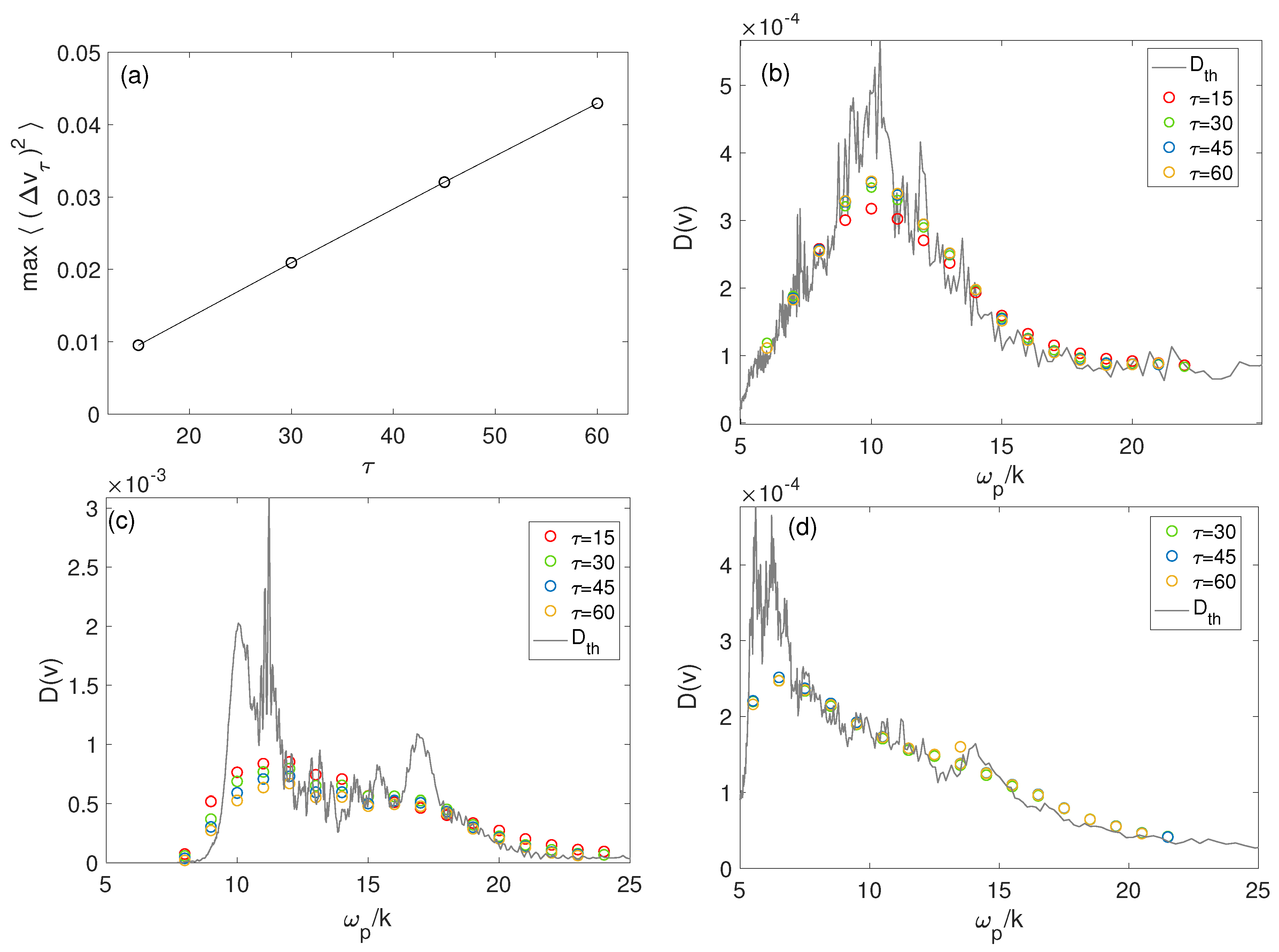
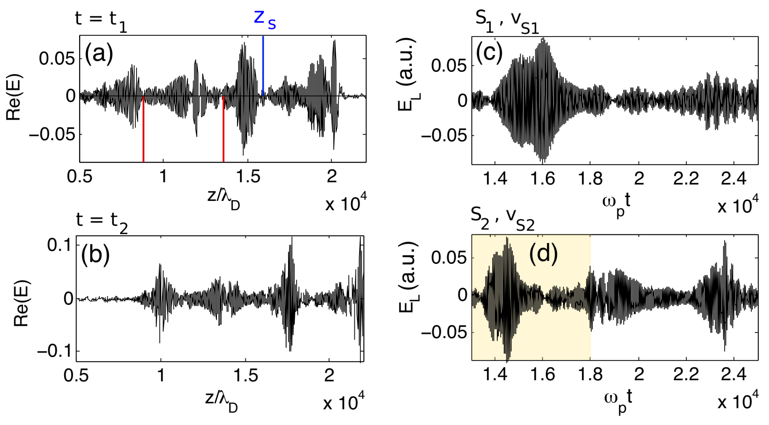
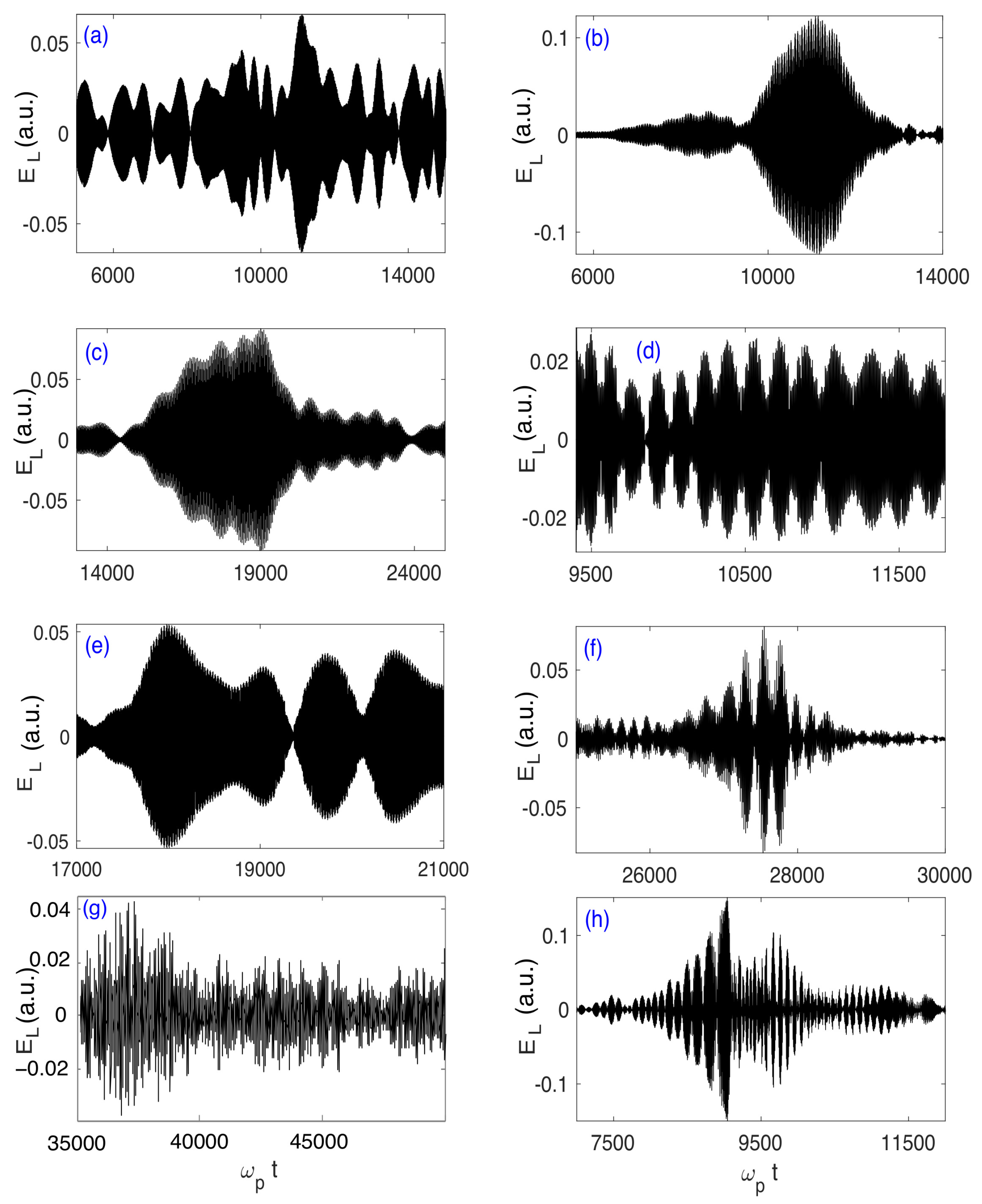
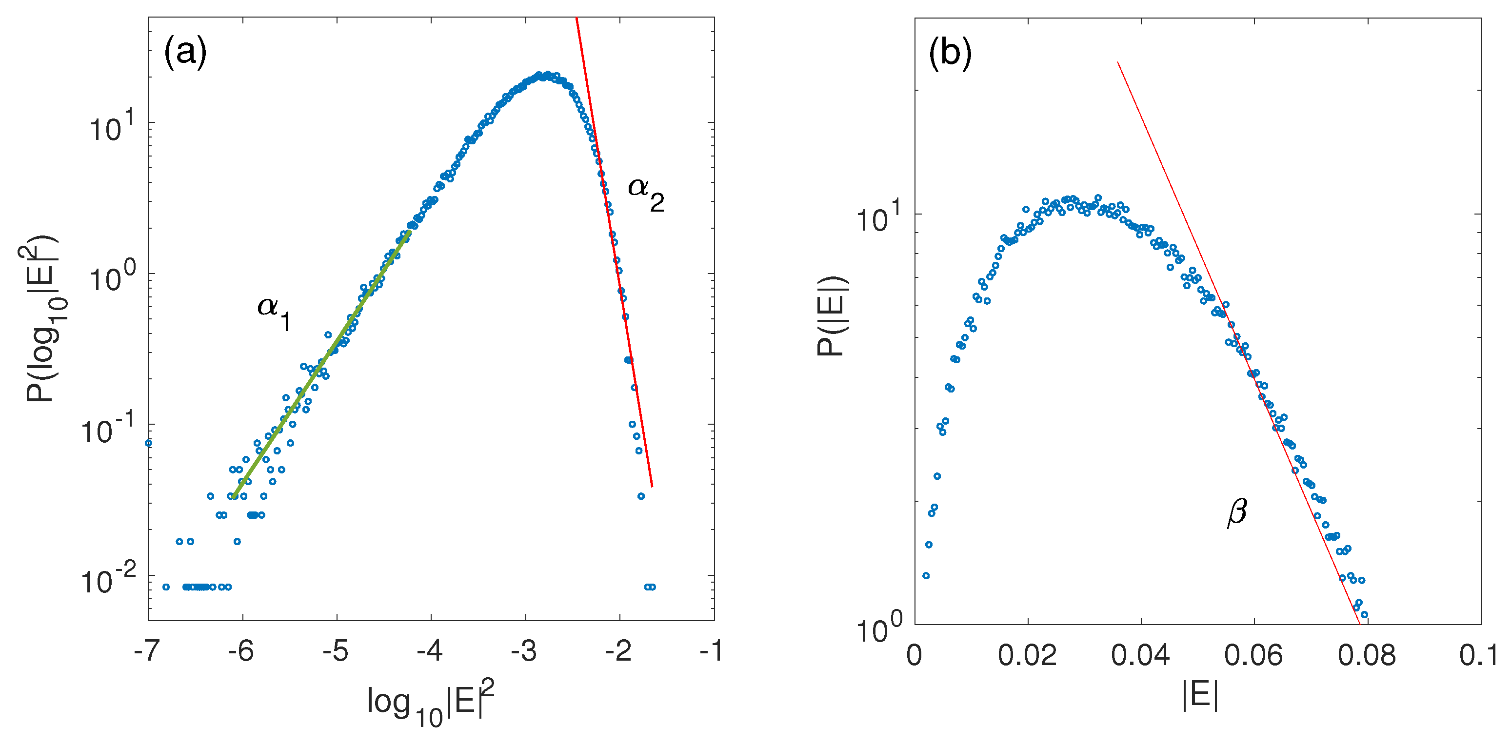
4. Conclusions

Solar radio bursts are among the strongest electromagnetic emissions in the Solar System. They are related to the existence of accelerated electron beams generated in the solar atmosphere and emitting Langmuir wave turbulence, which in turn produces electromagnetic radiation through a chain of successive mechanisms where the interactions between waves, free particles and solar wind plasmas play major roles. The solar corona and wind are turbulent and inhomogeneous plasmas involving random fluctuations of their density, velocity and ambient magnetic field.
The mechanisms governing the chain of interconnected processes forming the solar radio bursts remain to date unsolved, despite considerable advances during the last 50 years. In particular, this review presents the state of art, including some relevant results obtained by the authors, in what concerns the impact of the background plasma density fluctuations on the small-scale processes at work in the physics of solar bursts, as the dynamics of the beams, the generation of the Langmuir wave turbulence, the electron acceleration and diffusion mechanisms, the wave-wave interactions and wave decay phenomena involving Langmuir and low frequency waves, the wave transformations on the inhomogeneities (scattering, diffusion, reflection, refraction, tunneling, etc.), the modulations shaping the Langmuir waveforms, and the statistical properties of the wavefieds’ distributions.
The complexity induced by the presence of density irregularities in the solar plasmas requires to find new theoretical and numerical approaches for studying microprocesses in actual physical conditions and elucidating the key questions concerning solar bursts. Therefore, forthcoming work by the authors will be focused on the thorough study of the small-scale mechanisms at work in coronal and solar wind plasmas, in the frame of a new 2D modelling of wave turbulence in inhomogeneous plasmas including various beams’ descriptions [38]. Such investigations will be aimed at explaining additional processes, as finite magnetization effects, microinstabilities in the presence of moderate magnetic fields, mechanisms of electromagnetic radio emissions, strong turbulence phenomena, etc. These studies will be accompanied by comparisons of the simulations’ results with observations by various satellites, among which the international missions Parker Solar Probe/NASA [168] and Solar Orbiter/ESA [169].

Author Contributions

Conceptualization, C.K. and A.S.V.; methodology, C.K. and A.S.V.; software, C.K. and A.S.V.; validation, C.K. and A.S.V.; formal analysis, C.K. and A.S.V.; investigation, C.K. and A.S.V.; resources, C.K.; data curation, C.K.; writing—original draft preparation, C.K.; writing—review and editing, C.K., A.S.V. and G.G.; visualization, C.K., A.S.V. and G.G.; supervision, C.K.; project administration, C.K.; funding acquisition, C.K.

Funding

This work was granted access to the HPC resources of IDRIS under the allocation 2013-i2013057017 made by GENCI. This work has been done within the LABEX Plas@par project, and received financial state aid managed by the Agence Nationale de la Recherche, as part of the programme "Investissements d’avenir" under the reference ANR-11-IDEX-0004-02. The work was carried out with the financial support of the Russian Foundation for Basic Research, project 16-52-16010-NTSNILa.

Acknowledgments

C.K. acknowledges the “Programme National Soleil Terre” (PNST) and the Centre National d’Etudes Spatiales (CNES, France).

Conflicts of Interest

The authors declare no conflict of interest. The funders had no role in the design of the study; in the collection, analyses, or interpretation of data; in the writing of the manuscript, or in the decision to publish the results.

Abbreviations

The following abbreviations are used in this manuscript:
PICParticle-In-Cell
PDF(s)Probability distribution function(s)

References

  1. Smith, D.F.; Sime, D. Origin of plasma-wave clumping in Type III solar radio burst sources. Astrophys. J. 1979, 233, 998–1004. [Google Scholar] [CrossRef]
  2. Krupar, V.; Maksimovic, M.; Kontar, E.; Zaslavsky, A.; Santolik, O.; Soucek, J.; Kruparova, O.; Eastwood, J.; Szabo, A. Interplanetary Type III Bursts and Electron Density Fluctuations in the Solar Wind. Astrophys. J. 2018, 857, 82. [Google Scholar] [CrossRef]
  3. Chen, X.; Kontar, E.P.; Yu, S.; Yan, Y.; Huang, J.; Tan, B. Fine structures of solar radio Type III bursts and their possible relationship with coronal density turbulence. Astrophys. J. 2018, 856, 73. [Google Scholar] [CrossRef]
  4. Mugundhan, V.; Hariharan, K.; Ramesh, R. Solar Type IIIb radio bursts as tracers for electron density fluctuations in the corona. Sol. Phys. 2017, 292, 155. [Google Scholar] [CrossRef]
  5. Celnikier, L.M.; Harvey, C.C.; Jegou, R.; Moricet, P.; Kemp, M. A determination of the electron density fluctuation spectrum in the solar wind, using the ISEE propagation experiment. Astron. Astrophys. 1983, 126, 293–298. [Google Scholar]
  6. Celnikier, L.M.; Muschietti, L.; Goldman, M.V. Aspects of interplanetary plasma turbulence. Astron. Astrophys. 1987, 181, 138–154. [Google Scholar]
  7. Kellogg, P.J.; Horbury, T.S. Rapid density fluctuations in the solar wind. Ann. Geophys. 2005, 23, 3765–3773. [Google Scholar] [CrossRef]
  8. Ergun, R.E.; Malaspina, D.M.; Cairns, I.H.; Goldman, M.V.; Newman, D.L.; Robinson, P.A.; Eriksson, S.; Bougeret, J.L.; Briand, C.; Bale, S.D.; et al. Eigenmode Structure in Solar-Wind Langmuir Waves. Phys. Rev. Lett. 2008, 101, 051101. [Google Scholar] [CrossRef]
  9. Krasnoselskikh, V.; Lobzin, V.V.; Musatenko, K.; Soucek, J.; Pickett, J.S.; Cairns, I.H. Beam-plasma interaction in randomly inhomogeneous plasmas and statistical properties of small-amplitude Langmuir waves in the solar wind and electron foreshock. J. Geophys. Res. (Space Phys.) 2007, 112, A10109. [Google Scholar] [CrossRef]
  10. Krafft, C.; Volokitin, A.S.; Krasnoselskikh, V.V. Interaction of energetic particles with waves in strongly inhomogeneous solar wind plasmas. Astrophys. J. 2013, 778, 111. [Google Scholar] [CrossRef]
  11. Musher, S.L.; Rubenchik, A.M.; Zakharov, V.E. Weak Langmuir turbulence. Phys. Rep. 1995, 252, 177–274. [Google Scholar] [CrossRef]
  12. Robinson, P. Nonlinear wave collapse and strong turbulence. Rev. Mod. Phys. 1997, 69, 507. [Google Scholar] [CrossRef]
  13. Zakharov, V. Collapse and self-focusing of Langmuir waves. In Basic Plasma Physics—Handbook of Plasma Physics; North-Holland Publishing Company: Amsterdam, The Netherlands, 1983; Volume 2, pp. 81–120. [Google Scholar]
  14. Shapiro, V.; Shevchenko, V. Strong turbulence of plasma oscillations. In Basic Plasma Physics—Handbook of Plasma Physics; North-Holland Publishing Company: Amsterdam, The Netherlands, 1983; Volume 2, pp. 124–182. [Google Scholar]
  15. Davidson, R. Methods in Nonlinear Plasma Theory; Elsevier: New York, NY, USA, 2012. [Google Scholar]
  16. Galeev, A.A.; Sudan, R. Wave-wave. and wave-particle interaction. In Basic Plasma Physics—Handbook of Plasma Physics; North-Holland Publishing Company: Amsterdam, The Netherlands, 1983; Volume 1, pp. 563–570. [Google Scholar]
  17. Kundu, M.R. Solar Radio Astronomy; Interscience Publication: New York, NY, USA, 1965. [Google Scholar]
  18. Bougeret, J.L.; Caroubalos, C.; Mercier, C.; Pick, M. Sources of Type III Solar Bursts Observed at 169 MHz with the Nançay Radioheliograph. Astron. Astrophys. 1970, 6, 406. [Google Scholar]
  19. Lin, R. Non-relativistic solar electrons. Space Sci. Rev. 1974, 16, 189–256. [Google Scholar] [CrossRef]
  20. Fitzenreiter, R.; Evans, L.; Lin, R. Quantitative comparisons of Type III radio burst intensity and fast electron flux at 1 AU. Sol. Phys. 1976, 46, 437–446. [Google Scholar] [CrossRef]
  21. Gurnett, D.; Anderson, R. Electron Plasma Oscillations Associated with Type III Radio Bursts. Science 1976, 194, 1159–1162. [Google Scholar] [CrossRef] [PubMed]
  22. Gurnett, D.A.; Anderson, R.R. Plasma wave electric fields in the solar wind—Initial results from HELIOS 1. J. Geophys. Res. (Space Phys.) 1977, 82, 632–650. [Google Scholar] [CrossRef]
  23. Steinberg, J.; Hoang, S.; Lecacheux, A.; Aubier, M.; Dulk, G. Type III radio bursts in the interplanetary medium-The role of propagation. Astron. Astrophys. 1984, 140, 39–48. [Google Scholar]
  24. Suzuki, S.; Dulk, G. Bursts of Type III and Type V. In Solar Radiophysics: Studies of Emission from the Sun at Metre Wavelengths; Cambridge University Press: Cambridge, UK, 1985; pp. 289–332. [Google Scholar]
  25. Gurnett, D.A.; Frank, L.A. Electron plasma oscillations associated with Type III radio emissions and solar electrons. Sol. Phys. 1975, 45, 477–493. [Google Scholar] [CrossRef]
  26. Lin, R.; Levedahl, W.; Lotko, W.; Gurnett, D.; Scarf, F. Evidence for nonlinear wave-wave interaction in solar Type III radio bursts. Astrophys. J. 1986, 308, 954–965. [Google Scholar] [CrossRef]
  27. Reiner, M.; Stone, R.; Fainberg, J. Detection of fundamental and harmonic Type III radio emission and the associated Langmuir waves at the source region. Astrophys. J. 1992, 394, 340–350. [Google Scholar] [CrossRef]
  28. Benz, A.O.; Brajša, R.; Magdalenić, J. Are there radio-quiet solar flares? Sol. Phys. 2007, 240, 263–270. [Google Scholar] [CrossRef]
  29. Reid, H.A.S.; Ratcliffe, H. A review of solar Type III radio bursts. Res. Astr. Astrophys. 2014, 14, 773. [Google Scholar] [CrossRef]
  30. Lin, R.P.; Potter, D.W.; Gurnett, D.A.; Scarf, F.L. Energetic electrons and plasma waves associated with a solar type III radio burst. Astrophys. J. 1981, 251, 364–373. [Google Scholar] [CrossRef]
  31. Gurnett, D.A.; Kurth, W.S.; Shaw, R.R.; Roux, A.; Gendrin, R.; Kennel, C.F.; Scarf, F.L.; Shawhan, S.D. The Galileo plasma wave investigation. Space Sci. Rev. 1992, 60, 341–355. [Google Scholar] [CrossRef]
  32. Ergun, R.E.; Larson, D.; Lin, R.P.; McFadden, J.P.; Carlson, C.W.; Anderson, K.A.; Muschietti, L.; McCarthy, M.; Parks, G.K.; Reme, H.; et al. Wind Spacecraft Observations of Solar Impulsive Electron Events Associated with Solar Type III Radio Bursts. Astrophys. J. 1998, 503, 435–445. [Google Scholar] [CrossRef]
  33. Mangeney, A.; Salem, C.; Lacombe, C.; Bougeret, J.L.; Perche, C.; Manning, R.; Kellogg, P.J.; Goetz, K.; Monson, S.J.; Bosqued, J.M. WIND observations of coherent electrostatic waves in the solar wind. Ann. Geophys. 1999, 17, 307–320. [Google Scholar] [CrossRef]
  34. Kellogg, P.J.; Goetz, K.; Monson, S.J.; Bale, S.D.; Reiner, M.J.; Maksimovic, M. Plasma wave measurements with STEREO S/WAVES: Calibration, potential model, and preliminary results. J. Geophys. Res. (Space Phys.) 2009, 114, A02107. [Google Scholar] [CrossRef]
  35. Hess, S.L.G.; Malaspina, D.M.; Ergun, R.E. Size and amplitude of Langmuir waves in the solar wind. J. Geophys. Res. (Space Phys.) 2011, 116, A07104. [Google Scholar] [CrossRef]
  36. Briand, C. Plasma waves above the ion cyclotron frequency in the solar wind: A review on observations. Nonlinear Proc. Geophys. 2009, 16, 319–329. [Google Scholar] [CrossRef]
  37. Ginzburg, V.; Zhelezniakov, V. On the possible mechanisms of sporadic solar radio emission (radiation in an isotropic plasma). Astron. Zhurnal 1958, 35, 694. [Google Scholar]
  38. Volokitin, A.; Krafft, C. Electromagnetic Wave Emissions from a Turbulent Plasma with Density Fluctuations. Astrophys. J. 2018, 868, 104. [Google Scholar] [CrossRef]
  39. Kellogg, P.J. Langmuir waves associated with collisionless shocks: A review. Planet. Space Sci. 2003, 51, 681–691. [Google Scholar] [CrossRef]
  40. Brain, D. The bow shocks and upstream waves of Venus and Mars. Adv. Space Res. 2004, 33, 1913–1919. [Google Scholar] [CrossRef]
  41. Soucek, J.; Santolik, O.; de Wit, T.D.; Pickett, J.S. Cluster multispacecraft measurement of spatial scales of foreshock Langmuir waves. J. Geophys. Res. (Space Phys.) 2009, 114, A02213. [Google Scholar] [CrossRef]
  42. Gurnett, D.; Hospodarsky, G.; Kurth, W.; Williams, D.; Bolton, S. Fine Structure of Langmuir Waves Produced by a Solar Electron Event. J. Geophys. Res. (Space Phys.) 1993, 98, 5631–5637. [Google Scholar] [CrossRef]
  43. Kojima, H.; Furuya, H.; Usui, H.; Matsumoto, H. Modulated electron plasma waves observed in the tail lobe: Geotail waveform observations. Geophys. Res. Lett. 1997, 24, 3049–3052. [Google Scholar] [CrossRef]
  44. Bonnell, J.; Kintner, P.; Wahlund, J.E.; Holtet, J.A. Modulated Langmuir waves: Observations from Freja and SCIFER. J. Geophys. Res. (Space Phys.) 1997, 102, 17233–17240. [Google Scholar] [CrossRef]
  45. Kellogg, P.; Goetz, K.; Monson, S.; Bale, S. A seach for Langmuir solitons in the Earth’s foreshock. J. Geophys. Res. (Space Phys.) 1999, 104, 6751–6757. [Google Scholar] [CrossRef]
  46. Souček, J.; Krasnoselskikh, V.; de Wit, T.D.; Pickett, J.; Kletzing, C. Nonlinear decay of foreshock Langmuir waves in the presence of plasma inhomogeneities: Theory and Cluster observations. J. Geophys. Res. (Space Phys.) 2005, 110, A08102. [Google Scholar] [CrossRef]
  47. Vedenov, A.A. Theory of Turbulent Plasma; London Iliffe Book Ltd.: London, UK, 1968. [Google Scholar]
  48. Magelssen, G.; Smith, D. Nonrelativistic electron stream propagation in the solar atmosphere and Type III radio bursts. Sol. Phys. 1977, 55, 211–240. [Google Scholar] [CrossRef]
  49. Grognard, R.J. Numerical simulation of the weak turbulence excited by a beam of electrons in the interplanetary plasma. Sol. Phys. 1982, 81, 173–180. [Google Scholar] [CrossRef]
  50. Kontar, E. Dynamics of electron beams in the solar corona plasma with density fluctuations. Astron. Astrophys. 2001, 375, 629–637. [Google Scholar] [CrossRef]
  51. Ziebell, L.F.; Yoon, P.H.; Pavan, J.; Gaelzer, R. Nonlinear evolution of beam-plasma instability in inhomogeneous medium. Astrophys. J. 2011, 727, 16. [Google Scholar] [CrossRef]
  52. Pavan, J.; Ziebell, L.; Gaelzer, R.; Yoon, P. Two-dimensional nonlinear dynamics of bidirectional beam-plasma instability. J. Geophys. Res. (Space Phys.) 2009, 114, 106–117. [Google Scholar] [CrossRef]
  53. Ryutov, D. Quasilinear relaxation of an electron beam in an inhomogeneous plasma. Sov. Phys. JETP 1970, 30, 131–137. [Google Scholar]
  54. Escande, D.; De Genouillac, G. Electron burst relaxation in a fluctuating plasma-Formal dynamical model. Astron. Astrophys. 1978, 68, 405–413. [Google Scholar]
  55. Nishikawa, K.; Ryutov, D. Relaxation of relativistic electron beam in a plasma with random density inhomogeneities. J. Phys. Soc. Jpn. 1976, 41, 1757–1765. [Google Scholar] [CrossRef]
  56. Li, B.; Willes, A.J.; Robinson, P.A.; Cairns, I.H. Dynamics of beam-driven Langmuir and ion-acoustic waves including electrostatic decay. Phys. Plasmas 2003, 10, 2748–2762. [Google Scholar] [CrossRef]
  57. Kontar, E.; Pécseli, H. Nonlinear development of electron-beam-driven weak turbulence in an inhomogeneous plasma. Phys. Rev. E 2002, 65, 066408. [Google Scholar] [CrossRef]
  58. Kadomtsev, B.B. Plasma Turbulence; Academic Press: London, UK; New York, NY, USA, 1965. [Google Scholar]
  59. Henri, P.; Califano, F.; Briand, C.; Mangeney, A. Vlasov-Poisson simulations of electrostatic parametric instability for localized Langmuir wave packets in the solar wind. J. Geophys. Res. (Space Phys.) 2010, 115, A06106. [Google Scholar] [CrossRef]
  60. Umeda, T.; Ito, T. Vlasov simulation of Langmuir decay instability. Phys. Plasmas 2008, 15, 084503. [Google Scholar] [CrossRef]
  61. Huang, Y.; Huang, G.L. Solar Type III bursts and the generation of backward Langmuir wave. Chin. Astr. Astrophys. 2008, 32, 178–185. [Google Scholar] [CrossRef]
  62. Thurgood, J.O.; Tsiklauri, D. Particle-in-cell simulations of the relaxation of electron beams in inhomogeneous solar wind plasmas. J. Plasma Phys. 2016, 82, 24. [Google Scholar] [CrossRef]
  63. Voshchepynets, A.; Krasnoselskikh, V. Probabilistic model of beam-plasma interaction in randomly inhomogeneous solar wind. J. Geophys. Res. (Space Phys.) 2015, 120, 10139–10158. [Google Scholar] [CrossRef]
  64. Krafft, C.; Volokitin, A.; Krasnoselskikh, V.; de Wit, T.D. Waveforms of Langmuir turbulence in inhomogeneous solar wind plasmas. J. Geophys. Res. (Space Phys.) 2014, 119, 9369–9382. [Google Scholar] [CrossRef]
  65. Volokitin, A.; Krasnoselskikh, V.; Krafft, C.; Kuznetsov, E. Modelling of the beam-plasma interaction in a strongly inhomogeneous plasma. AIP Conf. Proc. 2013, 1539, 78–81. [Google Scholar]
  66. Krafft, C.; Volokitin, A. Hamiltonian models for resonant wave-particle interaction processes in magnetized and inhomogeneous plasmas. Eur. Phys. J. D 2014, 68, 370. [Google Scholar] [CrossRef]
  67. Krafft, C.; Volokitin, A. Electron acceleration by Langmuir waves produced by a decay cascade. Astrophys. J. 2016, 821, 99. [Google Scholar] [CrossRef]
  68. Volokitin, A.; Krafft, C. Diffusion of energetic electrons in turbulent plasmas of the solar wind. Astrophys. J. 2016, 833, 166. [Google Scholar] [CrossRef]
  69. Krafft, C.; Volokitin, A. Acceleration of energetic electrons by waves in inhomogeneous solar wind plasmas. J. Plasma Phys. 2017, 83, 705830201. [Google Scholar] [CrossRef]
  70. Volokitin, A.; Krafft, C. Velocity diffusion of energetic electrons in the solar wind. AIP Conf. Proc. 2016, 1720, 070007. [Google Scholar]
  71. Krafft, C.; Volokitin, A. Langmuir turbulence driven by beams in solar wind plasmas with long wavelength density fluctuations. AIP Conf. Proc. 2016, 1720, 040008. [Google Scholar]
  72. Krafft, C.; Volokitin, A. Langmuir wave decay in turbulent inhomogeneous solar wind plasmas. AIP Conf. Proc. 2016, 1720, 040009. [Google Scholar]
  73. Voshchepynets, A.; Volokitin, A.; Krasnoselskikh, V.; Krafft, C. Statistics of electric fields’ amplitudes in Langmuir turbulence: A numerical simulation study. J. Geophys. Res. (Space Phys.) 2017, 122, 3915–3934. [Google Scholar] [CrossRef]
  74. Krafft, C.; Volokitin, A.S.; Krasnoselskikh, V.V. Langmuir Wave Decay in Inhomogeneous Solar Wind Plasmas: Simulation Results. Astrophys. J. 2015, 809, 176. [Google Scholar] [CrossRef]
  75. Krafft, C.; Volokitin, A. Whistler envelope solitons. I. Dynamics in inhomogeneous plasmas. Phys. Plasmas 2018, 25, 102301. [Google Scholar] [CrossRef]
  76. Krafft, C.; Volokitin, A. Whistler envelope solitons. II. Interaction with non-relativistic electron beams in plasmas with density inhomogeneities. Phys. Plasmas 2018, 25, 102302. [Google Scholar] [CrossRef]
  77. Volokitin, A.; Krafft, C. Velocity diffusion in plasma waves excited by electron beams: A numerical experiment. Plasma Phys. Control. Fusion 2012, 54, 085002. [Google Scholar] [CrossRef]
  78. Zakharov, V.E. Collapse of Langmuir waves. Sov. Phys. JETP 1972, 35, 908–914. [Google Scholar]
  79. Hockney, R.W.; Eastwood, J.W. Computer Simulation Using Particles; Taylor & Francis, Inc.: Bristol, UK, 1988. [Google Scholar]
  80. O’Neil, T.; Winfrey, J.; Malmberg, J. Nonlinear interaction of a small cold beam and a plasma. Phys. Fluids 1971, 14, 1204–1212. [Google Scholar] [CrossRef]
  81. Volokitin, A.; Krafft, C. Interaction of suprathermal electron fluxes with lower hybrid waves. Phys. Plasmas 2004, 11, 3165–3176. [Google Scholar] [CrossRef]
  82. Zaslavsky, A.; Krafft, C.; Volokitin, A. Stochastic Processes of Particle Trapping and Detrapping by a Wave in a Magnetized Plasma. Phys. Rev. E 2006, 73, 016406. [Google Scholar] [CrossRef]
  83. Krafft, C.; Volokitin, A.; Zaslavsky, A. Saturation of the fan instability: Nonlinear merging of resonances. Phys. Plasmas 2005, 12, 112309. [Google Scholar] [CrossRef]
  84. Krafft, C.; Volokitin, A. Stabilization of the fan instability: Electron flux relaxation. Phys. Plasmas 2006, 13, 122301. [Google Scholar] [CrossRef]
  85. Zaslavsky, A.; Krafft, C.; Volokitin, A. Loss-Cone Instability: Wave Saturation by Particle Trapping. Phys. Plasmas 2007, 14, 122302. [Google Scholar] [CrossRef]
  86. Krafft, C.; Volokitin, A. Nonlinear fan instability of electromagnetic waves. Phys. Plasmas 2010, 17, 102303. [Google Scholar] [CrossRef]
  87. Valentini, F.; Vecchio, A.; Donato, S.; Carbone, V.; Briand, C.; Bougeret, J.; Veltri, P. The nonlinear and nonlocal link between macroscopic Alfvénic and microscopic electrostatic scales in the solar wind. Astrophys. J. 2014, 788, L16. [Google Scholar] [CrossRef]
  88. Karlickỳ, M.; Kontar, E. Electron acceleration during three-dimensional relaxation of an electron beam-return current plasma system in a magnetic field. Astron. Astrophys. 2012, 544, A148. [Google Scholar] [CrossRef]
  89. Reid, H.A.; Kontar, E.P. Evolution of the solar flare energetic electrons in the inhomogeneous inner heliosphere. Sol. Phys. 2013, 285, 217–232. [Google Scholar] [CrossRef]
  90. Vedenov, A.; Velikhov, E.; Sagdeev, R. Nonlinear oscillations of rarified plasma. Nucl. Fusion 1961, 1, 82. [Google Scholar] [CrossRef]
  91. Sturrock, P.A. Type III solar radio bursts. NASA Spec. Publ. 1964, 50, 357. [Google Scholar]
  92. Vedenov, A.; Gordeev, A.; Rudakov, L. Oscillations and instability of a weakly turbulent plasma. Plasma Phys. 1967, 9, 719. [Google Scholar] [CrossRef]
  93. Zaitsev, V.; Mityakov, N.; Rapoport, V. A dynamic theory of Type III solar radio bursts. Sol. Phys. 1972, 24, 444–456. [Google Scholar] [CrossRef]
  94. Breǐzman, B.N.; Ruytov, D.D. Quasilinear Relaxation of an Electron Beam in an Inhomogeneous Bounded Plasma. J. Exp. Theor. Phys. 1970, 30, 759. [Google Scholar]
  95. Kharchenko, I.; Feinberg, Y.B.; Nikolaev, R.; Kornilov, E.; Lutsenko, E.; Pedenko, N. The interaction of an electron beam with a plasma in a magnetic field. Zhur. Tekh. Fiz. [Sov. J.] 1961, 31, 759. [Google Scholar]
  96. Nulsen, A.L.; Cairns, I.H.; Robinson, P.A. Field distributions and shapes of Langmuir wave packets observed by Ulysses in an interplanetary Type III burst source region. J. Geophys. Res. (Space Phys.) 2007, 112, A05107. [Google Scholar] [CrossRef]
  97. Malaspina, D.M.; Cairns, I.H.; Ergun, R.E. The 2fp radiation from localized Langmuir waves. J. Geophys. Res. (Space Phys.) 2010, 115, A01101. [Google Scholar] [CrossRef]
  98. Melrose, D.B.; Cairns, I.H.; Dulk, G.A. Clumpy Langmuir waves in Type III solar radio bursts. Astron. Astrophys. 1986, 163, 229–238. [Google Scholar]
  99. Melrose, D. A phase-bunching mechanism for fine structures in auroral kilometric radiation and Jovian decametric radiation. J. Geophys. Res. (Space Phys.) 1986, 91, 7970–7980. [Google Scholar] [CrossRef]
  100. Robinson, P.; Cairns, I.; Gurnett, D. Connection between ambient density fluctuations and clumpy Langmuir waves in Type III radio sources. Astrophys. J. 1992, 387, 101–104. [Google Scholar] [CrossRef]
  101. Robinson, P.A.; Willes, A.J.; Cairns, I.H. Dynamics of Langmuir and ion-sound waves in Type III solar radio sources. Astrophys. J. 1993, 408, 720–734. [Google Scholar] [CrossRef]
  102. Boshuizen, C.R.; Cairns, I.H.; Robinson, P.A. Electric field distributions for Langmuir waves in planetary foreshocks. J. Geophys. Res. (Space Phys.) 2004, 109, A08101. [Google Scholar] [CrossRef]
  103. Mel’Nik, V.; Lapshin, V.; Kontar, E. Propagation of a monoenergetic electron beam in the solar corona. Sol. Phys. 1999, 184, 353–362. [Google Scholar] [CrossRef]
  104. Li, B.; Robinson, P.A.; Cairns, I.H. Numerical Simulations of Type-III Solar Radio Bursts. Phys. Rev. Lett. 2006, 96, 145005. [Google Scholar] [CrossRef] [PubMed]
  105. Kellogg, P.J.; Goetz, K.; Lin, N.; Monson, S.J.; Balogh, A.; Forsyth, R.; Stone, R.G. Low frequency magnetic signals associated with Langmuir waves. Geophys. Res. Lett. 1992, 19, 1299–1302. [Google Scholar] [CrossRef]
  106. Thejappa, G.; MacDowall, R.J.; Bergamo, M. In situ detection of strong Langmuir turbulence processes in solar Type III radio bursts. J. Geophys. Res. (Space Phys.) 2012, 117, 8111. [Google Scholar] [CrossRef]
  107. Goldman, M.V. Strong turbulence of plasma waves. Rev. Mod. Phys. 1984, 56, 709–735. [Google Scholar] [CrossRef]
  108. Newman, D.; Winglee, R.; Robinson, P.; Glanz, J.; Goldman, M. Simulation of collapse and dissipation of Langmuir wave packet. Phys. Pluids B 1990, 2, 2600–2622. [Google Scholar] [CrossRef]
  109. Gurnett, D.A.; Maggs, J.E.; Gallagher, D.L.; Kurth, W.S.; Scarf, F.L. Parametric interaction and spatial collapse of beam-driven Langmuir waves in the solar wind. J. Geophys. Res. (Space Phys.) 1981, 86, 8833–8841. [Google Scholar] [CrossRef]
  110. Cairns, I.H.; Robinson, P.A. Theory for low-frequency modulated Langmuir wave packets. Geophys. Res. Lett. 1992, 19, 2187–2190. [Google Scholar] [CrossRef]
  111. Robinson, P.A.; Newman, D.L. Strong plasma turbulence in the Earth’s electron foreshock. J. Geophys. Res. (Space Phys.) 1991, 96, 17733–17749. [Google Scholar] [CrossRef]
  112. Hospodarsky, G.B.; Gurnett, D.A.; Kurth, W.S.; Kivelson, M.G.; Strangeway, R.J.; Bolton, S.J. Fine structure of Langmuir waves observed upstream of the bow shock at Venus. J. Geophys. Res. (Space Phys.) 1994, 99, 13363–13371. [Google Scholar] [CrossRef]
  113. Hospodarsky, G.; Gurnett, D. Beat-type Langmuir wave emissions associated with a type III solar radio bursts. Geophys. Res. Lett. 1995, 22, 1161–1164. [Google Scholar] [CrossRef]
  114. Bale, S.; Burgess, D.; Kellogg, P.; Goetz, K.; Howard, R.; Monson, S. Phase coupling in Langmuir wave packets: Possible evidence of three wave interactions in the upstream solar wind. Geophys. Res. Lett. 1996, 23, 109–112. [Google Scholar] [CrossRef]
  115. Thejappa, G.; MacDowall, R.J.; Scime, E.E.; Littleton, J.E. Evidence for electrostatic decay in the solar wind at 5.2 AU. J. Geophys. Res. (Space Phys.) 2003, 108, 1139. [Google Scholar] [CrossRef]
  116. Henri, P.; Briand, C.; Mangeney, A.; Bale, S.D.; Califano, F.; Goetz, K.; Kaiser, M. Evidence for wave coupling in Type III emissions. J. Geophys. Res. (Space Phys.) 2009, 114, A03103. [Google Scholar] [CrossRef]
  117. Graham, D.B.; Cairns, I.H.; Robinson, P.A. Langmuir "snakes" and electrostatic decay in the solar wind. Geophys. Res. Lett. 2013, 40, 1934–1939. [Google Scholar] [CrossRef]
  118. Bougeret, J.L.; Goetz, K.; GoldsteinKaiser, M.; Bale, S.; Kellogg, P.; Maksimovic, M.; Monge, N.; Monson, S.; Astier, P.; Davy, S.; et al. S/WAVES: The radio and plasma wave investigation on the STEREO Mission. Space Sci. Rev. 2008, 136, 487–529. [Google Scholar] [CrossRef]
  119. Burinskaya, T.M.; Rauch, J.L.; Mogilevskii, M.M. Spectra of Langmuir waves in a magnetized plasma with low-frequency turbulence. Plasma Phys. Rep. 2004, 30, 756–760. [Google Scholar] [CrossRef]
  120. Melrose, D. Plasma emission: A review. Sol. Phys. 1987, 111, 89–101. [Google Scholar] [CrossRef]
  121. Ziebell, L.; Gaelzer, R.; Yoon, P.H. Nonlinear development of weak beam–plasma instability. Phys. Plasmas 2001, 8, 3982–3995. [Google Scholar] [CrossRef]
  122. Gibson, S.; Newman, D.; Goldman, M. Langmuir turbulence and three-wave nonlinear dynamics. Phys. Rev. E 1995, 52, 558–571. [Google Scholar] [CrossRef]
  123. Nicholson, D.R.; Goldman, M.V. Cascade and collapse of Langmuir waves in two dimensions. Phys. Fluids 1978, 21, 1766–1776. [Google Scholar] [CrossRef]
  124. Galeev, A.; Sagdeev, R.; Sigov, U.; Shapiro, V.; Shevehenko, V. Nonlinear theory for the modulation instability of plasma waves. Sov. J. Plasma Phys. 1975, 1, 5–10. [Google Scholar]
  125. Graham, D.B.; Cairns, I.H. Electrostatic decay of Langmuir/z-mode waves in Type III solar radio bursts. J. Geophys. Res. (Space Phys.) 2013, 118, 3968–3984. [Google Scholar] [CrossRef]
  126. Kontar, E.; Ratcliffe, H.; Bian, N. Wave-particle interactions in non-uniform plasma and the interpretation of hard X-ray spectra in solar flares. Astron. Astrophys. 2012, 539, A43. [Google Scholar] [CrossRef]
  127. Pechhacker, R.; Tsiklauri, D. Three-dimensional particle-in-cell simulation of electron acceleration by Langmuir waves in an inhomogeneous plasma. Phys. Plasmas 2014, 21, 012903. [Google Scholar] [CrossRef]
  128. Vedenov, A.; Velikhov, E.; Sagdeev, R. Quasi-linear theory of plasma oscillations. Nucl. Fusion Suppl. 1962, 2, 465. [Google Scholar]
  129. Drummond, W.; Pines, D. Non-linear stability of plasma oscillation. Nucl. Fusion Suppl. 1962, 3, 1049. [Google Scholar]
  130. Theilhaber, K.; Laval, G.; Pesme, D. Numerical simulations of turbulent trapping in the weak beam–plasma instability. Phys. Fluids 1987, 30, 3129–3149. [Google Scholar] [CrossRef]
  131. Besse, N.; Elskens, Y.; Escande, D.F.; Bertrand, P. Validity of quasilinear theory: Refutations and new numerical confirmation. Plasma Phys. Control. Fusion 2011, 53, 025012. [Google Scholar] [CrossRef]
  132. Doveil, F.; Grésillon, D. Statistics of charged particles in external random longitudinal electric fields. Phys. Fluids 1982, 25, 1396–1402. [Google Scholar] [CrossRef]
  133. Cary, J.R.; Escande, D.F.; Verga, A.D. Nonquasilinear diffusion far from the chaotic threshold. Phys. Rev. Lett. 1990, 65, 3132. [Google Scholar] [CrossRef] [PubMed]
  134. Xia, H.; Ishihara, O.; Hirose, A. Non-Markovian diffusion in plasma turbulence. Phys. Fluids B Plasma Phys. 1993, 5, 2892–2904. [Google Scholar] [CrossRef]
  135. Xia, H.; Ishihara, O.; Watanabe, S. Long-time diffusion in plasma turbulence with broad uniform spectrum. Phys. Fluids B Plasma Phys. 1993, 5, 2786–2792. [Google Scholar]
  136. Helander, P.; Kjellberg, L. Simulation of nonquasilinear diffusion. Phys. Plasmas 1994, 1, 210–212. [Google Scholar] [CrossRef]
  137. Hirose, A.; Edler, K.; Bolster, E.; Ishihara, O. Electron velocity diffusion in strong turbulence. IEEE Trans. Plasma Sci. 2003, 31, 3–6. [Google Scholar] [CrossRef]
  138. Zagorodny, A.; Zasenko, V.; Weiland, J.; Holod, I. Particle diffusion in random fields: Time-nonlocal description and numerical simulations. Phys. Plasmas 2003, 10, 58–68. [Google Scholar] [CrossRef]
  139. Zasenko, V.; Zagorodny, A.; Weiland, J. Stochastic acceleration in peaked spectrum. Phys. Plasmas 2005, 12, 062311. [Google Scholar] [CrossRef]
  140. Bian, N.H.; Kontar, E.P.; Ratcliffe, H. Resonance broadening due to particle scattering and mode coupling in the quasi-linear relaxation of electron beams. J. Geophys. Res. (Space Phys.) 2014, 119, 4239–4255. [Google Scholar] [CrossRef]
  141. Gurnett, D.A.; Anderson, R.R.; Scarf, F.L.; Kurth, W.S. The heliocentric radial variation of plasma oscillations associated with Type III radio bursts. J. Geophys. Res. (Space Phys.) 1978, 83, 4147–4152. [Google Scholar] [CrossRef]
  142. Malaspina, D.M.; Cairns, I.H.; Ergun, R.E. Dependence of Langmuir wave polarization on electron beam speed in Type III solar radio bursts. Geophys. Res. Lett. 2011, 38, L13101. [Google Scholar] [CrossRef]
  143. Robinson, P.A. Clumpy Langmuir waves in Type III radio sources. Sol. Phys. 1992, 139, 147–163. [Google Scholar] [CrossRef]
  144. Kellogg, P.J. Observations Concerning the Generation and Propagation of Type III Solar Bursts. Astron. Astrophys. 1986, 169, 329–335. [Google Scholar]
  145. Malaspina, D.M.; Ergun, R.E. Observations of three-dimensional Langmuir wave structure. J. Geophys. Res. (Space Phys.) 2008, 113, A12108. [Google Scholar] [CrossRef]
  146. Zaslavsky, A.; Volokitin, A.; Krasnoselskikh, V.V.; Maksimovic, M.; Bale, S.D. Spatial localization of Langmuir waves generated from an electron beam propagating in an inhomogeneous plasma: Applications to the solar wind. J. Geophys. Res. (Space Phys.) 2010, 115, A08103. [Google Scholar] [CrossRef]
  147. Muschietti, L.; Roth, I.; Ergun, R. Interaction of Langmuir wave packets with streaming electrons: Phase-correlation aspects. Phys. Plasmas 1994, 1, 1008–1024. [Google Scholar] [CrossRef]
  148. Muschietti, L.; Roth, I.; Ergun, R.E. Kinetic localization of beam-driven Langmuir waves. J. Geophys. Res. (Space Phys.) 1995, 100, 17481–17490. [Google Scholar] [CrossRef]
  149. Nicholson, D.R.; Goldman, M.V.; Hoyng, P.; Weatherall, J.C. Nonlinear Langmuir Waves During Type III Solar Radio Bursts. Astrophys. J. 1978, 223, 605–619. [Google Scholar] [CrossRef]
  150. Astron. LOFAR. 2019. Available online: http://www.lofar.org/ (accessed on 1 March 2019).
  151. De La Noe, J.; Boischot, A. The Type III b burst. Astron. Astrophys. 1972, 20, 55. [Google Scholar]
  152. Graham, D.B.; Cairns, I.H.; Prabhakar, D.R.; Ergun, R.E.; Malaspina, D.M.; Bale, S.D.; Goetz, K.; Kellogg, P.J. Do Langmuir wave packets in the solar wind collapse? J. Geophys. Res. (Space Phys.) 2012, 117, A09107. [Google Scholar] [CrossRef]
  153. Graham, D.B.; Cairns, I.H. Constraints on the Formation and Structure of Langmuir Eigenmodes in the Solar Wind. Phys. Rev. Lett. 2013, 111, 121101. [Google Scholar] [CrossRef]
  154. Li, B.; Cairns, I.H.; Robinson, P.A.; LaBelle, J.; Kletzing, C.A. Waveform and envelope field statistics for waves with stochastically driven amplitudes. Phys. Plasmas 2010, 17, 032110. [Google Scholar] [CrossRef]
  155. Reid, H.A.; Kontar, E.P. Langmuir wave electric fields induced by electron beams in the heliosphere. Astron. Astrophys. 2017, 598, A44. [Google Scholar] [CrossRef]
  156. Bale, S.; Kellog, P.; Larson, D.; Lin, R.; Goetz, K.; Lepping, R. Bipolar electrostatic structures in the shock transition region: Evidence of electron phase space holes. Geophys. Res. Lett. 1998, 25, 2929–2932. [Google Scholar] [CrossRef]
  157. LaBelle, J.; Cairns, I.H.; Kletzing, C.A. Electric field statistics and modulation characteristics of bursty Langmuir waves observed in the cusp. J. Geophys. Res. (Space Phys.) 2010, 115, 317. [Google Scholar] [CrossRef]
  158. Cairns, I.H.; Robinson, P.A. Strong Evidence for Stochastic Growth of Langmuir-like Waves in Earth’s Foreshock. Phys. Rev. Lett. 1999, 82, 3066–3069. [Google Scholar] [CrossRef]
  159. Cairns, I.H.; Menietti, J.D. Stochastic growth of waves over Earth’s polar cap. J. Geophys. Res. (Space Phys.) 2001, 106, 29515–29529. [Google Scholar] [CrossRef]
  160. Austin, D.; Hole, M.; Robinson, P.A.; Cairns, I.H.; Dallaqua, R. Laboratory evidence for stochastic plasma-wave growth. Phys. Rev. Lett. 2007, 99, 205004. [Google Scholar] [CrossRef]
  161. Bale, S.D.; Burgess, D.; Kellogg, P.J.; Goetz, K.; Monson, S.J. On the amplitude of intense Langmuir waves in the terrestrial electron foreshock. J. Geophys. Res. (Space Phys.) 1997, 102, 11281–11286. [Google Scholar] [CrossRef]
  162. Cairns, I.H.; Robinson, P. First test of stochastic growth theory for Langmuir waves in Earth’s foreshock. Geophys. Res. Lett. 1997, 24, 369–372. [Google Scholar] [CrossRef]
  163. Pearson, K. Contributions to the mathematical theory of evolution. II. Skew variation in homogeneous material. Philos. Trans. R. Soc. A 1895, 186, 343–424. [Google Scholar] [CrossRef]
  164. Voshchepynets, A.; Krasnoselskikh, V.; Artemyev, A.; Volokitin, A. Probabilistic Model of Beam–Plasma Interaction in Randomly Inhomogeneous Plasma. Astrophys. J. 2015, 807, 38. [Google Scholar] [CrossRef]
  165. Píša, D.; Hospodarsky, G.B.; Kurth, W.S.; Santolík, O.; Souček, J.; Gurnett, D.A.; Masters, A.; Hill, M.E. Statistics of Langmuir wave amplitudes observed inside Saturn’s foreshock by the Cassini spacecraft. J. Geophys. Res. (Space Phys.) 2015, 120, 2531–2542. [Google Scholar] [CrossRef]
  166. Briand, C.; Henri, P.; Génot, V.; Lormant, N.; Dufourg, N.; Cecconi, B.; Nguyen, Q.; Goetz, K. STEREO database of interplanetary Langmuir electric waveforms. J. Geophys. Res. (Space Phys.) 2016, 121, 1062–1070. [Google Scholar] [CrossRef]
  167. Vidojević, S.; Zaslavsky, A.; Maksimović, M.; Dražić, M.; Atanacković, O. Statistical analysis of Langmuir waves associated with Type III radio bursts: I. Wind observations. Open Astron. 2011, 20, 596–599. [Google Scholar] [CrossRef]
  168. NASA. Parker Solar Probe. 2019. Available online: http://parkersolarprobe.jhuapl.edu/ (accessed on 1 March 2019).
  169. ESA. Solar Orbiter. 2019. Available online: http://sci.esa.int/solar-orbiter/ (accessed on 1 March 2019).
Figure 1. Langmuir wave packet at time ω p t = 3000 in a inhomogeneous plasma with Δ n 0.01 . (Left panel): Spatial profiles along the coordinate z / λ D of the electric field envelope Re ( E ) (blue), the density fluctuations δ n / n 0 (black) and the turbulence level E 2 × 10 (red). (Right panel): Corresponding electric field spectrum E k in logarithmic scales, as a function of the normalized wave number k λ D . No beam is present. All variables are normalized. (Reproduced by permission of the AAS [10]).
Fluids 04 00069 g001
Figure 2. Beam dynamics’ and wave packet’s evolution at three moments of time, ω p t = 2000 , 15,000 and 35,000 (from upper to lower rows). (Left panels): Spatial profiles of the electric field envelope Re | E | (blue) and of the energy density 2 E 2 (red), superposed to the density fluctuations δ n / n 0 (black). (Middle panels): Corresponding electric field spectra E k 2 in logarithmic scales. (Right panels): Corresponding electron velocity distributions f ( v ) (grey surfaces), superposed to the initial distribution (red curves). Main parameters are the following: v b / v T = 14 , Δ v b / v b = 0.08 , n b / n 0 2.5 × 10 5 , Δ n 0.001 . All variables are normalized. (Reproduced by permission of the AAS [10]).
Fluids 04 00069 g002
Figure 3. Beam dynamics’ and wave packet’s evolution at three moments of time, ω p t = 2000 , 7000 and 23,000 (from upper to lower rows). (Left panels): Spatial profiles of the electric field envelope Re E (blue) and of the energy density E 2 × 10 (red), superposed to the density fluctuations δ n / n 0 (black). (Middle panels): Corresponding electric field spectra E k 2 in logarithmic scales. (Right panels): Corresponding electron velocity distributions f ( v ) (grey surfaces), superposed to the initial distribution (red curves). Main parameters are the following : v b / v T = 14 , Δ v b / v b = 0.08 , n b / n 0 2.5 × 10 5 , Δ n 0.01 . All variables are normalized.
Fluids 04 00069 g003
Figure 4. Beam dynamics’ and wave packet’s evolution at three moments of times, ω p t = 1000 , 35,000 and 90,000 (from upper to lower rows). (Left panels): Spatial profiles of the electric field envelope Re E (blue) and of the energy density E 2 × 20 (red), superposed to the density fluctuations δ n / n 0 (black). (Middle panels): Corresponding electric field spectra E k 2 in logarithmic scales. (Right panels): Corresponding electron velocity distributions f ( v ) (grey surfaces), superposed to the initial distribution (red curves). Main parameters are the following : v b = 14 / v T , Δ v b / v b = 0.08 , n b / n 0 2.5 × 10 5 , Δ n 0.03 . All variables are normalized. (Reproduced by permission of the AAS [10]).
Fluids 04 00069 g004
Figure 5. (a) Variation with time of the wave energy density W L = k E k 2 , for different average levels of density fluctuations Δ n = 0.001 , 0.005 , 0.02 and 0.04 . (b) Corresponding variations with Δ n > Δ n s of the normalized rate of growth Ω W of the wave packets. (c,d) Variations with time of the beam velocity distributions f ( v ) for a quasi-homogeneous ( Δ n = 0.001 ) and a strongly inhomogeneous ( Δ n = 0.04 ) plasma, respectively; the initial distributions are labeled in red; in (c), the part presented in blue corresponds to a process of beam acceleration due to wave decay and not to density homogeneities. Main parameters are the following: v b / v T = 14 , Δ v b / v b = 0.08 , n b / n 0 2.5 × 10 5 . All variables are normalized.
Fluids 04 00069 g005
Figure 6. (a) Wave energy spectra E k 2 (in logarithmic scales) at asymptotic times, as a function of the phase velocities v = ω k / k 3 v T above the thermal range, for Δ n 0.001 Δ n s (green, at ω p t = 35,000) and Δ n 0.04 > Δ n s (blue, at ω p t = 70,000). (b) Corresponding electron velocity distributions f ( v ) (in logarithmic scales), superposed to the initial distribution (red), for Δ n 0.001 at ω p t = 35,000 (green) and Δ n 0.04 at ω p t = 70,000 (blue). Main parameters are the following: v b / v T = 14 , Δ v b / v b = 0.08 , n b / n 0 2.5 × 10 5 . All variables are normalized.
Fluids 04 00069 g006
Figure 7. (a) (Left panels): profiles along the coordinate z / λ D of the normalized wave energy density | E | 2 at times ω p t = 22,000 and ω p t = 35,000. (Right panels): corresponding profiles of the density fluctuations δ n / n 0 ; short-scale oscillations δ n s / n 0 are growing with time. The main parameters are the following: n b / n 0 = 5 × 10 5 , v b / v T = 14 , Δ n = 0.001 . (b) (Left panels): profiles of the normalized wave energy density | E | 2 at times ω p t = 30,000 and ω p t = 52,000. (Right panels): corresponding profiles of the density fluctuations δ n / n 0 ; the localized regions of growth of the short-scale oscillations δ n s / n 0 are colorized. The main parameters are the following: n b / n 0 = 2 × 10 5 , v b / v T = 18 , Δ n = 0.01 . All variables are normalized.
Fluids 04 00069 g007
Figure 8. Quasi-homogeneous plasma. (a) Space-time variations of the Langmuir energy density | E | 2 . (b) Space-time variations of the short-wavelength ion acoustic waves | δ n s | / n 0 . (c) Time variation of the Langmuir energy spectrum | E k | 2 . (d) Time variations of the energy densities W L and W S of the Langmuir (blue) and ion acoustic (red) waves. Main parameters are the following: Δ n = 0.001 , v b / v T = 14 , n b / n 0 = 5 × 10 5 , c s / v T = 0.045 , γ e , γ i = 0 . Examples of Langmuir and ion acoustic wave packets participating to decay processes are indicated by arrows in (a,b). All variables are normalized.
Fluids 04 00069 g008
Figure 9. Inhomogeneous plasma. (a) Space-time variations of the Langmuir energy density | E | 2 . (b) Langmuir wave energy spectrum at ω p t = 89,000. (c) Ion acoustic wave energy spectrum S k at ω p t = 89,000. (d) Time variations of the energy densities W L and W S of the Langmuir (blue) and ion acoustic (red) waves. Main parameters are the following: Δ n = 0.01 , v b / v T = 18 , n b / n 0 = 5 × 10 5 , c s / v T = 0.045 , γ e , γ i 0 (wave damping is included). Langmuir and ion acoustic wave packets participating to decay processes are indicated by arrows in (a). All variables are normalized.
Fluids 04 00069 g009
Figure 10. Cascades of wave decay. Space and time variations of | E | 2 (a) and of the corresponding short-scale density fluctuations | δ n s | / n 0 (b), in the area [ 5000 , 8000 ] λ D of the simulation box. (c) Space and time variations of | E | 2 in the area [ 5000 , 10 , 000 ] λ D of the simulation box. The main parameters are the following: (a,b) n b / n 0 = 5 × 10 5 , v b / v T = 14 , Δ n = 0.02 > Δ n s ; (c) n b / n 0 = 5 × 10 5 , v b / v T = 16 , Δ n = 0 . 01 > Δ n s . Langmuir and ion acoustic wave packets participating to decay processes are indicated by arrows. All variables are normalized.
Fluids 04 00069 g010
Figure 11. Langmuir waveforms (registered electric fields E L as a function of time) observed by a virtual satellite moving at the velocity v S = 0 . 1 v T and starting at time ω p t = 50,000 when (a) it crosses a plasma region where wave decay occurs, (b) it crosses no region with decay. (c) Langmuir waveform observed by a virtual satellite moving with v S = 0.15 v T , starting at ω p t = 40,000 and crossing a plasma region with wave decay. Main parameters are the following: (a,b) Δ n = 0.02 , (c) Δ n = 0.03 . Regions showing specific modulations due to wave decay are colorized. All variables are normalized.
Fluids 04 00069 g011
Figure 12. Time variations of different characteristics of the population of accelerated particles, for Δ n = 0.001 (green), 0.005 (red), 0.02 (yellow), and 0.04 (blue). (a): Langmuir wave energy density W L as a function of time. (b): Beam kinetic energy K t as a function of time. (c): Kinetic energy K a c carried by the accelerated electrons, as a function of time. (d): Density n a c of the accelerated electrons, as a function of time. (e): Fraction W L , a c of the energy density W L carried by the Langmuir waves with phase velocity v φ > v a c , as a function of time. (f): Ratio W L , a c / W L as a function of time. Main parameters are the following: v b / v T = 14 , n b / n 0 = 5 × 10 5 . All variables are normalized (see the text).
Fluids 04 00069 g012
Figure 13. Variation with Δ n , at asymptotic time, of the density n (blue circles) and the kinetic energy K (green stars) of the accelerated electrons, as well as of the kinetic beam energy K t , (red crosses). The density and the energy are normalized by the initial beam density and kinetic energy, respectively.
Fluids 04 00069 g013
Figure 14. (a): Variation as a function of Δ n of the maximum W m of the Langmuir wave energy density W L (blue), as well as of the saturated energy densities of all the Langmuir waves, W ¯ (red), and of the Langmuir waves with phase velocities v φ > v a c , W ¯ a c (green). (b): Thermal velocity Δ V gained by the accelerated tail with respect to the initial beam velocity distribution, as a function of Δ n . (c): Variation of W ¯ (red) and W ¯ a c (green) with Δ V . All variables are normalized ( Δ V is normalized by v T ).
Fluids 04 00069 g014
Figure 15. Velocity distribution f ( v ) of the beam for a quasi-homogeneous plasma with Δ n = 0 . 001 , at (i) ω p t = 0 (truncated, red), (ii) ω p t = 47,500 (green) and (iii) ω p t 170,000 (blue). Points (circles) provided by the simulations are fitted by Gaussian distributions (solid lines) for the beam accelerated tail, taking into account only velocities v larger than the initial beam velocity v b . The points excluded from these fits and representing the decelerated plateau are labeled by crosses. Velocities are normalized by the electron thermal velocity v T . (Reproduced with permission from [69]).
Fluids 04 00069 g015
Figure 16. (a): Time variation of the kinetic energy density K a c of the accelerated electrons (solid line), of the kinetic energy density K < a c of the accelerated electrons with velocity v < v a c = 15 . 7 (dashed-dotted line), and of the absolute value of the energy density lost by the beam, K l = 1 ( K a c + K < a c ) (dashed line). (b): Time variation of the corresponding electron densities n a c and n < a c . Main parameters are: n b / n 0 = 5 × 10 5 , v b / v T = 14 and Δ n 0 . 01 . The energies and densities are normalized by the initial beam kinetic energy and density, respectively. (Reproduced by permission of the AAS [67]).
Fluids 04 00069 g016
Figure 17. (a,b) Inhomogeneous plasma with Δ n = 0 . 01 : time variation of (a) the velocity v ( t ) and (b) the velocity variations δ v τ ( t ) = v t v t τ of a typical test particle. (c,d) Homogeneous plasma: time variation of (c) the velocity v ( t ) and (d) the velocity variations δ v τ ( t ) = v t v t τ of a typical test particle. Main parameters are: v b / v T = 12 , n b / n 0 = 10 4 , τ = 20 . Particle velocities are normalized by the plasma thermal velocity v T .
Fluids 04 00069 g017
Figure 18. Inhomogeneous plasma with Δ n = 0 . 01 . (a): Typical probability distribution functions P ( δ v τ ) , in logarithmic scale, for different values of τ = 15 (black), 30 (red), 45 (green), and 60 (blue). Insert: Variation of ( δ v τ ) 2 with τ . (b): Typical probability distribution function P ( δ v τ ) , in logarithmic scale, for τ = 30 and another time interval Δ T than (a). The calculated probabilities are shown by circles whereas the interpolation functions at moderate and large δ v τ are the sum of two Gaussians (blue curve) and the sum of a Gaussian and a power function (green curves). Homogeneous plasma ( Δ n = 0 ). (c) Homogeneous plasma: Typical probability distribution function P h ( δ v τ ) , in logarithmic scale, for τ = 20 . Insert: Variation of ( δ v τ ) 2 with τ . The calculated probabilities are shown by circles whereas the interpolation functions at moderate and large δ v τ are Gaussian (blue curves) and exponential functions (green curves). Main parameters are: v b / v T = 18 , n b / n 0 = 5 × 10 5 . The velocity increments δ v τ are normalized by the plasma thermal velocity v T .
Fluids 04 00069 g018
Figure 19. Diffusion in inhomogeneous plasmas. (a,b): Dependence of the maximum of ( Δ v τ ) 2 on τ , and calculated diffusion coefficients D ( v ) = ( Δ v τ ) 2 / 2 τ for Δ n = 0 . 01 and τ = 15 , 30, 45, and 60 (red, green, blue and yellow circles, respectively), as a function of the wave phase velocity v = ω k / k ω p / k , superposed to the diffusion coefficient D t h ( v ) derived from the quasilinear theory (grey lines). (c,d): Diffusion coefficients D ( v ) = ( Δ v τ ) 2 / 2 τ and D t h ( v ) as a function of the wave phase velocity ω p / k ; (c) Δ T = [ 35 , 000 , 43 , 000 ] , τ = 15 , 30 , 45 , 60 and Δ n = 0 . 01 ; (d) Δ T = [ 90 , 000 , 145 , 000 ] , τ = 30 , 45 , 60 and Δ n = 0 . 04 . Main parameters are: v b / v T = 14 , n b / n 0 = 5 × 10 5 . Δ T and τ are normalized by ω p ; the phase velocity ω p / k is normalized by v T .
Fluids 04 00069 g019
Figure 20. (a,b) Spatial profiles along the coordinate z / λ D of the electric field envelope Re ( E ) at times t 1 = 13,000 ω p 1 and t 2 = 25 , 000 ω p 1 . (c,d) Corresponding waveforms E L ( t ) observed by two virtual satellites S 1 and S 2 starting at the position z S at times t 1 and t 2 , and moving relatively to the solar wind with the velocities v S 1 and v S 2 , respectively; the position z S is indicated by an upward vertical line in (a), whereas the final positions of the satellites are marked by downward vertical lines; E L is normalized as the field E, and t is the time in units of ω p 1 . Main parameters are the following: n b / n 0 = 10 5 , v b / v T = 18 , Δ n 0 . 01 .
Fluids 04 00069 g020
Figure 21. (ah) Langmuir waveforms E L ( t ) (in arbitrary units) recorded by virtual satellites moving in random fluctuating inhomogeneous solar wind plasmas, calculated owing to numerical simulations. These exemples summarize all the main types of waveforms actually observed in the solar wind. Main parameters are the following: (a) v S / v T = 0 . 6 , Δ n = 0 . 001 . (b) v S / v T = 0 . 1 , Δ n = 0 . 01 . (c) v S / v T = 0 . 01 , Δ n = 0 . 01 . (d) v S / v T = 0 . 6 , Δ n = 0 . 01 . (e) v S / v T = 0 . 1 , Δ n = 0 . 001 . (f) v S / v T = 0 . 6 , Δ n = 0 . 01 . (g) v S / v T = 0 . 15 , Δ n = 0 . 04 . (h) v S / v T = 0 . 2 , Δ n = 0 . 02 .
Fluids 04 00069 g021
Figure 22. PDFs of the electric fields’ amplitudes averaged over the time interval Δ T . (a) Distribution of log 10 | E | 2 , with linear fits of slopes α 1 2.3 and α 2 9.7 . (b) Distribution of | E | , with a linear fit at large | E | of slope β 5.8 . Main parameters are : Δ n 0 . 001 , n b / n 0 = 5 × 10 5 , Δ T = [ 50 , 000 , 60 , 000 ] . Field and time variables are normalized, but not the PDFs. (Reproduced with permission from [73]).
Fluids 04 00069 g022
Figure 23. PDFs of the electric fields’ amplitudes averaged over the time interval Δ T . (a) Distribution of log 10 | E | 2 with linear fits of slopes α 1 2.1 and α 2 5.3 . (b) Distribution of | E | , with a linear fit at large | E | of slope β 3.8 . Main parameters are: Δ n = 0.01 , n b / n 0 = 2 × 10 5 , Δ T = [ 35 , 000 , 45 , 000 ] . Field and time variables are normalized, but not the PDFs. (Reproduced with permission from [73]).
Fluids 04 00069 g023
Figure 24. (ac) Characteristic parameters α 1 , β and | E m | 2 of the PDFs of the Langmuir field amplitudes | E | , as a function of the averaged levels of Langmuir turbulence W L and of density fluctuations: Δ n 0 . 01 (crosses), Δ n = 0 . 02 (circles) and Δ n = 0 . 03 (squares). The red (blue) markers indicate that the decay instability does not play (plays) an essential role in the corresponding simulations. All variables are normalized. (Reproduced with permission from [73]).
Fluids 04 00069 g024
Figure 25. (a,b) Probability distributions of the electric fields’ amplitudes for different time intervals Δ T , as indicated in the inserts with the corresponding interpolation parameters β ; the straight lines represent the linear fits at large | E | . The average level of fluctuations is (a) Δ n = 0.01 (b) Δ n = 0.02 .
Fluids 04 00069 g025

