The Velocity Field Underneath a Breaking Rogue Wave: Laboratory Experiments Versus Numerical Simulations

Abstract

Wave breaking is the most characteristic feature of the ocean surface. Physical investigations (in the field and at laboratory scale) and numerical simulations have studied the driving mechanisms that lead to wave breaking and its effects on hydrodynamic loads on marine structures. Despite computational advances, accurate numerical simulations of the complex breaking process remain challenging. Validation of numerical codes is routinely performed against experimental observations of the surface elevation. However, it is still uncertain whether simulations can accurately reproduce the velocity field under breaking waves due to the lack of ad-hoc measurements. In the present work, the velocity field recorded with a Particle Image Velocimetry method during experiments conducted in a unidirectional wave tank is directly compared to the results of a corresponding numerical simulation performed with a Navier–Stokes (NS) solver. It is found that simulations underpredict the velocity close to the wave crest compared to measurements. Higher resolutions seem necessary in order to capture the most relevant details of the flow.

1. Introduction

Extreme hydrodynamic forces associated with rogue waves can jeopardise the safety of marine activities [1]. In fact, numerous ship accidents recorded at sea have been related to the impact of rogue waves [2,3,4]. A detailed description of the breaking process often associated with rogue waves and the associated hydrodynamic field is required to provide improved design criteria for the maritime industry.

Despite the inherent complexity of wave breaking, the practical engineering interest inspired numerous research activities to provide a more accurate physical description of rogue waves. Model tests are routinely employed by the maritime industry to provide reliable prediction of the response of marine structures to rogue waves [5,6,7,8,9,10,11,12]. In particular, the impact of a breaking wave has been identified as the most hazardous condition for structural survivability [13,14,15].

Experimental techniques have been used extensively in the past to investigate the flow field underneath breaking waves, from which hydrodynamic forces can be calculated [7,11,12,16,17,18]. In the last twenty years, optical techniques, such as Particle Image Velocimetry (PIV), have allowed the non-intrusive investigation of the velocity field beneath breaking waves at laboratory scale [11,12,19,20,21,22]. Note, however, that even in the laboratory velocity measurements are sporadic compared to recording of the free surface [12] and reference therein. Data collected during physical experiments prompted engineers to formulate semi-empirical models to predict the velocity field given the measured surface elevation to predict velocity under oceanic wave where measurements are rarely available [19,23,24]. Whereas in most conditions the models provide accurate predictions of the velocity profile, they have been found to under-predict velocities at the crest of a breaking wave [12,21].

In the last decade, the numerical solution of the Navier–Stokes (NS) equation for the water wave problem has become a feasible alternative to physical model tests in flumes and basins for the maritime industry [25,26,27,28]. The major computational challenge for NS solvers is the accurate simulation of the moving interface between air and water and of the topologically complex bubbly flow, for such a large density ratio. The treatment of the free surface differentiates the solvers commonly used to simulate water waves with some solvers adopting the Volume of Fluid (VoF) approach (e.g., [26,27,29]) in which the motion of the interface is expressed by the transport equation for the averaged volume concentration [30] and others employing the Level Set (LS) approach in which the distance from the interface is advected [31,32,33].

All solvers are routinely validated against physical experiments in respect with the surface elevation (this is routinely measured during physical experiments [34]). In this regard, satisfactory agreement between laboratory experiments and numerical simulations can be achieved for grid size of the order of 400 elements per wavelength [35,36,37,38]. It remains unclear if the NS can accurately simulate the kinematic field underneath breaking rogue waves. Dommermuth et al. [39] compare Boundary Element Simulations to Acoustic Doppler Velocimetry measures for a breaking wave generated via dispersive focussing at close distance from the wave maker which prevents the full nonlinear evolution of the wave spectrum commonly observed in ocean conditions (see [12]). The agreement between measurements and simulations is good, but a quantitative metric is missing. Skyner [40] adopted a PIV technique, but also in this case the breaking is obtained for an unstable spectral shape in proximity of the wave maker (a couple of wavelengths from the wave generation). A slight mismatch is found between the breaking time and distance and in the overall breaker profile. The differences between measurements and Boundary Element Simulations are of the order of 3.9 cm/s for maximum crest velocity of 2.3 m/s, making for a remarkable agreement. More recently, [41] compared PIV measurements to NS simulations for a breaking plunging wave in surf zone, but quantitative assessment of the accuracy is lacking and agreement seems less than optimal.

Here a direct comparison of the velocity filed obtained from numerical simulations and experimental measurements is presented. We remark that it is the wave kinematic field that determines the overall wave stresses and forces. Numerical simulations of a breaking rogue wave are performed with a Level-Set Navier–Stokes (LS-NS) solver [35,36]. To optimise the computational effort, the nonlinear wave growth up to the breaking is reproduced by numerically solving the Euler equations with the Higher Order Spectral Method (HOSM), and the solution is computed shortly before the onset of the breaking is used to initialize the NS solver [42]. Corresponding experiments are conducted in the wave flume at The University of Melbourne where PIV measurements provide the velocity field.

The paper is structured as follows. First, the numerical method employed for the simulation of the wave evolution and breaking is described together with the evolution of a breaking rogue wave. Ad-hoc experiments conducted in the wave flume at The University of Melbourne are then presented. The comparison of the velocity field obtained numerically and experimentally is presented in the discussion section together with a comparison with the velocity profile predicted by standard engineering methods. Final remarks are reported in the Conclusions.

2. Materials and Methods

2.1. Numerical Method

The computational time associated with two-phase Navier–Stokes simulations of water waves is usually high. The treatment of the moving boundary between fluids with very different density (air and water) represents the biggest challenge. Furthermore, small scales (turbulence) and large scales (wave-wave interactions) have to be resolved at same time. These computational challenges often limit the size of the domain that can be studied numerically. To optimise the computational resources two numerical methods (the HOSM and the LS-NS) are coupled [21,35,36,42]. We use a NS in the coupling with the aim of accurately reproducing the energy dissipation due to viscous effects which occur when the large surface curvatures develop [43] and provides a general methodology to investigate post-breaking stages of wave evolution and interactions with structures that we plan to do in future. In the following subsections the numerical methods and their coupling are described in detail.

2.1.1. Higher Order Spectral Method (HOSM)

The HOSM is a numerical method that efficiently solves Euler equations. It accurately reconstructs the nonlinear wave evolution over large domains. The HOSM has been independently proposed by West et al. [44] and Dommermuth and Yue [45], and since then it underwent improvements and validations, e.g., [46,47]. The mathematical problem is fully described by the pair:

$$\frac{\partial \psi }{\partial t}=-g\eta -\frac{1}{2}{[\nabla \psi ]}^2+\frac{1}{2}{W}^2[1+{(\nabla \eta )}^2]$$

(1)

$$\frac{\partial \eta }{\partial t}=-\nabla \psi ·\nabla \eta +W[1+{(\nabla \eta )}^2]$$

(2)

where $\psi$ is the potential at the surface (${\psi =\varphi |}_{z=\eta }$), W the vertical velocity at the surface $W=\partial \psi /\partial z$ and ∇ the spatial derivative in the horizontal direction only, i.e., $\nabla =(\partial /\partial x,\partial /\partial y)$.

The system of Equations (1) and (2) is numerically solved truncating at the nonlinear order M. For realistic random sea state conditions satisfactory results can be achieved with $\mathrm{d}<{\lambda }_0/16$ where ${\lambda }_0$ is the characteristic wave length and the time step must satisfy the Courant-Friedrichs-Lewy (CFL) condition [48] on the phase speed c to guarantee numerical stability.

2.1.2. Level-Set Navier–Stokes (LS-NS)

The NS equations are a set of conservation equations, i.e., for the mass and the momentum, and can be easily derived from the Newton’s equations. The momentum conservation for a incompressible flow is:

$$\rho \left(\frac{\partial \mathbf{u}}{\partial t}+\mathbf{u}·\nabla \mathbf{u}\right)=-\nabla p+\nabla ·\mathbf{T}+\mathbf{f}$$

(3)

where p is the pressure, $\mathbf{T}$ is the deviatoric stress tensor, and $\mathbf{f}$ the external forcing.

In the case of water wave breaking the physical domain is a two fluid domain, i.e., air and water. The two-phase (or two-fluids) flow is modelled as that of a single incompressible fluid whose physical properties varies in the domain as a function of the instantaneous position of the interface. In the Level-Set method, the interface is detected as the zero level-set of a distance function from the interface. Assuming that particles lying on a free surface remain on it, the distance function is advected with the flow as a passive scalar [31,32,33]. In the model adopted here, density and viscosity vary smoothly across the interface and surface tension forces are spread across the same region [36].

The non-dimensional NS equations for an incompressible newtonian fluid with variable physical properties are written in curvilinear coordinates and solved by using a classical fractional step approach [25,49]. In the predictor step the momentum equation is advanced in time disregarding the pressure terms, in the corrector step the pressure is reintroduced satisfying the continuity equation. This implies the solution of a Poisson equation whose coefficients involve the local density and thus, for large density ratios, it results in a hill conditioned problem that is responsible for a large portion of the total computational effort.

At the initial time the distance is assumed positive in water, negative in air and $d=0$ at the interface. The smoothing function is defined as:

$$f\left(d\right)=\left\{\begin{array}{cc}{f}_a\hfill & d<-\delta \hfill \\ {\displaystyle \frac{(f_w+f_a)}{2}}+{\displaystyle \frac{(f_w-f_a)}{2}}sin\left({\displaystyle \frac{\pi d}{2\delta }}\right)\hfill & -\delta <d<\delta \hfill \\ f_w\hfill & d>\delta \hfill \end{array}\right.$$

(4)

where $\delta$ is the semi-amplitude of the smoothing zone and f the generic property. The semi-amplitude of the smoothing zone is usually $3\le \delta \le 5$ grid cells. In this work, a grid cell of about 2 mm is employed and thus the semi-amplitude of the smoothing zone is about 1 cm, i.e., 5 cells. The smooth density profile, together with the spreading of the surface tension effects across the same region, introduce some spurious velocity and vorticity in the layer. A careful study on this regard was conducted in Iafrati and Campana [50] where comparisons with results obtained by single-fluid, sharp interface, models available in literature were established and it was found that, within some restrictions in the grid resolution, the spurious effects remain confined in the transition layer and do not affect the fluid dynamics outside.

As anticipated, the distance function d is advected with by the flow via the equation:

$$\frac{\partial d}{\partial t}+\mathbf{u}·\nabla d=0.$$

(5)

The above equation is solved with a three-step, low-storage, Runge–Kutta scheme. Since Equation (5) is strictly valid only at the interface, the distance from the interface has to be reinitialized [32,49]. Once the distance from the interface is reinitialized, the density and viscosity distributions are computed by equation Equation (4). This numerical method has been developed and thoroughly validated [35,36].

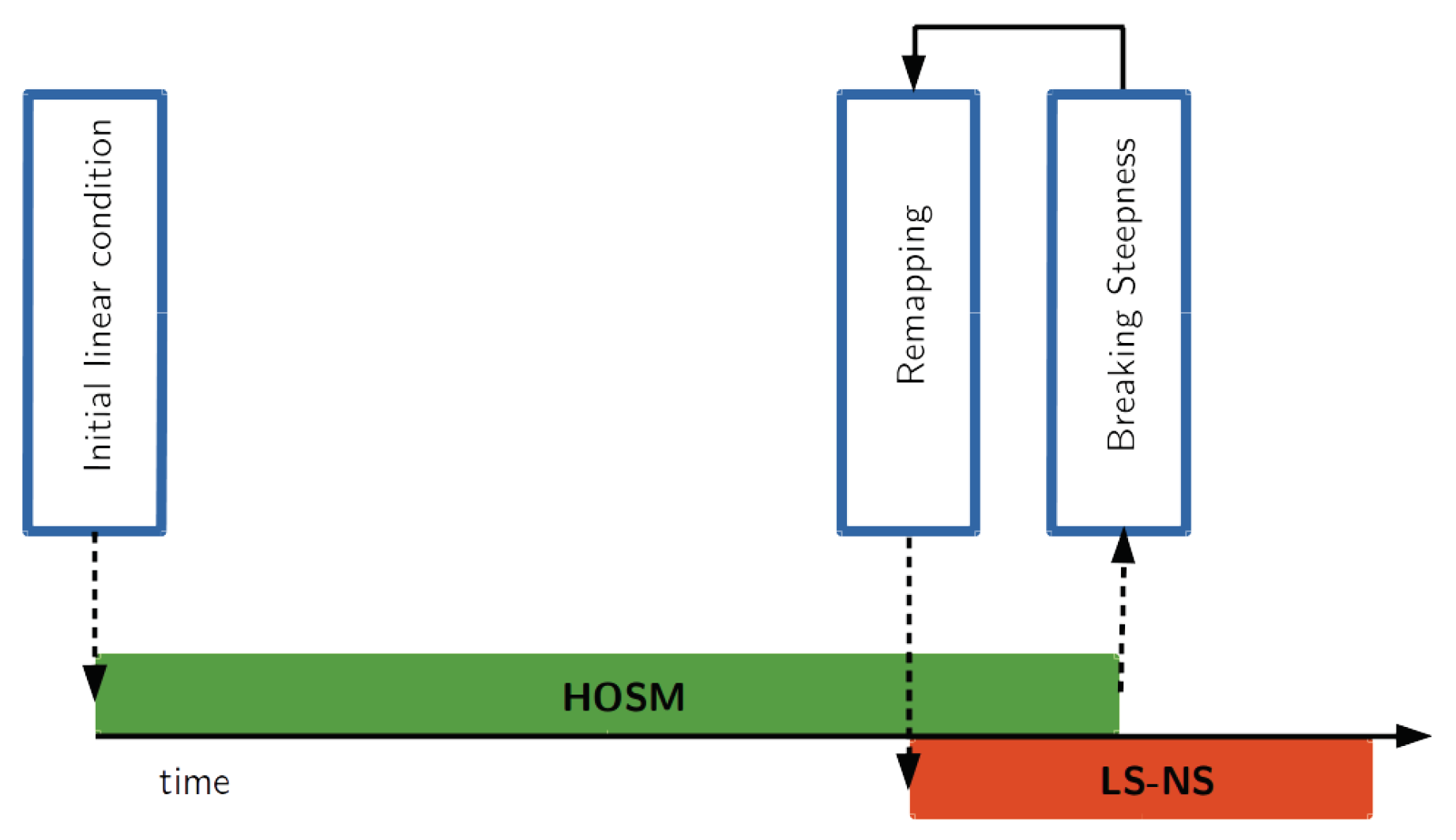
2.1.3. Coupling the HOSM and the LS-NS

Starting from an initial condition the wave evolution is simulated with the HOSM up to one period prior the breaking onset (identified as $ka=0.35$, [42,51]). We note that only the breaking onset injects vorticity in the flow field [35] and potential flow approximation accurately predicts the surface elevation even in presence of strong vorticity prior the breaking onset [52]. Surface elevation and velocity potential obtained from the HOSM at this instant are used to initialise the LS-NS that only simulates the final stages of the breaking (see Figure 1). The coupling allows to significantly reduce the computational time associated with LS-NS simulations [21]. The HOSM fully simulates the nonlinear evolution occurring over tens of wave periods in less than a 1 s CPU time. On the other hand, the LS-NS runs at 1 period of wave simulation for 1 day CPU time on the same machine, i.e., ${10}^5$ times slower than the HOSM.

The procedure is summarised here [36]:

• The HOSM surface elevation and potential at the final instant ($\eta \left(x\right)$ and $\psi \left(x\right)$) are interpolated over a grid compatible with the resolution needed by the LS-NS simulation. This is about 400 elements per wavelength ($L_0$) [50]. A cubic spline with periodic conditions is used to resample the surface elevation and its potential.
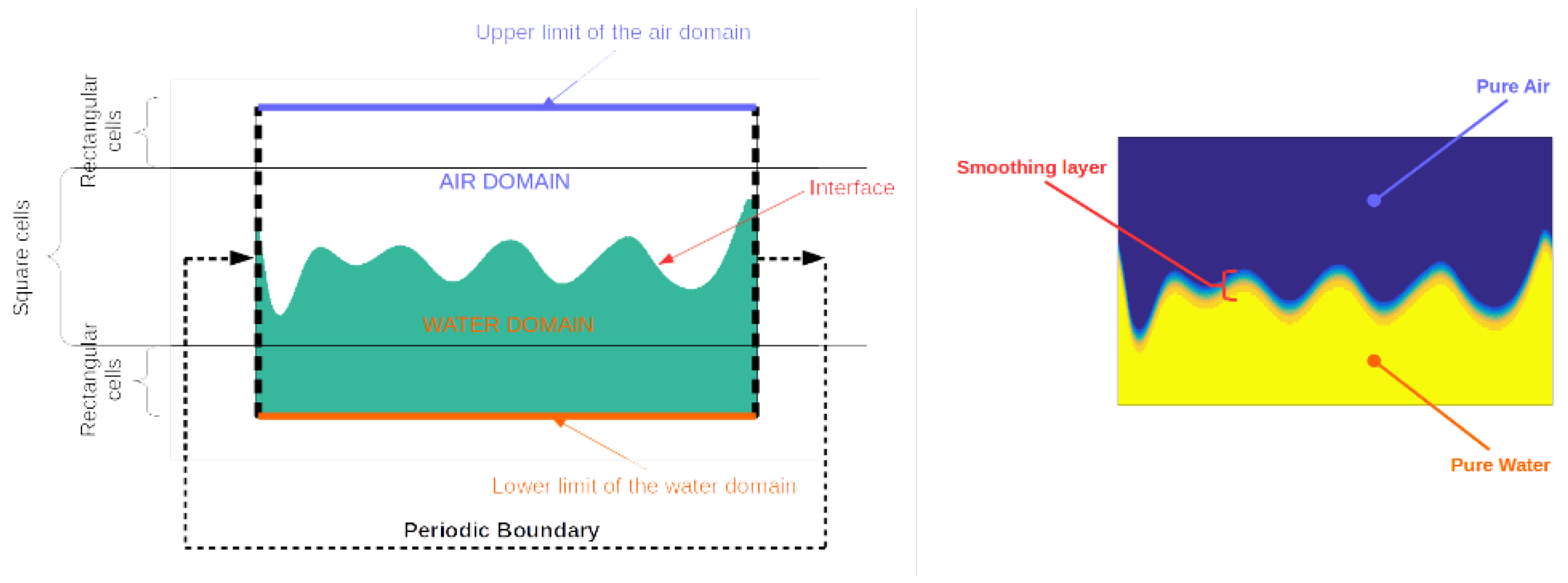
• Surface elevation and velocity potential are only defined at the surface. From the boundary value problem, defined on the contour, the potential at any point in the water domain is reconstructed by using boundary integral representation. The reconstruction is done numerically. The computational domain is discretised with square cells, i.e., dimension in the vertical axis is equal to the horizontal dimension, for $-0.3<z/L_0<0.3$. Out of this layer the vertical dimension is stretched logarithmically, i.e., rectangular cells (see Figure 2). A no slip boundary condition is used to limit the computational domain in $-1<z/L_0<1$.
• To obtain the velocity components in the water domain the spatial derivatives of the potential are computed using a second order finite difference scheme. The value at the centre of the cell, ${\mathbf{x}}_C$, is computed using the four points at ${\mathbf{x}}_D={\mathbf{x}}_C\pm \mathbf{\Delta }/5$. $\mathbf{\Delta }$ denotes the dimension of the cell.
• The boundary value problem is formulated also for the air domain. The boundary of the air domain are the air-water interface (at the bottom), and the arbitrarily chosen limit of the computational domain at the top (indicated in blue in Figure 2). At the free surface the continuity on the normal velocity is enforced providing the necessary Neumann condition for the solution of the boundary value problem. The velocity field in the air is then computed adopting the same methodology used for the water side (point 2. and 3.).
• The signed distance function d is initialised. This is needed for the initialisation of the density distribution in the Level-Set technique. The distance is measured from each grid node to the closest segment defined by two successive points on the resampled free surface. The distance is positive if the grid node is in water, negative in the air side. The Point in Polygon algorithm is used to identify if a grid node belongs to the air or the water side of the domain.
• At the interface between the two fluids (air and water), the velocity component tangential to the free surface has a jump. The discontinuity is consistent with the potential flow theory (no stress condition at the interface) but it does not apply to the two fluid approach. The jump is smoothed by gradually varying the fluid properties (density and viscosity) across the interface. Spurious component that are generated in this layer (∼5 cells, see Figure 2) because of the baroclinic variation of the velocity and of the spreading of the surface tension forces are not propagated in the rest of the domain because the density is reinitialised at each step.

3. Results

3.1. Numerical Simulations

3.1.1. Set-Up and Initial Conditions

In the ocean, modulational instability is the main nonlinear mechanism leading to wave growth and, eventually, breaking [21,51]. This mechanism can be exemplified by the interaction between a monochromatic wave (called carrier) and infinitesimal sidebands perturbations [53]. Energy is nonlinearly exchanged between the carrier and the sidebands resulting in the growth of the perturbations [54,55]. In the physical domain, the energy exchange leads to the formation of a rogue wave from an initially monochromatic wave train [53]. The time and space needed for the instability to develop can be controlled by tuning the frequency and amplitude of the sideband perturbations [56].

In particular, the nonlinear energy exchange is triggered if the Benjamin Feir Instability Index (BFI), an index of nonlinearity, is sufficiently high, i.e., $BFI>1$ [35,53,56]. Under the hypothesis of deep water conditions, the index is computed as [57,58]:

$$BFI=2\sqrt{2}\frac{k_0{A}_0}{\Delta k/k_0}=\sqrt{2}\frac{k_0{A}_0}{\Delta \omega /{\omega }_0}.$$

(6)

Here $k_0$ is the wavenumber of the carrier wave, ${\omega }_0$ the corresponding radial frequency, $\Delta k$ the wavenumber difference between carrier and sideband, $\Delta \omega$ the radial frequency difference between carrier and sideband and $A_0$ the amplitude sum of carrier (a) and sidebands ($b_{\pm }$), i.e., $A_0=a+b_{+}+b_{-}$.

The breaking rogue wave generated via modulational instability is studied numerically. In the simulation, the bandwidth is set to $\Delta k/k_0=1/5$ (equivalent to $\Delta \omega /{\omega }_0=1/10$). The wave group is periodic over 5 waves in the spatial domain and 10 periods in the time domain. The wave period of the carrier is set to $T_0=0.8$ s (${\omega }_0=2\pi /T_0$), the wave steepness $k_0{A}_0=0.1474$ and the perturbation to carrier amplitude ratio $b_{\pm }/a=0.01$. The resulting BFI is 2.08.

The initial surface elevation and the corresponding velocity potential at the surface given to the HOSM are defined respectively as:

$$\eta (x,t=0)=a·cos\left[k_{0}x\right]+b_{\pm }·cos[(k_0\pm \Delta k)x+\pi /4],$$

(7)

$$\begin{array}{c}\psi (x,t=0)=a\sqrt{g/k_0}exp\left(k_0\eta \right)·sin\left[k_{0}x\right]\hfill \\ +b_{\pm }\sqrt{g/(k_0\pm \Delta k)}exp\left((k_0\pm \Delta k)\eta \right)·sin[(k_0\pm \Delta k)x+\pi /4].\hfill \end{array}$$

(8)

For the LS-NS density of the air and water are respectively ${\rho }_a$ = 1.25 kg/m${}^3$ and ${\rho }_w$ = 1000 kg/m${}^3$. Surface tension for pure water is $\sigma$ = 0.0073 N/m and the dynamical viscosity for air and water are ${\mu }_a=1.8\times {10}^{-5}$ Pa·s and ${\mu }_w=1.0\times {10}^{-3}$ Pa·s. We recall that the spatial resolution is over 400 grid points per wavelength (2048 grid points per 5 wavelengths), denser than comparable NS simulations of breaking waves used for engineering purposes [35,36,37,38].

We note that both the HOSM and the LS-NS used here adopt periodic boundary conditions (see Figure 2). This is made possible by the periodicity of the wave group itself. The equivalence between evolution in space and time has been commonly adopted (and proved) in the past [59]. We note that formally the periodic solution does not correspond to the wave evolution in a physical wave flume and, despite being a limitation of the present study, allows to make NS simulations considerably faster.

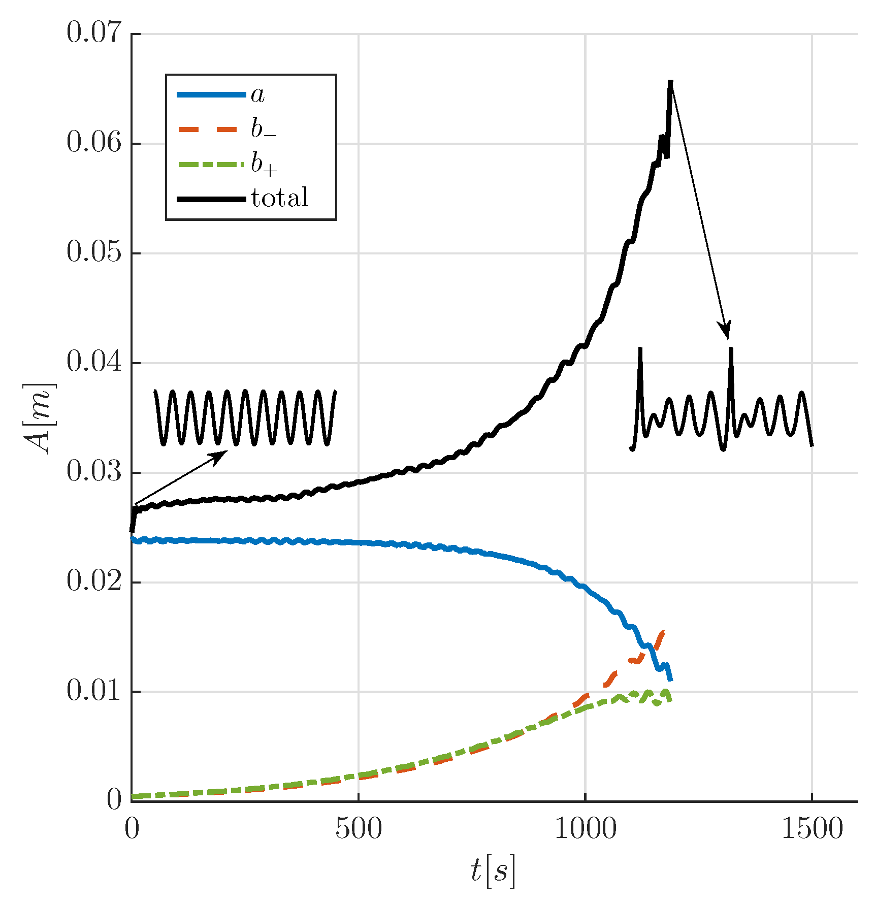
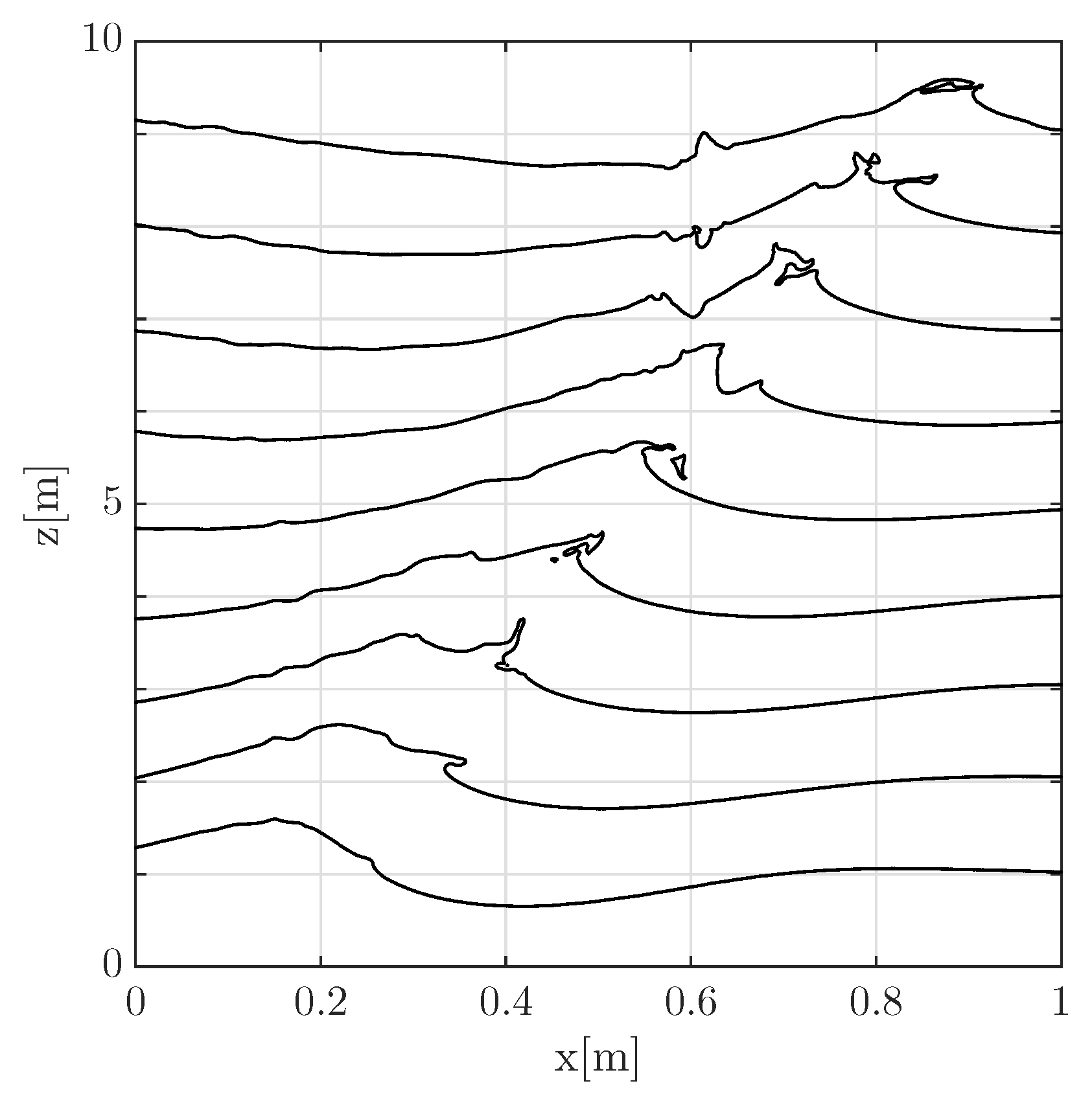
3.1.2. Wave Evolution

The evolution of the maximum amplitude in the wave group (A) as obtained from the HOSM is shown in Figure 3. At breaking, which occurs at about 1200 s from the HOSM initialisation and local wave steepness of 0.35, the envelope has grown by about two times compared to the initial monochromatic wave. The left sideband ($b_{-}$) has outgrown the carrier wave (a), see Figure 3.

After the switch from the HOSM to the NS, the evolution of the breaking wave is shown in Figure 4. At the breaking, a jet develops at the front of the largest wave in the group (the one shown in the plot).

As expected, the largest horizontal velocities are concentrated at the top of the crest where the overturning movement is taking place (see Figure 5). The figure also highlights asymmetries in the wave shape and the associated velocity field. It is worth noticing that the velocity in air is not shown for the sake of clarity.

In previous laboratory experiments, the shape of the breaking wave has been found to be affected by the presence of surfactant that might modify the surface tensions [60]. For this reason a sensitivity analysis in respect of viscosity and surface tension is performed. To exaggerate the effect variation of this parameters have on the solution, viscosity and surface tension are varied singularly by ±30%. Results are summarised in Figure 6.

Viscosity and surface tension can affect velocities up to $\pm 0.1$ m/s (about 10% of the maximum crest velocity). Viscosity has a much stronger effect on both the jet shape and the flow field. Note, however, that in all the cases the wave profile, with the exception of the jet, remains unaffected by variation of the physical parameters.

3.2. Laboratory Experiment

3.2.1. Set-Up and Initial Conditions

A physical experiment is conducted in the Extreme Air Sea Interaction facility (EASI) using the same set-up described in [11,12,22]. The flume is 60 m long, 2 m wide and filled up to a depth of 0.9 m. At one end waves are generated by a cylindrical wave maker and the opposite end a linear beach absorbs the incoming wave energy. The surface elevation is monitored with a number of wave probes deployed along the tank. The Particle Image Velocimetry (PIV) setup for the fluid velocity measurements is located 34 m from the wave maker in correspondence of a glass window that guarantees optical access. The field of view is approximately 170 mm × 200 mm with a resolution of ≈ 0.1 mm/px [11,12]. The experiment is performed to replicate the breaking event generated numerically. However, the notable difference is that the numerical simulation is performed with periodic boundary conditions, on the other hand experiments are conducted in a wave flume. The imposed surface at the wave-maker is:

$$\eta (x=0,t)=a·sin\left[{\omega }_{0}t\right]+b_{\pm }·sin[({\omega }_0\pm \Delta \omega )t-\pi /4].$$

(9)

To reproduce the numerical simulation the same dominant wave period is used ($T_0=0.8$ s). Due to the limited length of the wave flume, the initial condition in the flume starts from a more advanced stage of evolution compared to the one used during the numerical simulation. In particular, amplitudes of the sidebands and initial steepness need to be tuned to obtain the wave breaking in the PIV field of view [11,12,22]. The initial sideband to carrier amplitude ratio is set $b_{\pm }/a=0.10$ (cf. 0.01 in the numerical simulation) and the corresponding initial steepness is $k_{0}A=0.1734$.

PIV processing is performed using the software PIVLAb [61]. Images pairs are sampled every $\Delta t=2.5$ ms. To obtain robust statistical results the test is repeated 20 times.

3.2.2. Wave Evolution

The evolution of the maximum amplitude at different distances from the wave maker is shown in Figure 7. The partitioning of the energy between carrier and sidebands is also shown. Starting from a carrier (a) more energetic than the sidebands close to the wave maker, modulational instability leads to the growth of the left side-band ($b_{-}$) that eventually outgrows the carrier consistently with the HOSM simulation. The shape of the wave train is shown in the insets, an extreme wave forms from an initially slightly modulated wave train. At the breaking (recorded at the fifth probe) a sudden drop of energy occurs. Note that energy exchanges between wave components continue after the breaking.

4. Discussion

The comparison between the simulations and the experiments focusses on the horizontal velocity field under the breaking event. The major difference between physical experiments and the numerical simulations is the shape of the breaking wave, see Figure 8. In the numerical simulation (red line in Figure 8) a jet departs from the tip of the crest. In the experiment (black particles in Figure 8) the jet is far less pronounced. The surface elevation of the wave front is reproduced correctly by the simulations.

It is important to note that the interface in the Level-Set method is identified by $\rho =500$ kg/m${}^3$ (this value is the average between the density of pure air and pure water). For this reason the jet identified numerically is a mixture of air and water, i.e., density in the jet are below the density of pure water. To better resolve the foamy jet a much smaller grid size would be required making the simulations unfeasible for practical engineering purposes. However, a finer grid is prone to numerical artefacts and would increase the computational time. To account for the variable density across the interface, velocities are corrected multiplying by the density ratio $\rho /{\rho }_W$. Only data points where the density ratio is higher than 0.5 are considered as belonging to the water side.

Velocities in the water have similar topology in experiments and simulations, i.e., higher velocity are recorded closer to the top of the wave crest. In the experiments the highest horizontal velocities are concentrated towards the front of the breaking wave (see left panel in Figure 8 noting that the velocity in the crest region is highly variable [21] and PIV uncertainty up to 33% [11,12]), in the simulation velocities at the air-water interface are smaller. It must be recalled that in the LS the fluid properties jump and the surface tension forces are spread across a a finite region about he interface, which affects the accuracy of the velocity in this transition zone.

The velocity obtained numerically and experimentally under the wave crest are compared in Figure 9. Overall, experiments provide larger velocities than those obtained numerically. The difference is about 10% (dashed line in Figure 9) in the wave body where both simulations and measurements are available which is not statistically significant due to measurement uncertainties [11,12]. The inset in Figure 9 highlights how the largest velocity differences are localised in the top of the crest and the front face of the wave. Close to the interface the numerical simulation fails to accurately reproduce the velocity field due to the interface treatment but also PIV measurements become challenging [11,12].

The velocity profile beneath the wave crest is extracted from simulations and experiments. As a reference, in Figure 10, the velocity profile is plotted against engineering methods developed to obtain the velocity only from the surface elevation time history. The Grue method, for which the velocity profile can be approximated by a third order monochromatic Stokes wave with the same amplitude and period [19], and Donelan method, in which the contribution of each spectral component is iteratively added to the perturbed solution [23], are compared. These two methods have been shown to provide good agreement with experimental results [12].

The velocity profiles highlight that experiments provide larger values compared to the simulations, the difference is less than 0.1 m/s. PIV reconstructs the velocity profile up to elevations very close to the top of the wave, however reflections at the interface make the image processing challenging [11,12]. On the other hand, the LS-NS accurately identifies the surface but the velocity and density close to the interface are uncertain due to the smoothing of properties across the interface itself. For this reasons the velocity is only reported up to about 5 cm (the maximum wave elevation is 6 cm). The Grue and Donelan method used to estimate the velocity profile from the measurements in this case provide an upper and lower limit for the numerical and experimental measurements. At the tip of the crest the Grue and Donelan methods predict the same maximum velocity. In this case, the Grue method accurately predicts the experimental data (cf. [12,21] in which the agreement is far from optimal).

5. Conclusions

A breaking wave induced by modulational instability has been generated both numerically and experimentally to evaluate the numerical solver results in regard of the induced fluid motion. To speed-up the simulations, Navier–Stokes (NS) are initialised from a pre-breaking solution obtained using the Higher Order Spectral Method (HOSM). The coupling of a “fast” method (HOSM) with a “slow” method (NS) allows one to reduce the computational time and, at the same time, accurately reproduce the breaking stage starting from a fully nonlinear wave condition that better reproduces ocean conditions. Whereas the HOSM only takes few seconds to simulate the entire evolution, the present NS solver is not particularly efficient and takes about a week of single processor CPU time to simulate one wave period. The general methodology presented in the manuscript can be used when the NS are coupled with the impact on a structure or a range of engineering problems that require the post-breaking dynamics (which we plan to study in future).

Comparison of the numerical simulation with the physical experiments highlights that the wave evolution is comparable and the shape of the breaking wave is accurately reproduced, despite having used a periodic support for the numerical simulations (to reduce the domain size and speed up the numerical simulation). A notable exception is the jet, that is absent in physical experiments. It is worth noting that the shape of the jet itself has been found to highly depend on the choice of the physical parameters, i.e., surface tension and viscosity.

Overall, the topology of the flow field recorded in the experiments is in reasonable agreement with the one obtained from numerical simulations. However, significant differences are observed in the velocity close to the crest (about 10%). Despite having ensured the equivalence between spatial and time evolution (in the wave tank and in the numerical simulation respectively), it cannot be ruled out that the periodic boundary condition might have been responsible for the velocity difference between experiments and simulations together with the relatively low spatial resolution (e.g., De Vita et al. [54] uses 5 times more elements per wavelength) and to the spreading of the fluid properties. In this regard, we note that in the LS the interface is correctly identified even at relatively low resolution, but the velocity at the interface is more sensitive to the grid size. Attempts to overcome limitations highlighted in this work are currently under development. In particular, it is advisable a comparison with simulations based on a numerical wave tank configuration to verify if the periodic support is a viable approximation for engineering purposes.

Application of engineering method to predict the velocity profile beneath the crest shows that, in this case, the Grue method accurately reproduces the velocity profile measured during the laboratory experiments, while the Donelan method accurately reproduces the LS velocity profile up to the mean water level.

References

1. Bitner-Gregersen, E.; Toffoli, A. Occurrence of rogue sea states and consequences for marine structures. Ocean Dyn. 2014, 64, 1457–1468. [Google Scholar] [CrossRef]
2. Liu, P. A chronology of freauqe wave encounters. Geofizika 2007, 24, 57–70. [Google Scholar]
3. Nikolkina, I.; Didenkulova, I. Rogue waves in 2006–2010. Nat. Hazards Earth Syst. Sci. 2011, 11, 2913–2924. [Google Scholar] [CrossRef] [Green Version]
4. Cavaleri, L.; Bertotti, L.; Torrisi, L.; Bitner-Gregersen, E.; Serio, M.; Onorato, M. Rogue waves in crossing seas: The Louis Majesty accident. J. Geophys. Res. Ocean. 2012, 117. [Google Scholar] [CrossRef] [Green Version]
5. Longuet-Higgins, M. Breaking waves in deep or shallow water. In Proceedings of the 10th Conference on Naval Hydrodynamics, Cambridge, MA, USA, 24–28 June 1974; Volume 597. [Google Scholar]
6. Tromans, P.; Anaturk, A.; Hagemeijer, P. A new model for the kinematics of large ocean waves-application as a design wave. In Proceedings of the First International Offshore and Polar Engineering Conference, Edinburgh, UK, 11–16 August 1991. [Google Scholar]
7. Faltinsen, O. Sea Loads on Ships and Offshore Structures; Cambridge University Press: Cambridge, UK, 1993; Volume 1. [Google Scholar]
8. Clauss, G.; Klein, M. The New Year Wave in a seakeeping basin: Generation, propagation, kinematics and dynamics. Ocean Eng. 2011, 38, 1624–1639. [Google Scholar] [CrossRef]
9. Onorato, M.; Proment, D.; Clauss, G.; Klein, M. Rogue waves: From nonlinear Schrödinger breather solutions to sea-keeping test. PLoS ONE 2013, 8, e54629. [Google Scholar] [CrossRef]
10. Zhang, H.; Guedes Soares, C. Ship responses to abnormal waves simulated by the Nonlinear Schrödinger Equation. Ocean Eng. 2016. [Google Scholar] [CrossRef]
11. Alberello, A.; Chabchoub, A.; Babanin, A.; Monty, J.; Lee, J.; Elsnab, J.; Bitner-Gregersen, E.; Toffoli, A. The Velocity Field Underneath Linear and Nonlinear Breaking Rogue Waves. In Proceedings of the ASME 2016 35th International Conference on Offshore Mechanics and Arctic Engineering, Busan, Korea, 19–24 June 2016. [Google Scholar]
12. Alberello, A.; Chabchoub, A.; Monty, J.P.; Nelli, F.; Lee, J.H.; Elsnab, J.; Toffoli, A. An experimental comparison of velocities underneath focussed breaking waves. Ocean Eng. 2018, 155, 201–210. [Google Scholar] [CrossRef] [Green Version]
13. Chaplin, J.; Rainey, R.; Yemm, R. Ringing of a vertical cylinder in waves. J. Fluid Mech. 1997, 350, 119–147. [Google Scholar] [CrossRef]
14. Grue, J. On four highly nonlinear phenomena in wave theory and marine hydrodynamics. Appl. Ocean Res. 2002, 24, 261–274. [Google Scholar] [CrossRef]
15. Wienke, J.; Oumeraci, H. Breaking wave impact force on a vertical and inclined slender pile—Theoretical and large-scale model investigations. Coast. Eng. 2005, 52, 435–462. [Google Scholar] [CrossRef]
16. Morison, J.; Johnson, J.; Schaaf, S. The force exerted by surface waves on piles. J. Pet. Technol. 1950, 2, 149–154. [Google Scholar] [CrossRef]
17. Goda, Y. Random Seas and Design of Maritime Structures; World Scientific: London, UK, 2010. [Google Scholar]
18. Alberello, A.; Chabchoub, A.; Gramstad, O.; Babanin, A.V.; Toffoli, A. Non-Gaussian properties of second-order wave orbital velocity. Coast. Eng. 2016, 110, 42–49. [Google Scholar] [CrossRef] [Green Version]
19. Grue, J.; Clamond, D.; Huseby, M.; Jensen, A. Kinematics of extreme waves in deep water. Appl. Ocean Res. 2003, 25, 355–366. [Google Scholar] [CrossRef] [Green Version]
20. Grue, J.; Jensen, A. Experimental velocities and accelerations in very steep wave events in deep water. Eur. J. Mech. B Fluids 2006, 25, 554–564. [Google Scholar] [CrossRef]
21. Alberello, A.; Pakodzi, C.; Nelli, F.; Bitner-Gregersen, E.M.; Toffoli, A. Three dimensional velocity field underneath a breaking rogue wave. In Proceedings of the ASME 2017 36th International Conference on Ocean, Offshore and Arctic Engineering, Trondheim, Norway, 25–30 June 2017. [Google Scholar]
22. Lee, J.H.; Monty, J.P.; Elsnab, J.; Toffoli, A.; Babanin, A.V.; Alberello, A. Estimation of Kinetic Energy Dissipation from Breaking Waves in the Wave Crest Region. J. Phys. Oceanogr. 2017, 47, 1145–1150. [Google Scholar] [CrossRef]
23. Donelan, M.; Anctil, F.; Doering, J. A simple method for calculating the velocity field beneath irregular waves. Coast. Eng. 1992, 16, 399–424. [Google Scholar] [CrossRef]
24. Stansberg, C.; Gudmestad, O.; Haver, S. Kinematics under extreme waves. J. Offshore Mech. Arct. Eng. 2006, 130, 021010. [Google Scholar] [CrossRef]
25. Iafrati, A. Numerical study of the effects of the breaking intensity on wave breaking flows. J. Fluid Mech. 2009, 622, 371–411. [Google Scholar] [CrossRef]
26. Jacobsen, N.; Fuhrman, D.; Fredsøe, J. A Wave Generation Toolbox for the Open-Source CFD Library: OpenFOAM®. Int. J. Numerl. Meth. Fluids 2012, 70, 1073–1088. [Google Scholar] [CrossRef]
27. Higuera, P.; Lara, J.; Losada, I. Simulating coastal engineering processes with OpenFOAM. Coast. Eng. 2013, 71, 119–134. [Google Scholar] [CrossRef]
28. Alagan Chella, M.; Bihs, H.; Myrhaug, D.; Muskulus, M. Hydrodynamic characteristics and geometric properties of plunging and spilling breakers over impermeable slopes. Ocean Model. 2016, 103, 53–72. [Google Scholar] [CrossRef]
29. Popinet, S. Gerris: A tree-based adaptive solver for the incompressible Euler equations in complex geometries. J. Comput. Phys. 2003, 190, 572–600. [Google Scholar] [CrossRef]
30. Hirt, C.; Nichols, B. Volume of Fluid (VOF) method for the dynamics of free boundaries. J. Comput. Phys. 1981, 39, 201–225. [Google Scholar] [CrossRef]
31. Osher, S.; Sethian, J. Fronts propagating with curvature-dependent speed: Algorithms based on Hamilton-Jacobi formulations. J. Comput. Phys. 1988, 79, 12–49. [Google Scholar] [CrossRef] [Green Version]
32. Sussman, M.; Smereka, P.; Osher, S. A level set approach for computing solutions to incompressible two-phase flow. J. Comput. Phys. 1994, 114, 146–159. [Google Scholar] [CrossRef]
33. Vogt, M.; Larsson, L. Level set methods for predicting viscous free surface flows. In Proceedings of the 7th International Conference on Numerical Ship Hydrodynamics, Nantes, France, 19–22 July 1999. [Google Scholar]
34. Banner, M.; Peirson, W. Wave breaking onset and strength for two-dimensional deep-water wave groups. J. Fluid Mech. 2007, 585, 93–115. [Google Scholar] [CrossRef]
35. Iafrati, A.; Babanin, A.; Onorato, M. Modulational instability, wave breaking, and formation of large-scale dipoles in the atmosphere. Phys. Rev. Lett. 2013, 110, 184504. [Google Scholar] [CrossRef]
36. Iafrati, A.; Babanin, A.; Onorato, M. Modeling of ocean–atmosphere interaction phenomena during the breaking of modulated wave trains. J. Comput. Phys. 2014, 271, 151–171. [Google Scholar] [CrossRef]
37. Perić, R.; Hoffmann, N.; Chabchoub, A. Initial wave breaking dynamics of Peregrine-type rogue waves: A numerical and experimental study. Eur. J. Mech. B Fluids 2015, 49, 71–76. [Google Scholar] [CrossRef] [Green Version]
38. Vyzikas, T.; Deshoulières, S.; Giroux, O.; Barton, M.; Greaves, D. Numerical study of fixed Oscillating Water Column with RANS-type two-phase CFD model. Renew. Energy 2016. [Google Scholar] [CrossRef]
39. Dommermuth, D.G.; Yue, D.K.P.; Lin, W.M.; Rapp, R.J.; Chan, E.S.; Melville, W.K. Deep-water plunging breakers: A comparison between potential theory and experiments. J. Fluid Mech. 1988, 189, 423–442. [Google Scholar] [CrossRef]
40. Skyner, D. A comparison of numerical predictions and experimental measurements of the internal kinematics of a deep-water plunging wave. J. Fluid Mech. 1996, 315, 51–64. [Google Scholar] [CrossRef]
41. Emarat, N.; Forehand, D.I.; Christensen, E.D.; Greated, C.A. Experimental and numerical investigation of the internal kinematics of a surf-zone plunging breaker. Eur. J. Mech. B Fluids 2012, 32, 1–16. [Google Scholar] [CrossRef]
42. Iafrati, A.; De Vita, F.; Toffoli, A.; Alberello, A. Strongly nonlinear phenomena in water waves. Trans. SNAME 2015, 123, 17–38. [Google Scholar]
43. Iafrati, A. Energy dissipation mechanisms in wave breaking processes: Spilling and highly aerated plunging breaking events. J. Geophys. Res. Ocean. 2011, 116. [Google Scholar] [CrossRef]
44. West, B.; Brueckner, K.; Janda, R.; Milder, D.; Milton, R. A new numerical method for surface hydrodynamics. J. Geophys. Res. Ocean. 1987, 92, 11803–11824. [Google Scholar] [CrossRef]
45. Dommermuth, D.; Yue, D. A high-order spectral method for the study of nonlinear gravity waves. J. Fluid Mech. 1987, 184, 267–288. [Google Scholar] [CrossRef]
46. Toffoli, A.; Bitner-Gregersen, E.; Onorato, M.; Babanin, A. Wave crest and trough distributions in a broad-banded directional wave field. Ocean Eng. 2008, 35, 1784–1792. [Google Scholar] [CrossRef]
47. Toffoli, A.; Benoit, M.; Onorato, M.; Bitner-Gregersen, E. The effect of third-order nonlinearity on statistical properties of random directional waves in finite depth. Nonlinear Process. Geophys. 2009, 16, 131–139. [Google Scholar] [CrossRef] [Green Version]
48. Courant, R.; Friedrichs, K.; Lewy, H. On the partial difference equations of mathematical physics. IBM J. Res. Dev. 1967, 11, 215–234. [Google Scholar] [CrossRef]
49. Iafrati, A.; Di Mascio, A.; Campana, E. A level set technique applied to unsteady free surface flows. Int. J. Numer. Methods Fluids 2001, 35, 281–297. [Google Scholar] [CrossRef]
50. Iafrati, A.; Campana, E. Free-surface fluctuations behind microbreakers: Space–time behaviour and subsurface flow field. J. Fluid Mech. 2005, 529, 311–347. [Google Scholar] [CrossRef]
51. Babanin, A. Breaking and Dissipation of Ocean Surface Waves; Cambridge University Press: Cambridge, UK, 2011. [Google Scholar]
52. Alberello, A.; Onorato, M.; Frascoli, F.; Toffoli, A. Observation of turbulence and intermittency in wave-induced oscillatory flows. Wave Motion 2019, 84, 81–89. [Google Scholar] [CrossRef]
53. Benjamin, T.; Feir, J. The disintegration of wave trains on deep water Part 1. Theory. J. Fluid Mech. 1967, 27, 417–430. [Google Scholar] [CrossRef]
54. De Vita, F.; Verzicco, R.; Iafrati, A. Breaking of modulated wave groups: Kinematics and energy dissipation processes. J. Fluid Mech. 2018, 855, 267–298. [Google Scholar] [CrossRef]
55. Iafrati, A.; Vita, F.D.; Verzicco, R. Effects of the wind on the breaking of modulated wave trains. Eur. J. Mech. B Fluids 2019, 73, 6–23. [Google Scholar] [CrossRef]
56. Tulin, M.; Waseda, T. Laboratory observations of wave group evolution, including breaking effects. J. Fluid Mech. 1999, 378, 197–232. [Google Scholar] [CrossRef]
57. Janssen, P. Nonlinear four-wave interactions and freak waves. J. Phys. Oceanogr. 2003, 33, 863–884. [Google Scholar] [CrossRef]
58. Onorato, M.; Osborne, A.; Serio, M.; Cavaleri, L.; Brandini, C.; Stansberg, C. Observation of strongly non-Gaussian statistics for random sea surface gravity waves in wave flume experiments. Phys. Rev. E 2004, 70, 067302. [Google Scholar] [CrossRef]
59. Ducrozet, G.; Bonnefoy, F.; Ferrant, P. On the equivalence of unidirectional rogue waves detected in periodic simulations and reproduced in numerical wave tanks. Ocean Eng. 2016, 117, 346–358. [Google Scholar] [CrossRef]
60. Liu, X.; Duncan, J. The effects of surfactants on spilling breaking waves. Nature 2003, 421, 520–523. [Google Scholar] [CrossRef]
61. Thielicke, W.; Stamhuis, E. PIVlab–Towards user-friendly, affordable and accurate digital particle image velocimetry in MATLAB. J. Open Res. Softw. 2014, 2, e30. [Google Scholar] [CrossRef]
Figure 1. Schematic of the coupling between the Higher Order Spectral Method (HOSM) and the Level-Set Navier–Stokes (LS-NS).
Fluids 04 00068 g001
Figure 2. Schematic of the computational domain (on the left) and shematic showing the smoothing layer across the interface (on the right).
Fluids 04 00068 g002
Figure 3. Evolution of the maximum elevation and subdivision into the three initial spectral components (a, b , b + ) extracted from the HOSM simulation. The shape of the surface elevation (in the spatial domain) at the start and at the end of the simulation is also depicted in the insets.
Fluids 04 00068 g003
Figure 4. Surface elevation as obtained from the NS simulations after switching from the HOSM solution. Vertical dimension is amplified by a factor 10 and profiles are shifted vertically by 1 m for readability. The time between the plotted profiles is 0.08 s.
Fluids 04 00068 g004
Figure 5. The velocity field under a breaking wave.
Fluids 04 00068 g005
Figure 6. The effect of viscosity and surface tension on the velocity field under a breaking wave, the difference between horizontal velocity computed with physical parameters and modified parameters is shown. Top left surface tension is decreased by 30% ( s 30 % ), top right surface tension is increased by 30% ( s + 30 % ), bottom left air and water viscosity are decreased by 30% ( v 30 % ), bottom right air and water viscosity are increased by 30% ( v + 30 % ). The red line shows the profile obtained using “physical” parameters.
Fluids 04 00068 g006
Figure 7. Evolution of the maximum elevation and subdivision into the three initial spectral components (a, b , b + ) extracted from the surface elevation recordings. The shape of the surface elevation (in the time domain) at the first probe and at the breaking (vertical dashed line) is also depicted in the insets.
Fluids 04 00068 g007
Figure 8. Horizontal velocity component under breaking wave; Particle Image Velocimetry (PIV) measurements on the left, LS simulations on the right. In black is the profile as detected from the camera images, in red the one obtained by the simulations.
Fluids 04 00068 g008
Figure 9. Scatter plot of the velocity detected from PIV measurements (vertical axis) and Simulations (horizontal axis). The dashed line is the least square linear interpolation, the continuous line is the equivalence line. The inset shows the contour of the velocity difference, i.e., U L S U P I V .
Fluids 04 00068 g009
Figure 10. Velocity profiles extracted from the experiments (circles) and the simulations (dots). Standard engineering predictions extracted from the measured surface time history are also reported for comparison: Grue method (dashed), Donelan method (dash-dotted).
Fluids 04 00068 g010