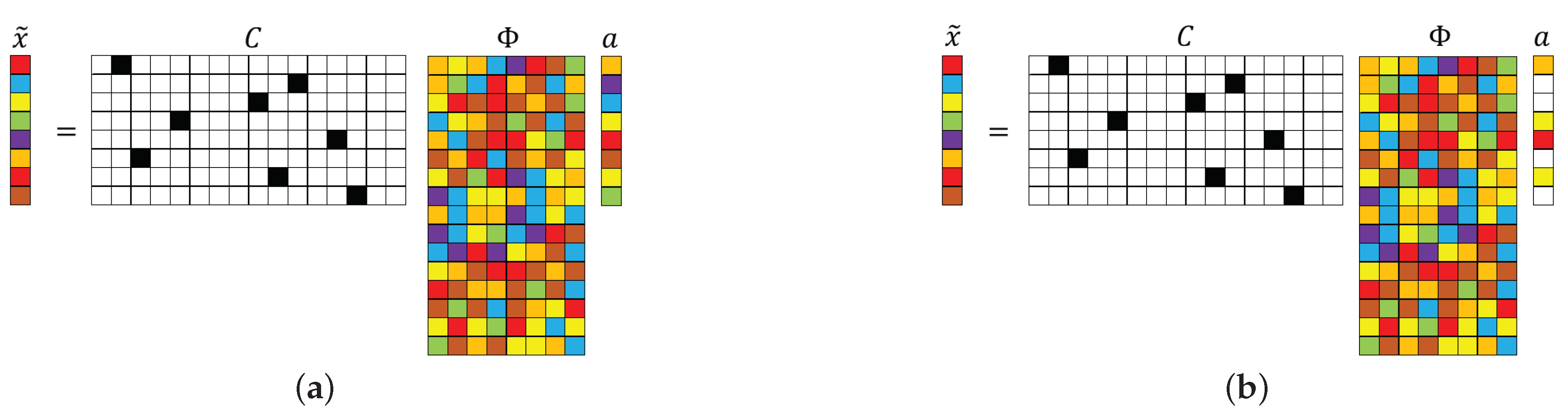
Figure 1.
Schematic illustration of (a) and (b) minimization reconstruction for sparse recovery using a single-pixel measurement matrix. The numerical values in C are represented by colors: black (1) and white (0). The other colors represent numbers that are neither 0 nor 1. In the above schematics, , , and , where . The number of colored cells in a represents the system sparsity K. We note that, for , the method of choice is and, for K smaller than , the method of choice is .
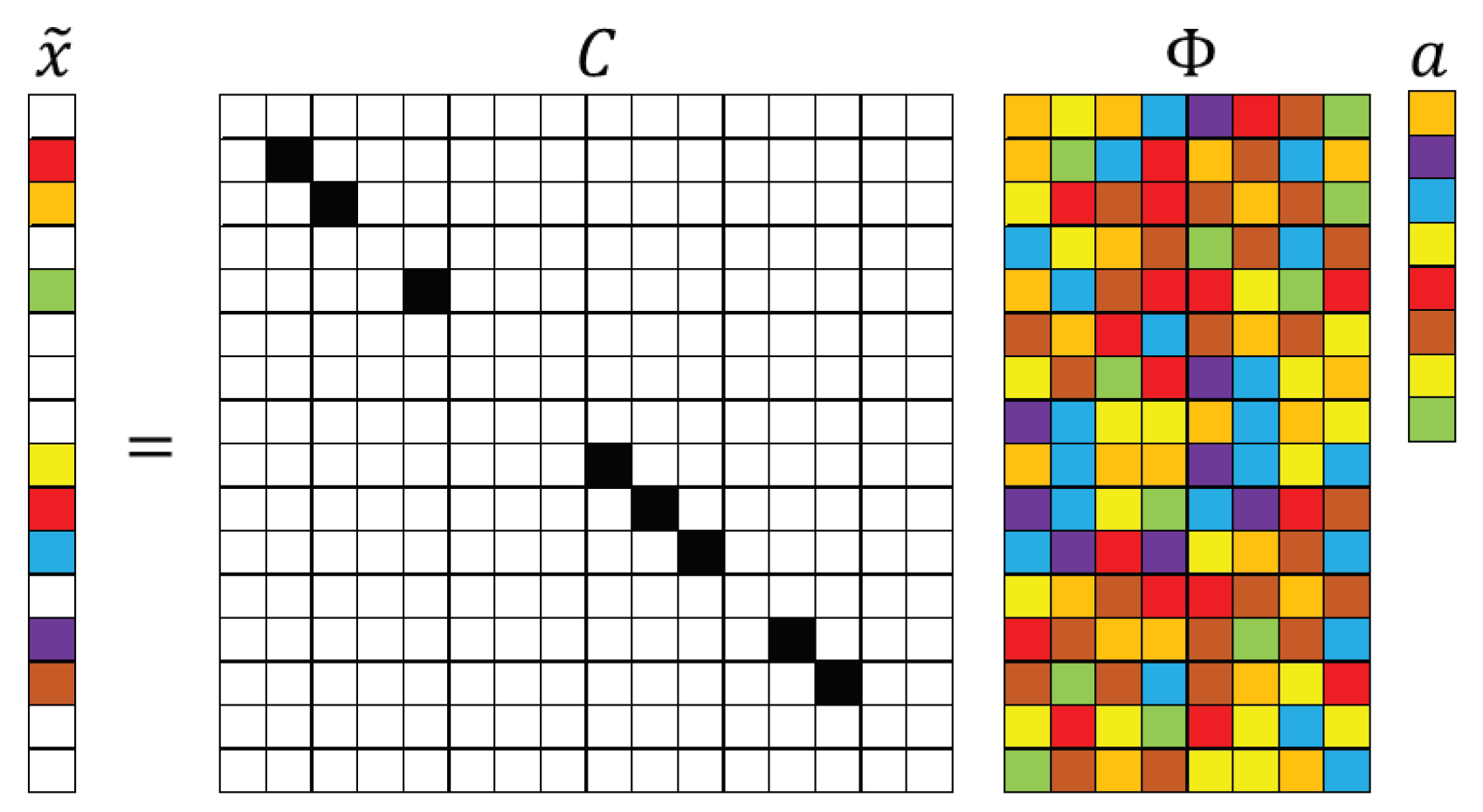
Figure 2.
Schematic illustration of sparse sensor placement. The pastel colored rectangles represent rows activated by the sensors denoted in the measurement matrix through dark squares.
Figure 2.
Schematic illustration of sparse sensor placement. The pastel colored rectangles represent rows activated by the sensors denoted in the measurement matrix through dark squares.
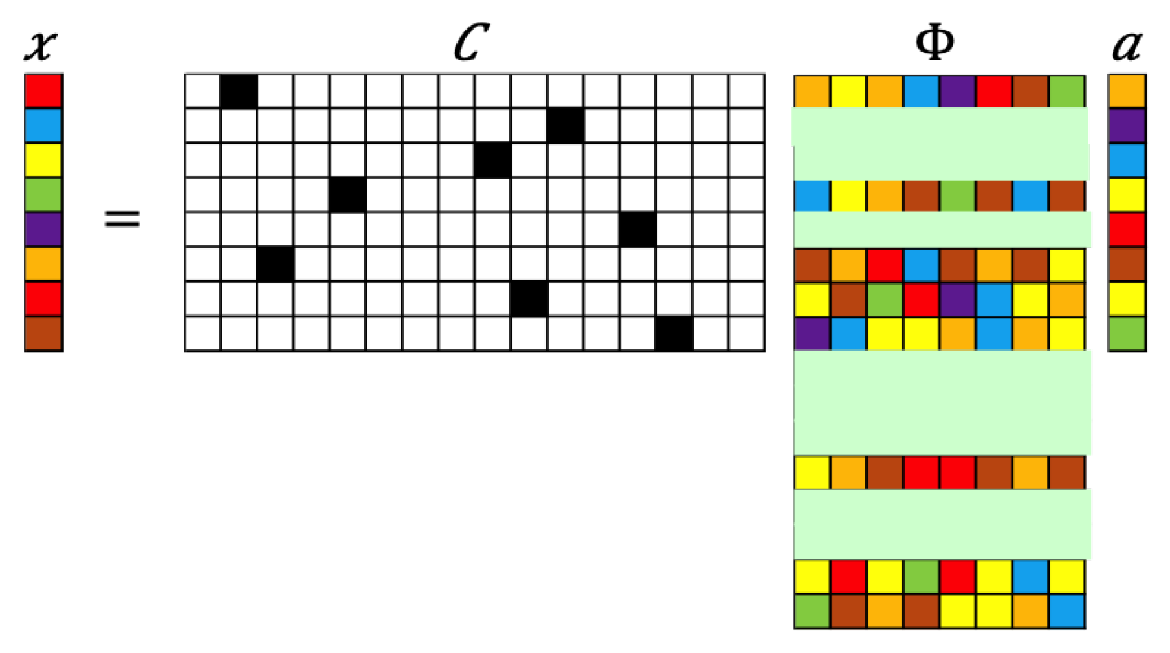
Figure 3.
Schematic of GPOD formulation for sparse recovery. The numerical values represented by the colored blocks: black (1), white (0), and color (other numbers).
Figure 3.
Schematic of GPOD formulation for sparse recovery. The numerical values represented by the colored blocks: black (1), white (0), and color (other numbers).
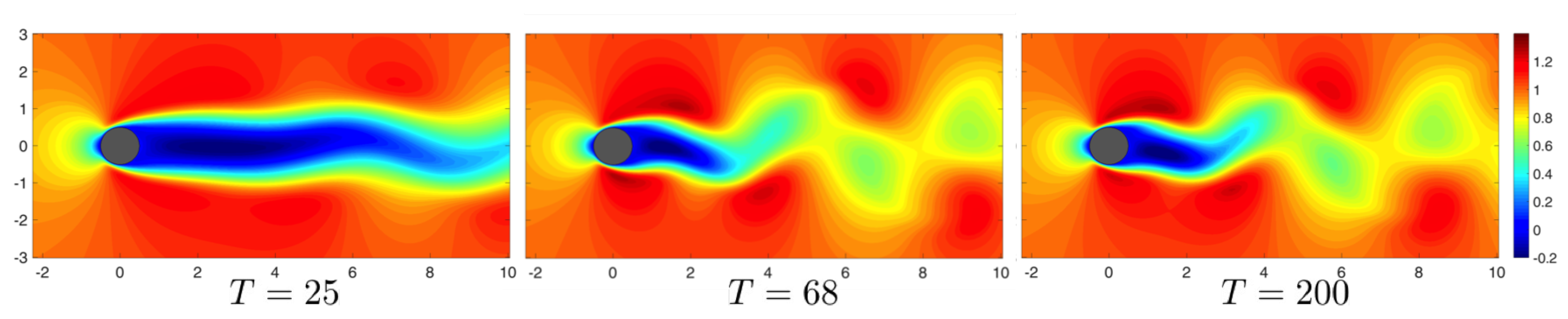
Figure 4.
Isocontour plots of the stream-wise velocity component for the cylinder flow at at show evolution of the flow field. Here, T represents the time non-dimensionalized by the advection time-scale.
Figure 4.
Isocontour plots of the stream-wise velocity component for the cylinder flow at at show evolution of the flow field. Here, T represents the time non-dimensionalized by the advection time-scale.
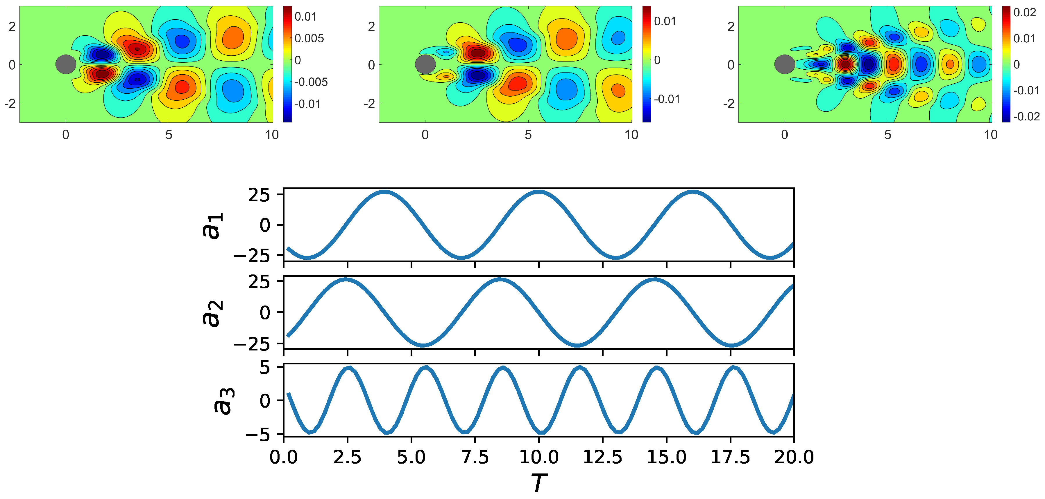
Figure 5.
Isocontours of the three most energetic modes (first row from left to right) and time evolution of the first three POD coefficients (second row) for the cylinder wake flow at .
Figure 5.
Isocontours of the three most energetic modes (first row from left to right) and time evolution of the first three POD coefficients (second row) for the cylinder wake flow at .
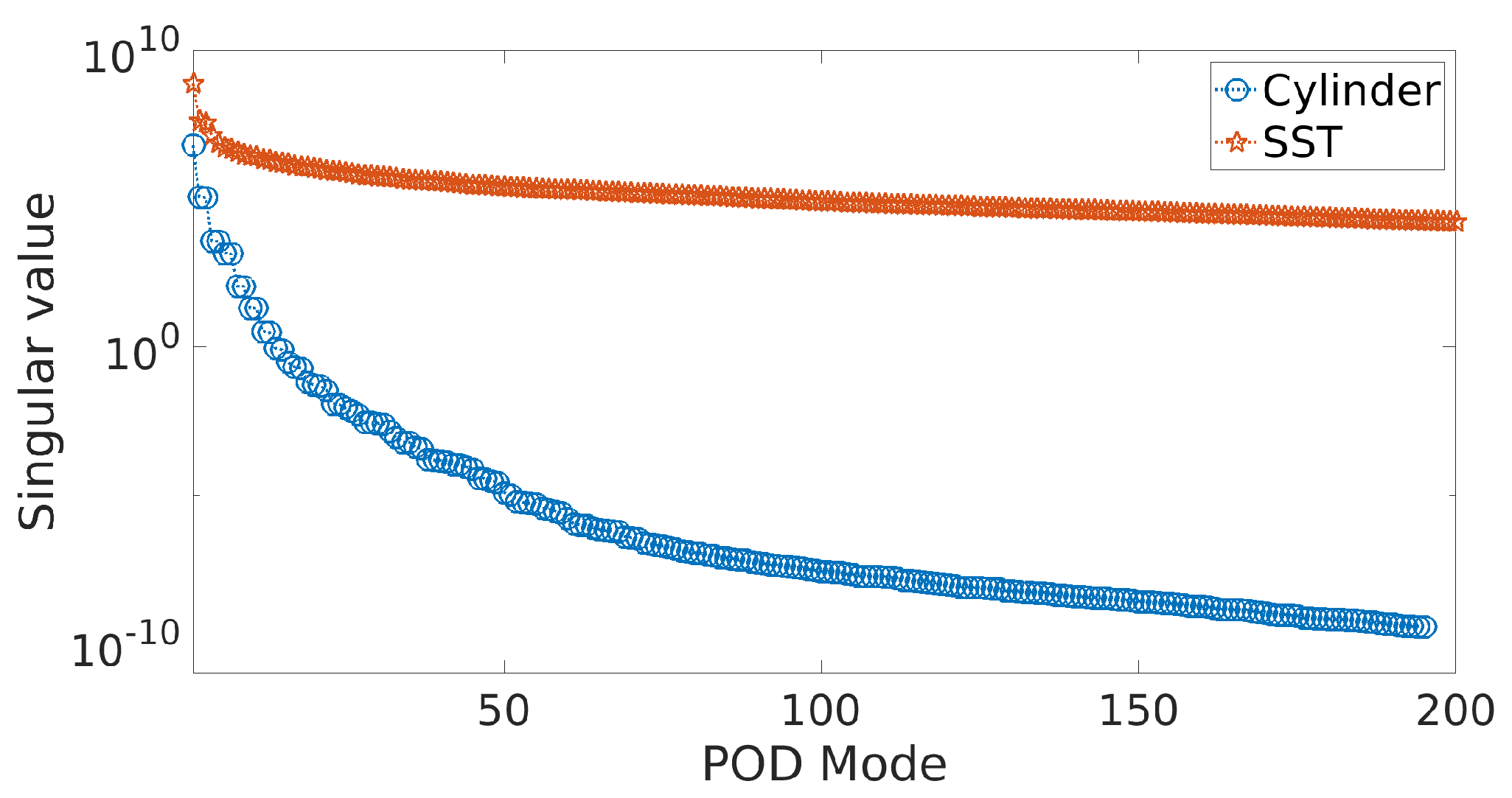
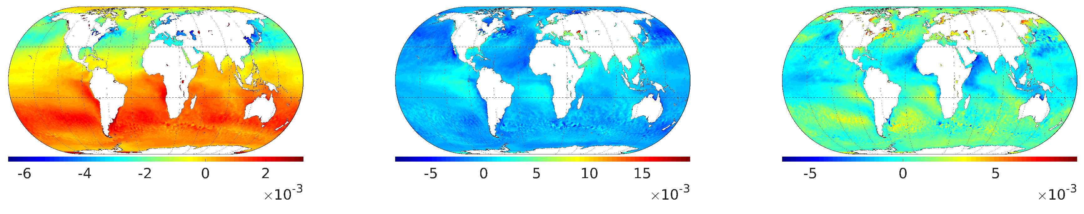
Figure 6.
Singular value spectrum of the data matrix for both the cylinder wake flow at and the sea surface temperature (SST) data.
Figure 6.
Singular value spectrum of the data matrix for both the cylinder wake flow at and the sea surface temperature (SST) data.
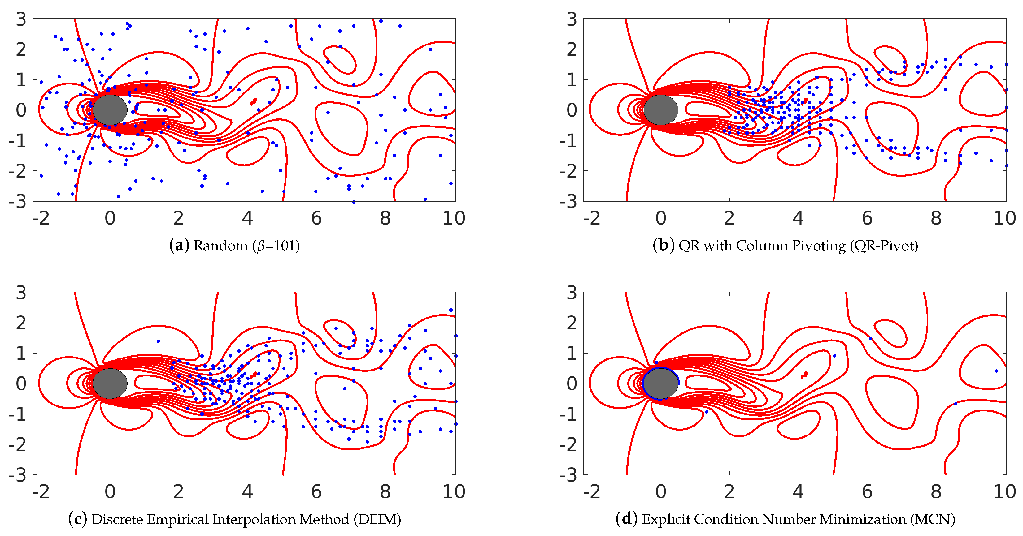
Figure 7.
Sensor locations generated using the different methods considered in this work including both random as well as smart algorithms for the cylinder wake flow (). These image show the most relevant 200 sensors, i.e., (), while (e) represents the grid distribution.
Figure 7.
Sensor locations generated using the different methods considered in this work including both random as well as smart algorithms for the cylinder wake flow (). These image show the most relevant 200 sensors, i.e., (), while (e) represents the grid distribution.
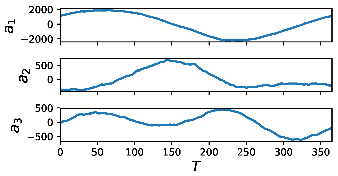
Figure 8.
Visualization of the first three POD modes (top left to right) and POD coefficients (bottom) for the sea surface temperature data.
Figure 8.
Visualization of the first three POD modes (top left to right) and POD coefficients (bottom) for the sea surface temperature data.
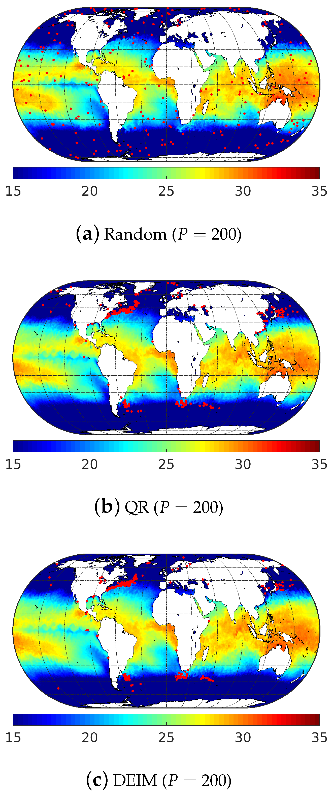
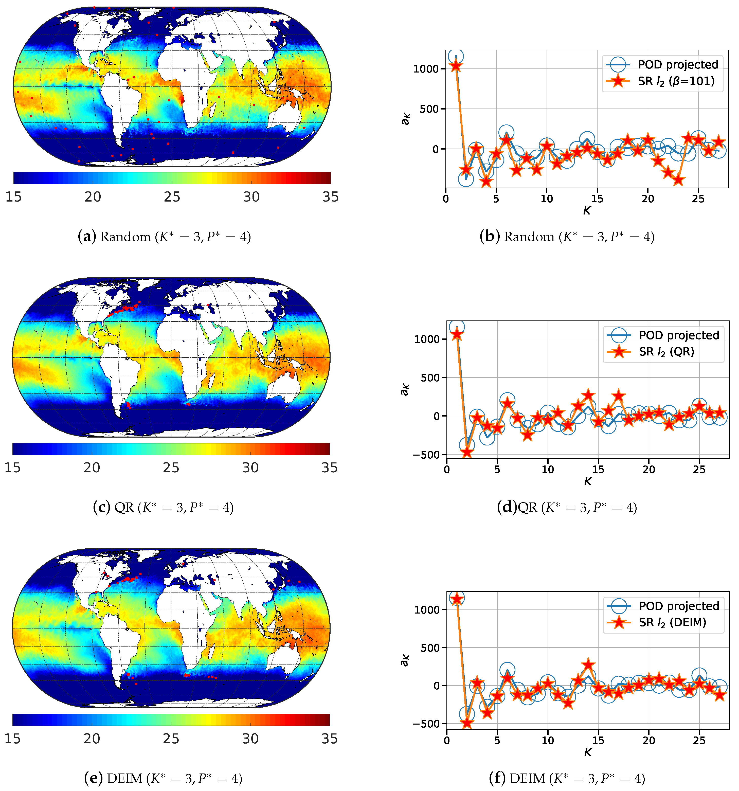
Figure 9.
Illustration of the 200 most relevant sensor locations (red dots) generated using: (a) random; (b) QR-pivot; and (c) DEIM methods for the sea surface temperature (in °C) data.
Figure 9.
Illustration of the 200 most relevant sensor locations (red dots) generated using: (a) random; (b) QR-pivot; and (c) DEIM methods for the sea surface temperature (in °C) data.
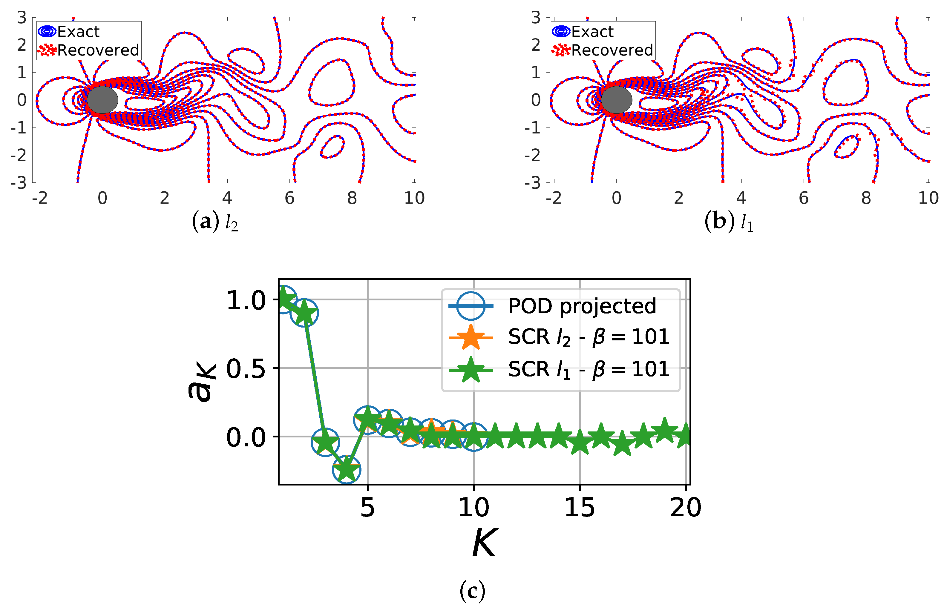
Figure 10.
Comparison of the sparse reconstruction using both and minimization methods for basis that is ordered in terms of energy content. The reconstructed and actual flowfields at are compared: (a) for ; and (b) for . The corresponding POD features from both methods are shown in (c).
Figure 10.
Comparison of the sparse reconstruction using both and minimization methods for basis that is ordered in terms of energy content. The reconstructed and actual flowfields at are compared: (a) for ; and (b) for . The corresponding POD features from both methods are shown in (c).
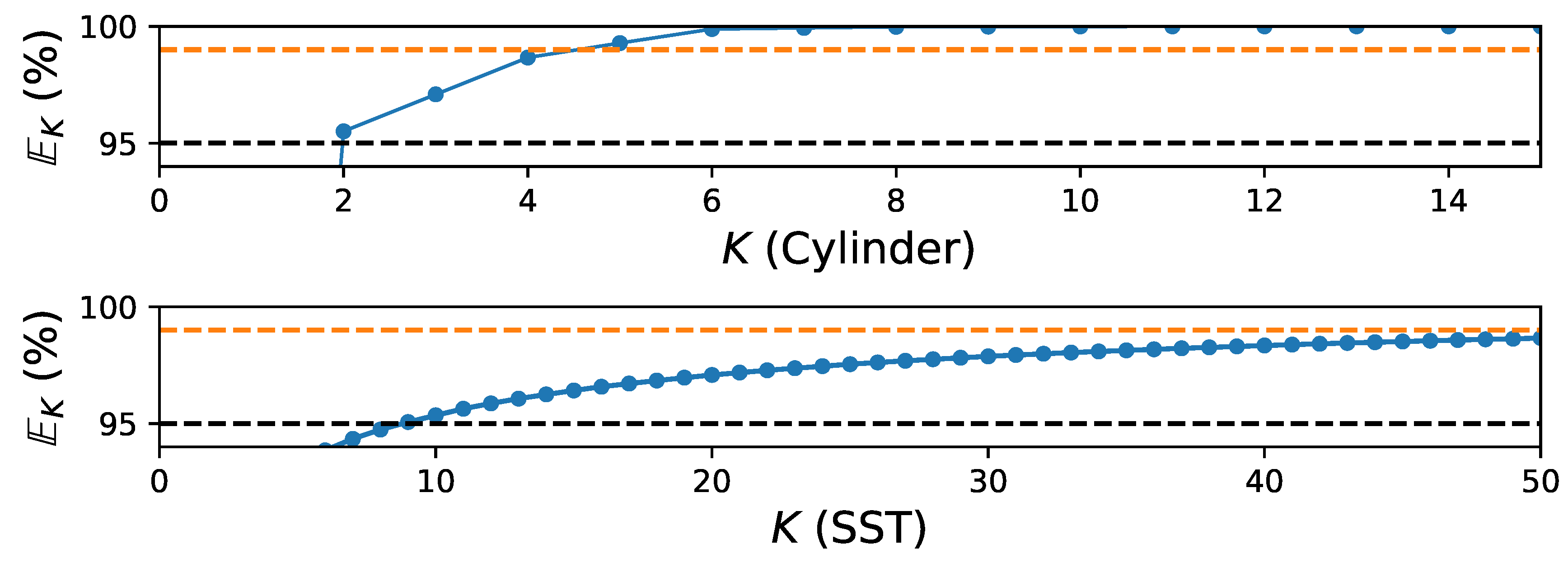
Figure 11.
Schematic shows the cumulative energy capture corresponding to different system dimension, K (i.e., the number of POD modes), for cylinder flow at (top) and sea surface temperature (SST) data (bottom).
Figure 11.
Schematic shows the cumulative energy capture corresponding to different system dimension, K (i.e., the number of POD modes), for cylinder flow at (top) and sea surface temperature (SST) data (bottom).
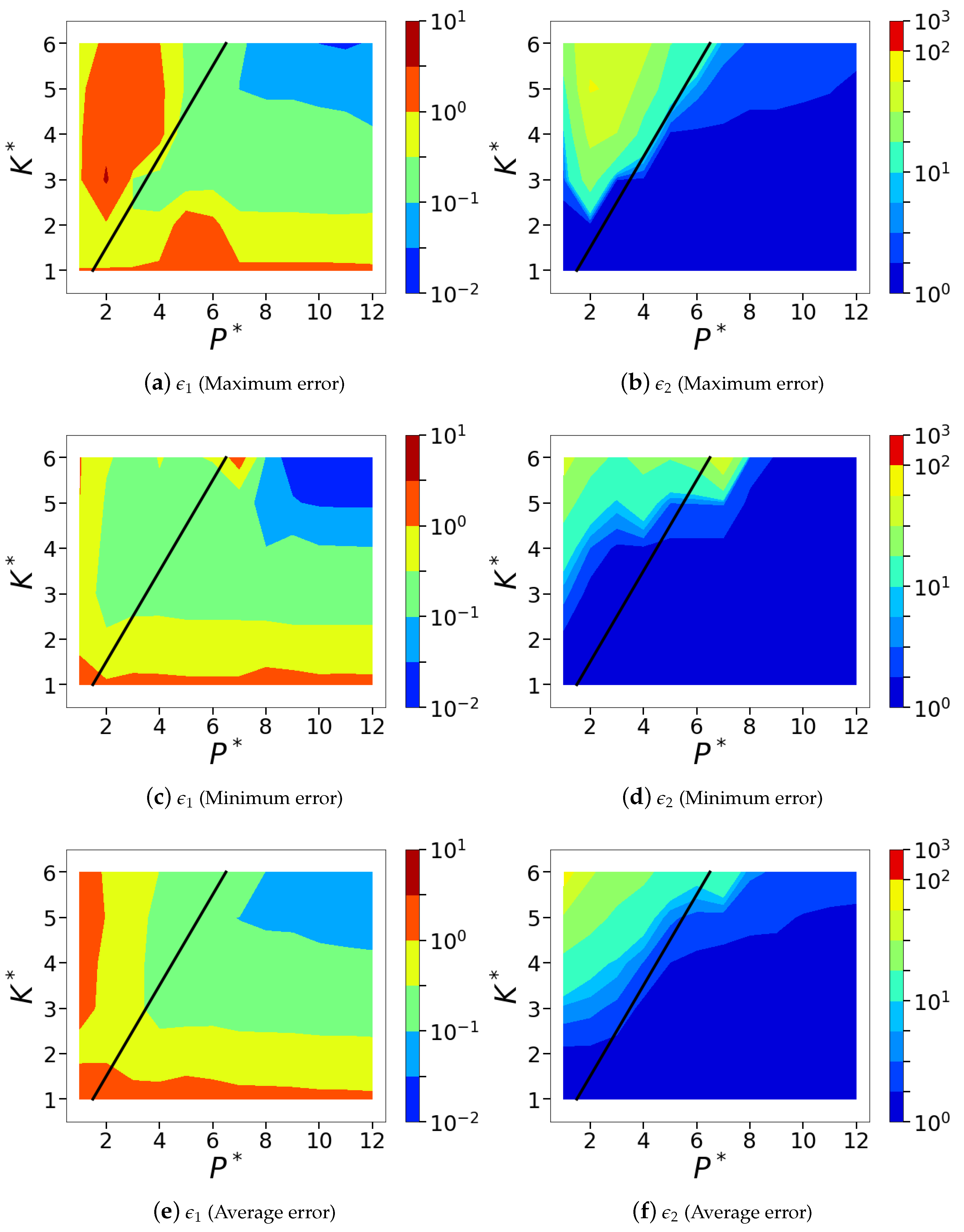
Figure 12.
Isocontours of the normalized mean squared POD-based sparse reconstruction errors ( norm) corresponding to the sensor placement with maximum and minimum errors from the chosen ensemble of random sensor arrangements. The average error across the entire ensemble of ten random sensor placements is also shown. Subfigures (a,c,e) show the normalized absolute error metric, and subfigures (b,d,f) show the normalized relative error metric, . Top row corresponds to the case with maximum error; middle row shows the case with minimum error and the bottom row shows the averaged error across different seeds.
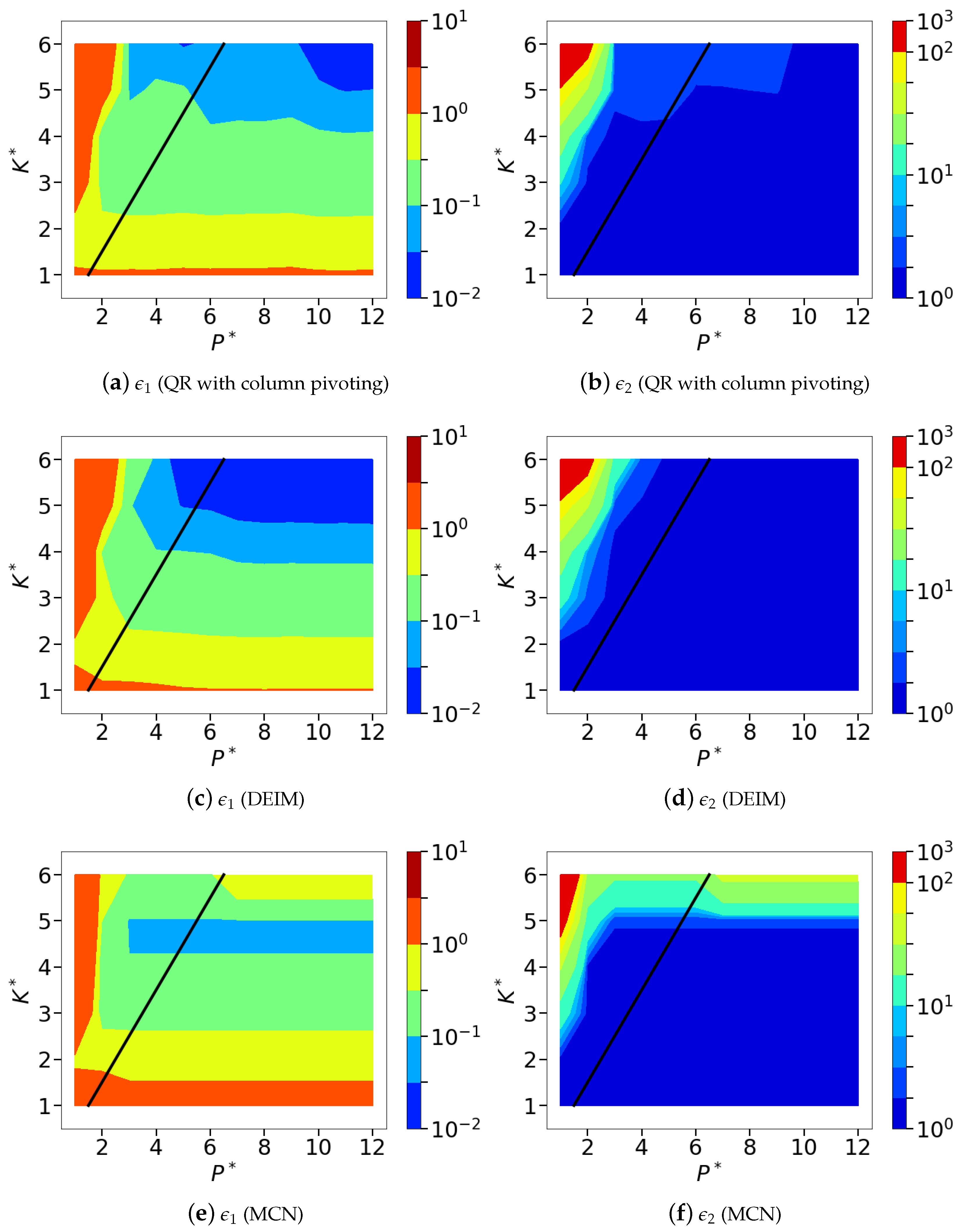
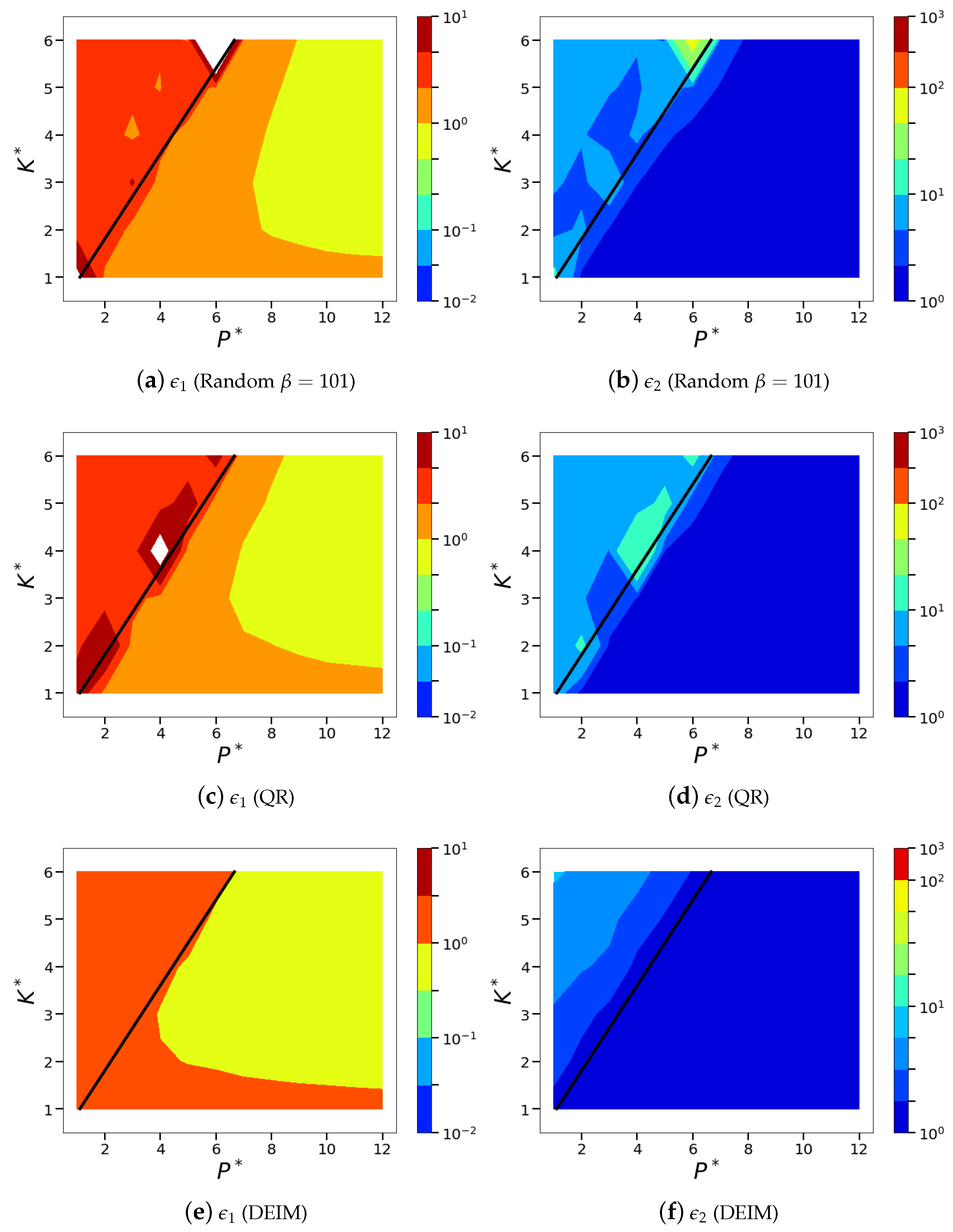
Figure 13.
Isocontours of the normalized mean squared POD-based sparse reconstruction errors ( norm) corresponding to the different greedy sensor placement methods, namely, QR with column pivoting (a,b), DEIM (c,d) and minimum condition number (e,f). Subfigures (a,c,e), show the normalized absolute error metric, and subfigures (b,d,f) show the normalized relative error metric, .
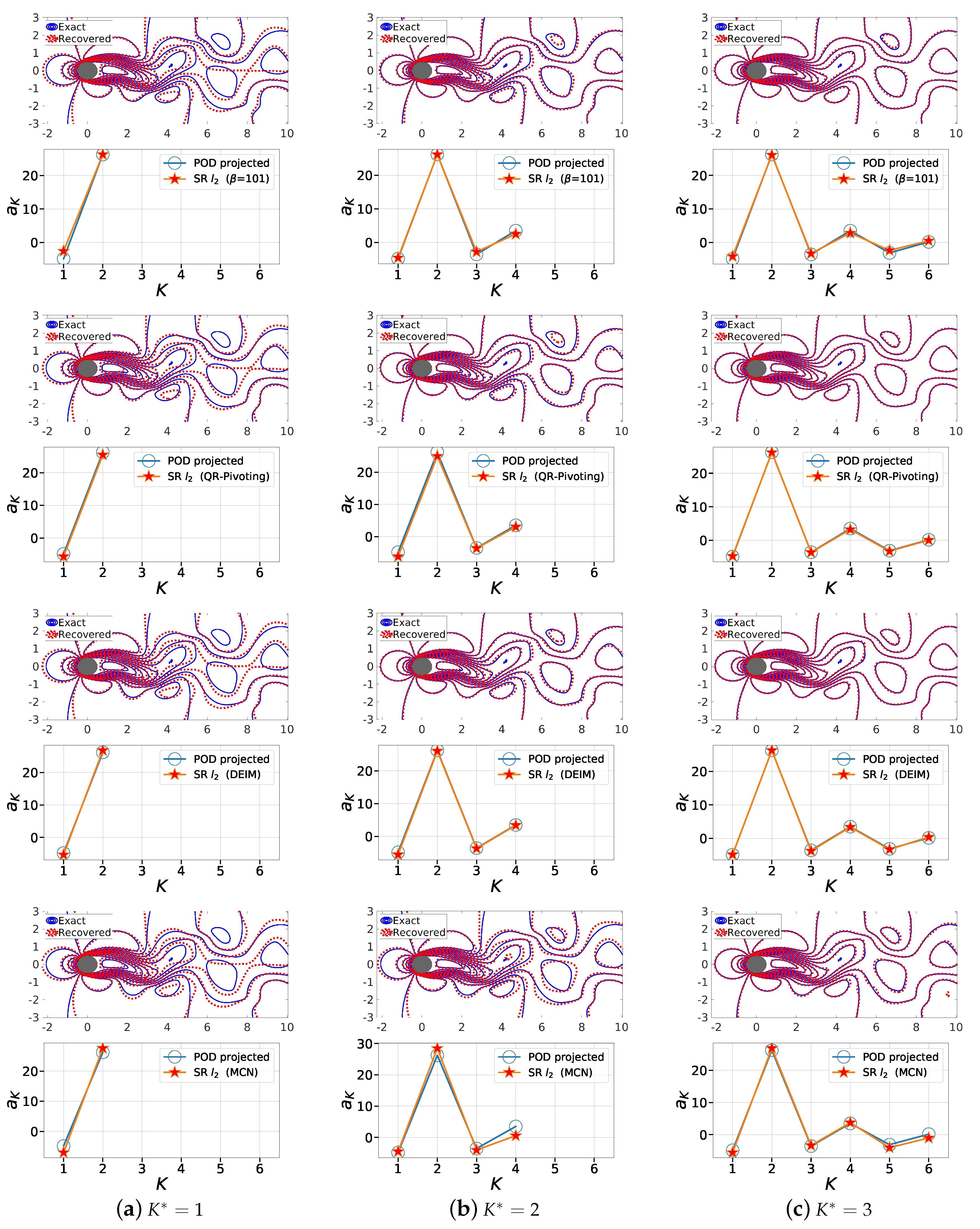
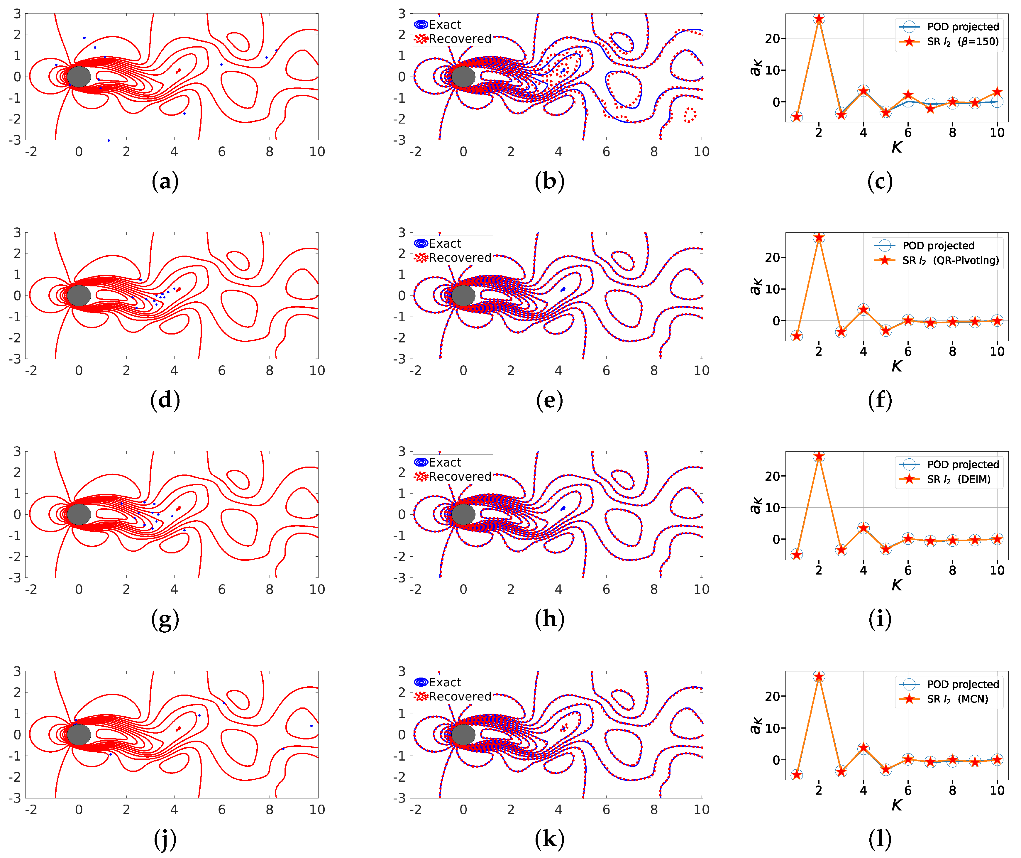
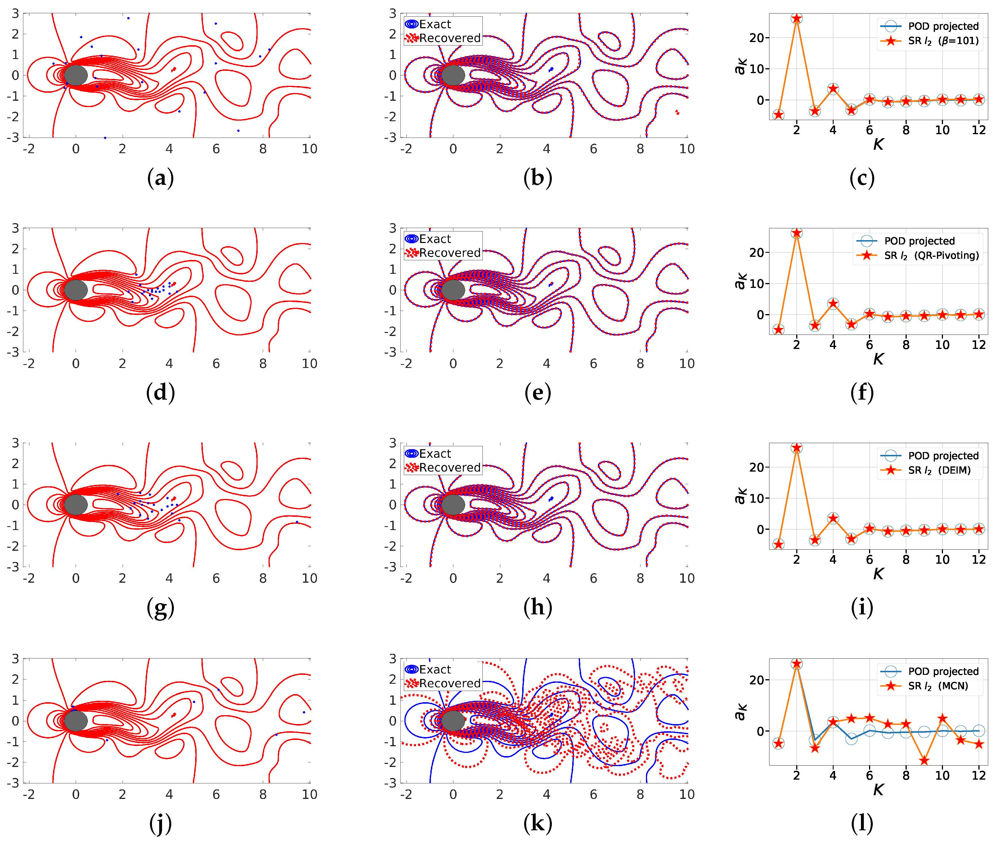
Figure 14.
First row (Random ), third row (QR-Pivot), fifth row (DEIM) and seventh (MCN) row: we show the line contour comparison of streamwise velocity between the actual CFD solution field (blue) and the POD-based SR reconstruction (red) for at and (a) , (b) , (c) . Second row (Random ), fourth row (QR with column pivoting), sixth row (DEIM) and eighth row (MCN) show the corresponding projected (full reconstruction) and sparse recovered coefficients a from the SR algorithm.
Figure 15.
Dissection of instantaneous snapshot reconstruction for a marginally oversampled case (). The figure shows the different sensor locations, namely random sensors with seed (a), QR factorization with column pivoting (b), DEIM (c) and minimum condition number (MCN) (d) along with the corresponding overlaid true and reconstructed solutions (b,e,h,k), and the recovered coefficients a (c,f,i,l) using POD-based SR for . The corresponding error quantifications for the different cases are as follows. First row: = and = 8.18. Second row: = and = 2.37. Third row: = and = 1.47. Fourth row: = and = 2.67.
Figure 16.
Dissection of instantaneous snapshot reconstruction for a highly oversampled case ( ). The figure shows the different sensor locations, namely random sensors with seed (a), QR factorization with column pivoting (b), DEIM (c) and minimum condition number (MCN) (d) along with the corresponding overlaid true and reconstructed solutions (b,e,h,k), and the recovered coefficients a (c,f,i,l) using POD-based SR for . The corresponding error quantifications for the above cases are as follows. First row: = and = 3.43. Second row: = and = 1.80. Third row: = and = 1.19. Fourth row: = and = 58.60.
Figure 17.
Isocontours of the normalized mean squared POD-based sparse reconstruction errors ( norm) of sea surface temperature data corresponding to the Random (a,b), QR (c,d) and DEIM (e,f) sensor placement methods. Subfigures (a,b,e) show the normalized absolute error metric, and subfigures (b,d,f) show the normalized relative error metric, .
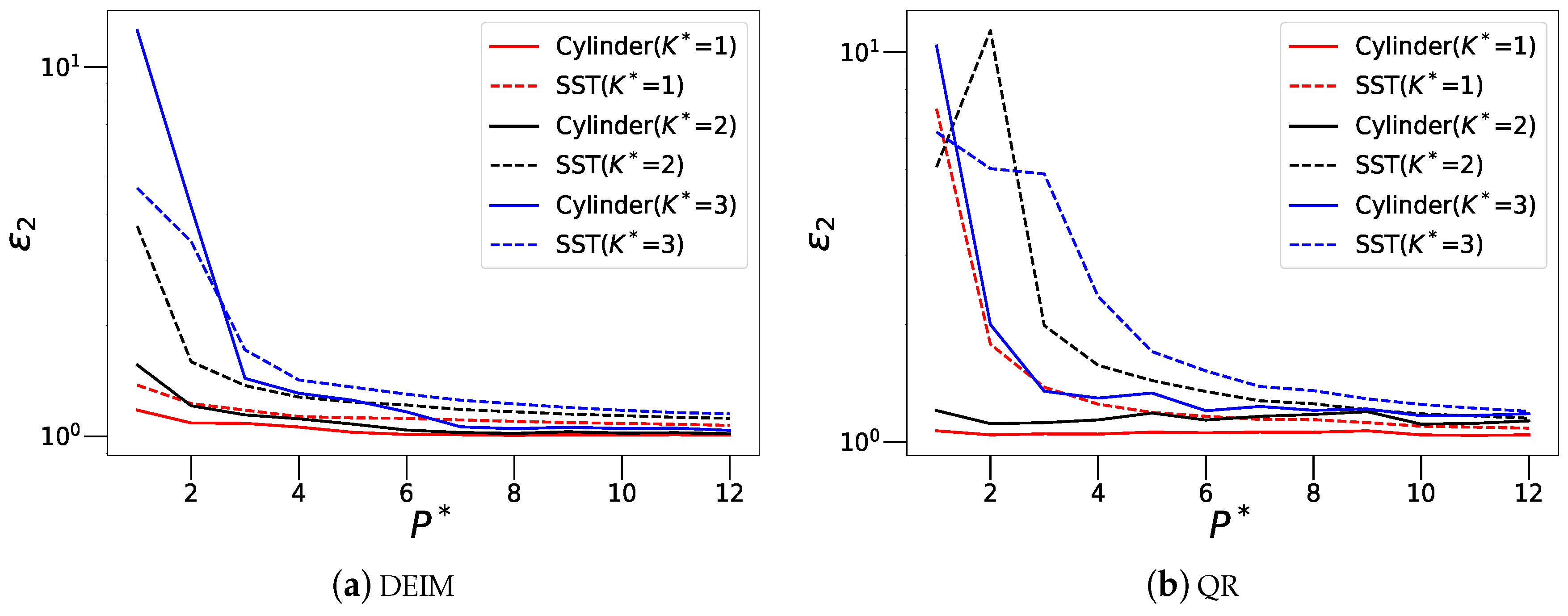
Figure 18.
Comparison of relative error () decrease with increasing sensor budget for both wake and SST data. The figure shows three curves for different values of for both DEIM (a) and QR-pivoting (b) based sensor placement.
Figure 18.
Comparison of relative error () decrease with increasing sensor budget for both wake and SST data. The figure shows three curves for different values of for both DEIM (a) and QR-pivoting (b) based sensor placement.
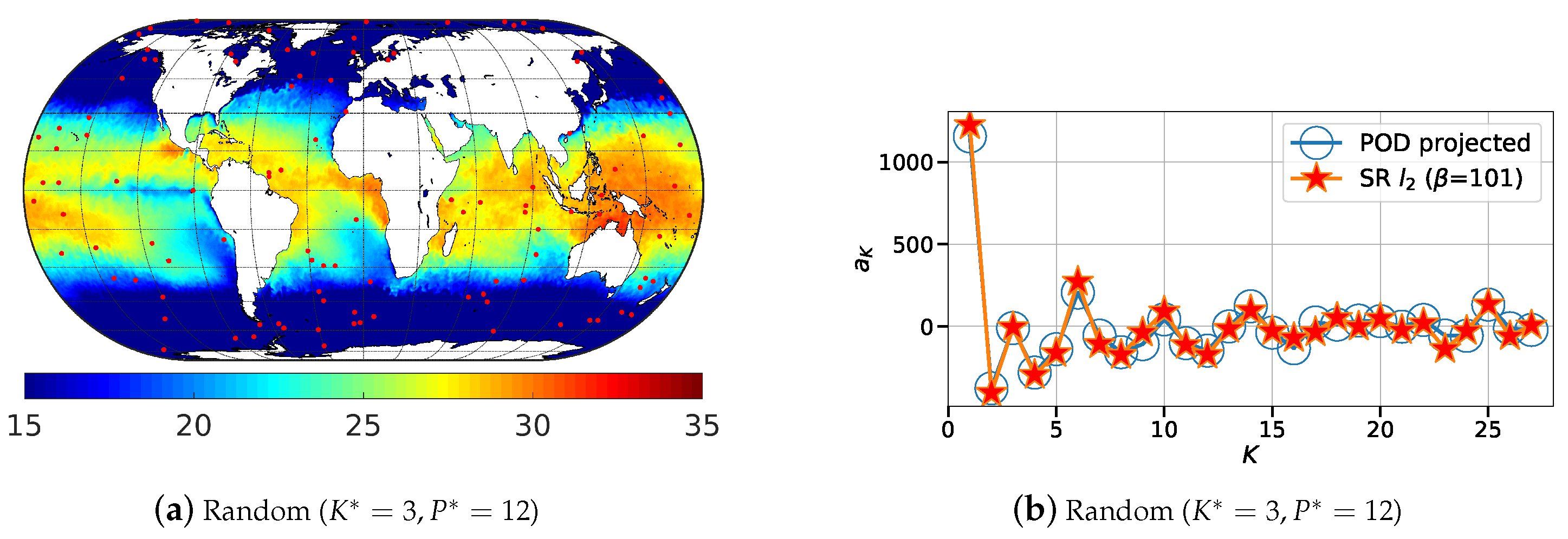
Figure 19.
Comparison of the sparse reconstruction using Random, QR and DEIM sensor placement method on instantaneous snapshot for a marginally oversampled case (). The left subfigures show the reconstructed solutions for different sensor placement methods namely, random placement (a), QR with column pivoting (c) and DEIM (e) whereas the corresponding reconstructed coefficients using POD-based SR are shown in subfigures (b,d,f). Red dots on the contour plots represent sensor locations.
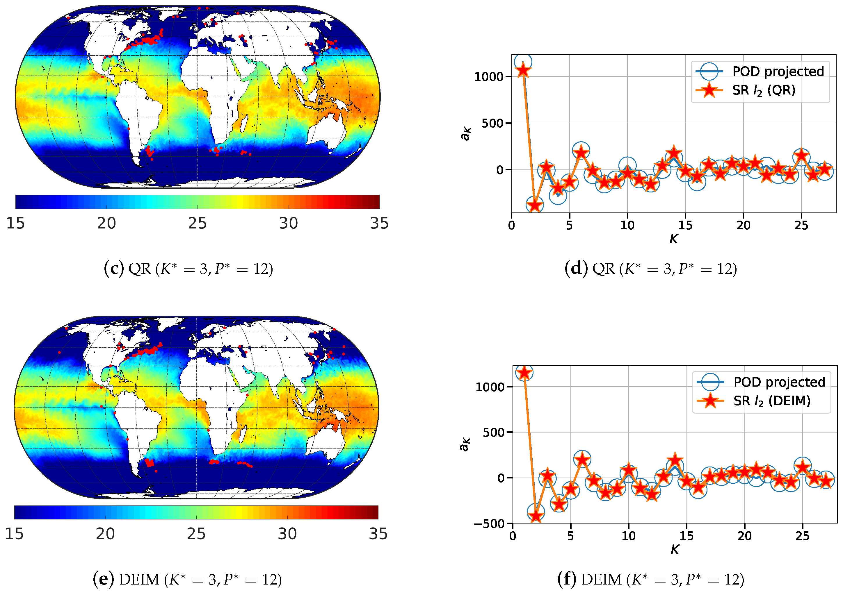
Figure 20.
Comparison of the sparse reconstruction using Random, QR and DEIM sensor placement method on instantaneous snapshot for a highly oversampled case (). The left subfigures show the reconstructed solutions for different sensor placement methods namely, random placement (a), QR with column pivoting (c) and DEIM (e) whereas the corresponding reconstructed coefficients using POD-based SR are shown in subfigures (b,d,f). Red dots on the contour plots represent sensor locations.
Table 1.
The choice of sparse reconstruction algorithm based on problem design using parameters P (sensor sparsity), K (targeted reconstruction sparsity) and (candidate basis dimension).
Table 1.
The choice of sparse reconstruction algorithm based on problem design using parameters P (sensor sparsity), K (targeted reconstruction sparsity) and (candidate basis dimension).
| Case | Relationship | Relationship | Algorithm | Reconstructed Dimension |
|---|
| 1 | | | least squares | K |
| 2 | | | min. norm recons. or | P |
| 3 | | | min. norm recons. | K |
Table 2.
Problem design for comparison.
Table 2.
Problem design for comparison.
| Method | | K | P | | |
|---|
| 100 | 10 | 40 | 10 | 101 |
| 100 | 10 | 40 | 20 | 101 |
Table 3.
Sparse reconstruction performance quantification for different sensor location selection method for periodic cylinder flows at . is the SR error normalized by the exact reconstruction error corresponding to a dimension of . is the SR error normalized by the exact reconstruction error corresponding to a dimension of K.
| Method | K | P | | | | | | |
|---|
| Random () | 2 | 20 | 1.0 | 10.0 | 2.548 | 2.306 | 1.08 | 1.08 |
| 4 | 20 | 2.0 | 10.0 | 2.548 | 3.247 | | 1.23 |
| 6 | 20 | 3.0 | 10.0 | 2.548 | 4.186 | | 1.96 |
| QR-Pivoting | 2 | 20 | 1.0 | 10.0 | 2.520 | 3.794 | 1.04 | 1.04 |
| 4 | 20 | 2.0 | 10.0 | 3.917 | 3.794 | | 1.11 |
| 6 | 20 | 3.0 | 10.0 | 3.917 | 4.506 | | 1.16 |
| DEIM | 2 | 20 | 1.0 | 10.0 | 2.323 | 3.720 | 1.00 | 1.00 |
| 4 | 20 | 2.0 | 10.0 | 3.685 | 3.867 | | 1.02 |
| 6 | 20 | 3.0 | 10.0 | 3.685 | 4.562 | | 1.05 |
| MCN | 2 | 20 | 1.0 | 10.0 | 1.090 | 2.213 | 1.15 | 1.15 |
| 4 | 20 | 2.0 | 10.0 | 1.476 | 3.502 | | 1.59 |
| 6 | 20 | 3.0 | 10.0 | 1.476 | 3.725 | | 1.71 |


