Article

Added Mass Effects on a Francis Turbine Runner with Attached Blade Cavitation

1
WinGD Ltd., Schützenstrasse 1-3, 8401 Winterthur, Switzerland
2
Department of Fluid Mechanics, Universitat Politècnica de Catalunya, Av. Diagonal 647, 08028 Barcelona, Spain
*
Author to whom correspondence should be addressed.
Fluids 2019, 4(2), 107; https://doi.org/10.3390/fluids4020107
Submission received: 18 May 2019 / Revised: 4 June 2019 / Accepted: 5 June 2019 / Published: 11 June 2019
(This article belongs to the Special Issue Turbomachinery Flow Analysis)

Abstract

:
To have a safe structural design, an analysis of the dynamic behavior of a Francis turbine runner with consideration of the added mass effects of surrounding water is necessary during design phase. Both in design and at off-design operations, large-scale forms of attached cavitation may appear on runner blades and can change the added mass effects of the surrounding fluid in relation to a single water domain. Consequently, a numerical investigation of the modal response of a Francis runner has been carried out by reproducing the presence of various sizes of leading edge cavitation (LEC) and trailing edge cavitation (TEC). The fluid–structure interaction problem has been solved by means of an acoustic-structural coupling method. The calculated added mass effects with cavitation have been compared with those corresponding to the pure water condition without cavitation. Firstly, a single blade has been investigated to evaluate the level of significance for the proposed cavity shapes and dimensions. Afterwards, based on the results obtained, the complete runner structure has been considered, factoring in similar cavity shapes and locations. The results prove that significant added mass effects are induced on the entire runner by the attached cavitation that increase the natural frequencies of the first modes. Moreover, the added mass effects increase with cavity size and amplitude of blade deformation below the cavity.

1. Introduction

Hydropower, a clean and renewable energy resource, has been developed worldwide for the economic growth and improvement of people’s living standards. It has also been frequently used to improve the stability and safety of smart power grids.
Depending on the water head available at hydropower plants, various types of hydraulic turbines such as Francis, Kaplan and Pelton can be selected to maximize energy conversion efficiency. Francis turbines, which combine radial and axial flows, are the most common type in use nowadays because they can operate in a quite wide water head range. In order to meet the ever-changing power requirements of the electrical grid, Francis turbines have to work under various operating conditions from no-load to maximum load. At a given water head, the power output of Francis turbines can be controlled by adjusting the flow discharge with the wicket gate opening. However, this changes the flow pattern dramatically within the runner blade channels. Furthermore, extreme hydrodynamic conditions, provoking strong pressure reductions, are found by the irregular flow inside the runner channels when the turbine operates both at low part loads and over loads, below and above the best efficiency point, respectively. Consequently, both at off-design and at design operation conditions, two-phase flows with large scale cavitation forms may occur inside the Francis runners [1]. Cavitation is the condition when local pressure reaches vapor pressure, causing vapor cavities to form and grow within a liquid. Within flowing water, cavitation can take the form of bubbles, macro-cavities that develop and attach to the solid walls or vortices. Moreover, the plant cavitation number or Thoma number [2] can change due to unavoidable variations of the tail water level during operation at a given condition, which can increase the risk of cavitation.
Cavitation phenomena in Francis runners have been well investigated with model tests and site measurement campaigns [
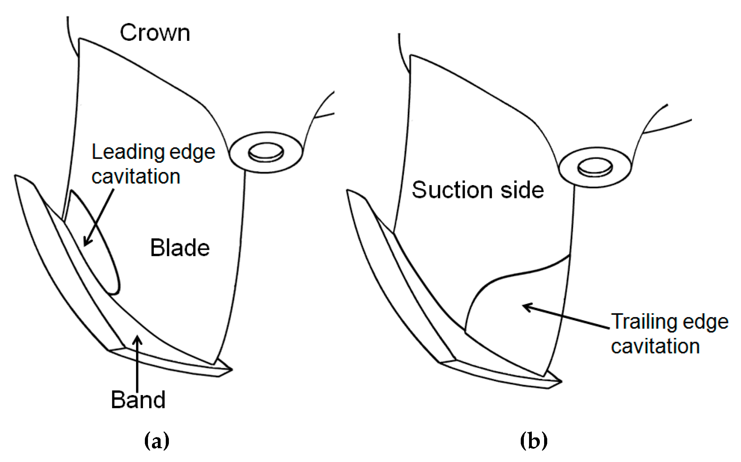
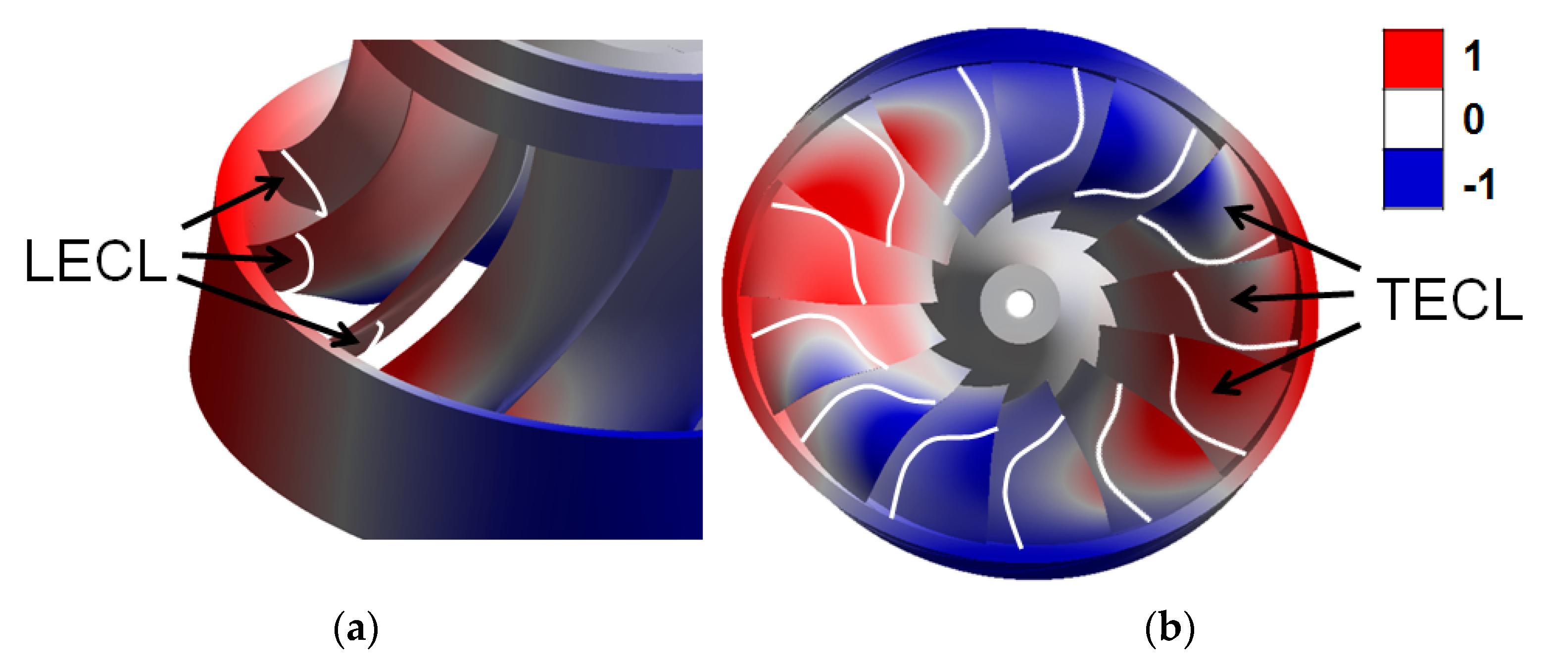
3]. The typical blade-attached forms of cavitation in a Francis runner are leading edge cavitation (LEC) and trailing edge cavitation (TEC). LEC appears on the suction side of runner blades due to operation at a higher head than the machine design head when the incidence angle of the inlet flow is positive and largely deviated from the design value. TEC appears as separated bubbles attached to the blade suction side, located near the mid-chord next to the trailing edge. These travelling bubbles appear due to a low plant cavitation number reaching their maximum when the machine operates in overload condition with the highest flow rate.
In order to avoid damages provoked by vibration resonances and material fatigues due to hydraulic excitations [4,5], the structural behavior of the turbine runner has to be carefully investigated during the design phase. Extensive research has been carried out to measure and characterize the vibrations and dynamic stresses induced by pressure fluctuations in Francis turbines [6,7] and pump-turbines [8,9]. Many research works have been carried out to predict the dynamic behavior of Francis runners in air and still water based on both measurements and simulations in reduced scale models of Francis runners [10,11] and pump-turbines [12,13]. The final objective is to identify the natural frequencies and the damping ratios of the runner, taking into account the added mass and damping of the surrounding water, because it has been demonstrated that these effects can considerably affect the results [14]. Moreover, additional boundary conditions such as the proximity of walls can also influence the added mass effects, which have been investigated from simple structures like disks [15] to actual prototype structures [16,17,18].
However, the possible effect of cavitation inside hydraulic turbines has not been sufficiently addressed, and only one recent work has numerically investigated the possibility that inter-blade cavitation vortices are responsible for multiple fractures that have appeared on the trailing edge of full-scale Francis runner blades [19]. For example, the added mass effects of the presence of attached cavitation on the runner blades have not been calculated yet. Under this condition, a significant region of the surrounding fluid in contact with the structure is occupied by vapor instead of water, meaning that the density is locally reduced. In particular, only limited research has been performed on hydrofoil to investigate the added mass effects under partial cavitation, and the significance of this [20,21] has not been demonstrated in comparison with the no cavitation condition. However, hydrofoil is only a very simple structure compared with the complex Francis runner. Therefore, it is necessary to consider the geometry of an actual Francis runner with all its complexity.
Consequently, a Francis runner with 13 blades and a diameter of 2.12 m (Figure 1) has been selected to carry out the structural behavior analysis by numerical simulation. The objective of the current work is to quantify the influence that the presence of cavitation might have on the modal behavior of the runner. For that, both LEC and TEC of different sizes have been considered, and the added mass effects have been compared with those corresponding to the pure water condition without cavitation. A review of the numerical results of cavitation in Francis turbine runners [22] and the visual observations from reduced scale models [23] and full-scale Francis prototypes [24] has permitted us to determine the most probable locations and sizes of cavitation, as shown in Figure 2. First of all, a single blade has been investigated to evaluate the level of significance for the proposed cavity shapes and dimensions. Furthermore, based on the results obtained, the complete runner structure has been considered with similar cavity shapes and locations on all the blades.

2. Added Mass and Frequency Reduction Ratio

The concept of added mass was developed by several authors like Lamb [25] and Milne-Thomson [26] for the two-dimensional case of a circular cylinder of radius a moving forward in liquid with velocity U and density ρ . In this case, the kinetic energy per unit thickness of the fluid is given by
T f = 1 2 π ρ a 2 U 2
Let M = π ρ a 2 , then M is the mass of the liquid (per unit thickness) displaced by the cylinder.
If M is the mass of the cylinder (per unit thickness), the total kinetic energy of the fluid and the cylinder is
T = 1 2 ( M + M ) U 2
Let F be the external force in the direction of motion of the cylinder necessary to maintain the motion. Then, the rate at which F does work must be equal to the rate of increase of the total kinetic energy, and therefore
F U = d T d t = ( M + M ) U d U d t
F M d U d t = M d U d t
Thus, the cylinder experiences a resistance to its motion due to the presence of the liquid, and the amount of resistance per unit thickness equals
M d U d t
Therefore, the presence of the liquid effectively increases the mass of a moving circular cylinder from M to M + M that is called the “virtual mass” of the liquid displaced. The virtual mass is obtained by adding the mass M and the added mass or hydrodynamic mass M .
As analogously explained by Brennen [27], whenever acceleration is imposed on a fluid flow by acceleration of a body, additional fluid forces will act on the surfaces in contact with the fluid due to the added mass. These inertial fluid forces can be of considerable importance in many engineering problems if a structure is submerged in water. For example, the added mass of the cylinder with potential flow for rectilinear motion is equal to the mass of the fluid displaced by the cylinder, as previously expressed in Equation (1). However, this should be regarded as coincidental, because there is no general correlation between the added mass and displaced fluid mass. Furthermore, in general, the value of the added mass depends on the direction of acceleration. Therefore, the added mass must be characterized with the added mass matrix.
The added mass matrix provides a method of expressing the relationship between the six force components imposed on the body by the inertial effects of the fluid due to the three translation accelerations in three perpendicular directions and the three angular accelerations. Unfortunately for complex geometry, the added mass matrix cannot be theoretically predicted with sufficient accuracy.
If a solid body is vibrated, the general equation of a motion is
M s x ¨ + C s x ˙ + K s x = F
where Ms is the mass, Cs is the damping, Ks is the stiffness, F is the force applied to the body and x , x ˙ and x ¨ are displacement, velocity and acceleration, respectively. When this body is surrounded by a still fluid then the equation of motion is
( M s + M f ) x ¨ + ( C s + C f ) x ˙ + ( K s + K f ) x = F
where Mf is the added mass, Cf is the added damping and Kf is the added stiffness.
When the body is considered to be lightly damped to vibrate in-vacuum conditions without any surrounding fluid, the natural frequency of a mode of vibration is expressed as
f v a c u u m = k m
where k and m are the modal stiffness and modal mass, respectively. However, its dynamic response is significantly changed when it is submerged in a fluid with high density, such as water. The added modal mass, mf, then reduces the new natural frequency to
f f = k m + m f
The frequency reduction ratio (FRR) of a vibration mode can be calculated relative to in-vacuum conditions as expressed with
δ f = 1 f f f v a c u u m = 1 1 1 + m f m

3. Acoustic Fluid–Structural Coupling Method and Numerical Model

The acoustic fluid–structural coupling method (AFSCM) is commonly used to calculate the added mass effects of fluid on structures submerged in dense fluids like water. In our study, we used the finite element analysis tool available in ANSYS Mechanical, which takes into account the fluid–structure interaction phenomena, as described in [28].
Using the finite element method (FEM), the structural dynamic equilibrium equation is expressed as
M s u ¨ + C s u ˙ + K s u = f s ( t )
where Ms, Cs and Ks are the structure mass, damping and stiffness matrices, respectively; u, u ˙ , u ¨ are nodal displacement, velocity and acceleration vectors, respectively; fs(t) represents the externally applied force vector and t is time.
With consideration of the acoustic fluid pressure acting at the interface, Equation (11) can be described as
M s u ¨ + C s u ˙ + K s u = f s ( t ) + f f s ( t )
where ffs(t) = −Kfsp is the acoustic fluid pressure load vector at the interface, Kfs is the equivalent coupling stiffness matrix and p is the acoustic pressure vector.
In AFSCM, it is assumed that the fluid is compressible (density changes due to pressure variations) and that there is no mean flow of the fluid. To describe the fluid effect on the submerged structures, the discretized Helmholtz acoustic equation is adopted as
M f p ¨ + C f p ˙ + K f p = f s f ( t )
where Mf, Cf and Kf are the acoustic fluid equivalent mass, damping and stiffness matrices, respectively, and fsf(t) = −Mfs u ¨ is the fluid load produced by the structure displacement at the interface and Mfs is the equivalent coupling mass matrix.
Finally, the complete finite element discretized equations with assembled form expressed in Equation (14) can be used to solve acoustic fluid–structural coupling problems by considering Equations (12) and (13) simultaneously:
[ M s 0 M f s M f ] { u ¨ p ¨ } + [ C s 0 0 C f ] { u ˙ p ˙ } + [ K s K f s 0 K f ] { u p } = { f s ( t ) 0 }
Several works devoted to investigating the modal behavior and dynamic responses of hydraulic turbine runners both in air and water can be found in the literature based on FEM and AFSCM [4,5,6,7,8,9,10,11,12,13,14,15]. In all cases, the numerical results have shown a good agreement with the corresponding measured ones, which fully validates the feasibility of FEM and AFSCM for the current study.
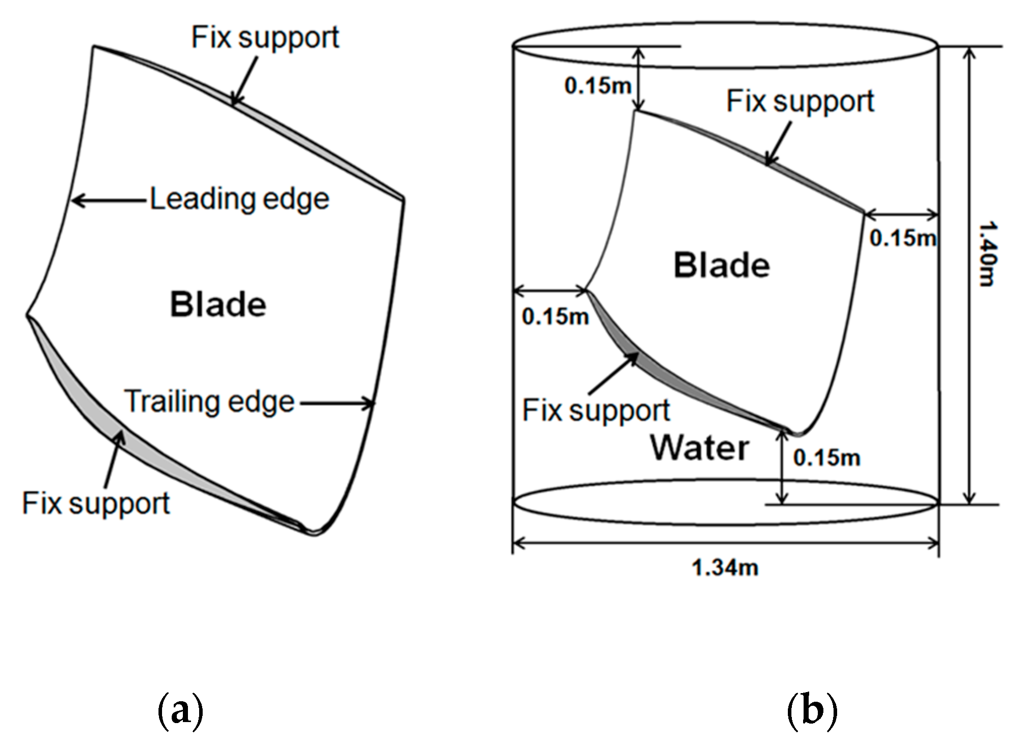
The single blade and the whole runner structure domains are built with high order tetrahedral structural elements that are suitable for modelling complex geometries. The fluid domains comprising the cavities and surrounding water have been meshed with tetrahedral acoustic elements, which are also typically used to solve fluid–structure coupling problems.
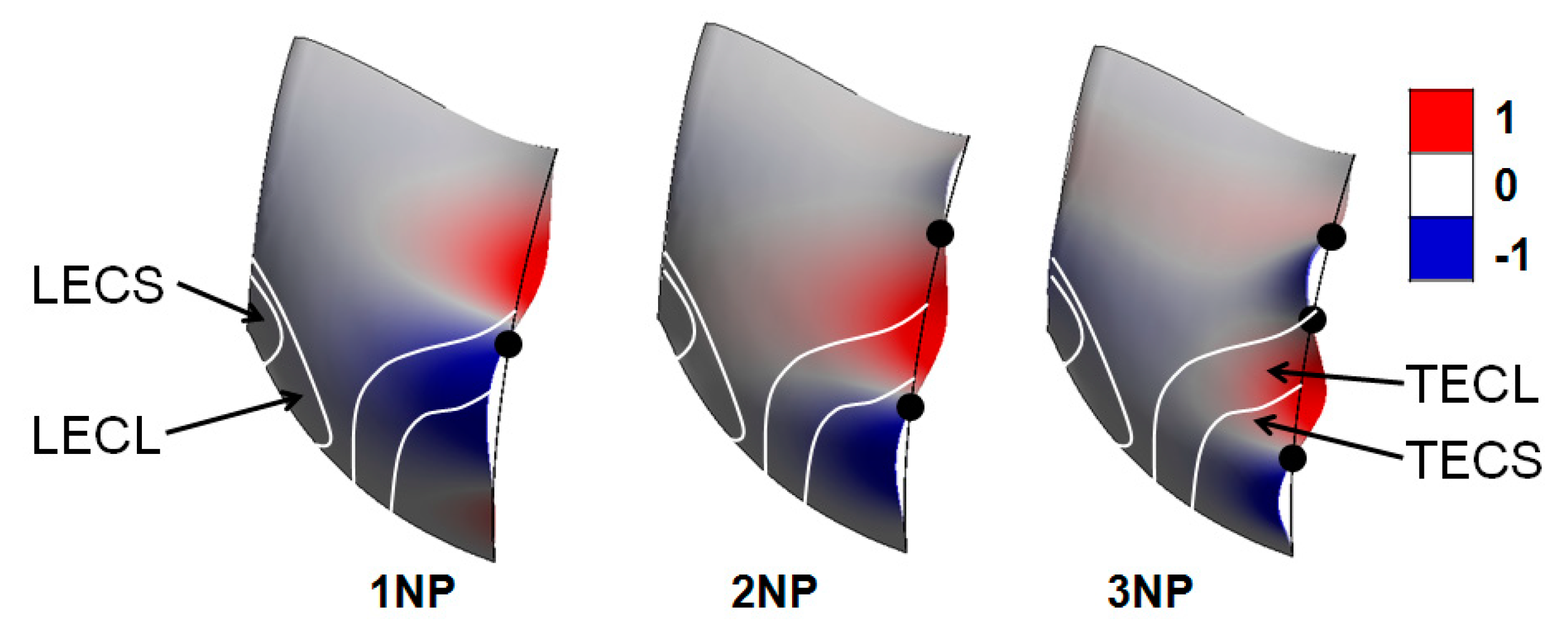
The proposed attached cavities with different dimensions and locations are modelled on the suction side of the runner blade (Figure 2). The thickness of attached cavities is assumed to be 0.0225 m, which is three times the blade trailing edge thickness.
The dimensions of the attached cavities have been calculated relative to the surface of the blade suction side in percentage and presented as the cavity to blade surface ratio (CSR), which is defined by
CSRCavity = 100 × SCavity/SSuction_side
where SCavity is the area of the cavity, and SSuction_side is the area of the blade suction side. These results are listed in Table 1, where LECS and LECL indicate small (S) and large (L) sizes of leading edge cavitation, respectively, and TECS and TECL indicate small (S) and large (L) sizes of trailing edge cavitation, respectively.
To guarantee the accuracy and convergence of the numerical model, results sensitivity to mesh size and density was analyzed based on previous experience first [9]. For that, three meshes with increasing numbers of elements were constructed for both the single blade and entire turbine runner, as shown at the top of Figure 3. The graphs present the evolutions of the predicted natural frequencies when the element number increases, as well as how they converge towards constant values. The meshes providing the results marked with dashed line boxes were finally selected to perform the simulations. The corresponding numbers of elements for the structures and fluid domains are indicated in Table 2.
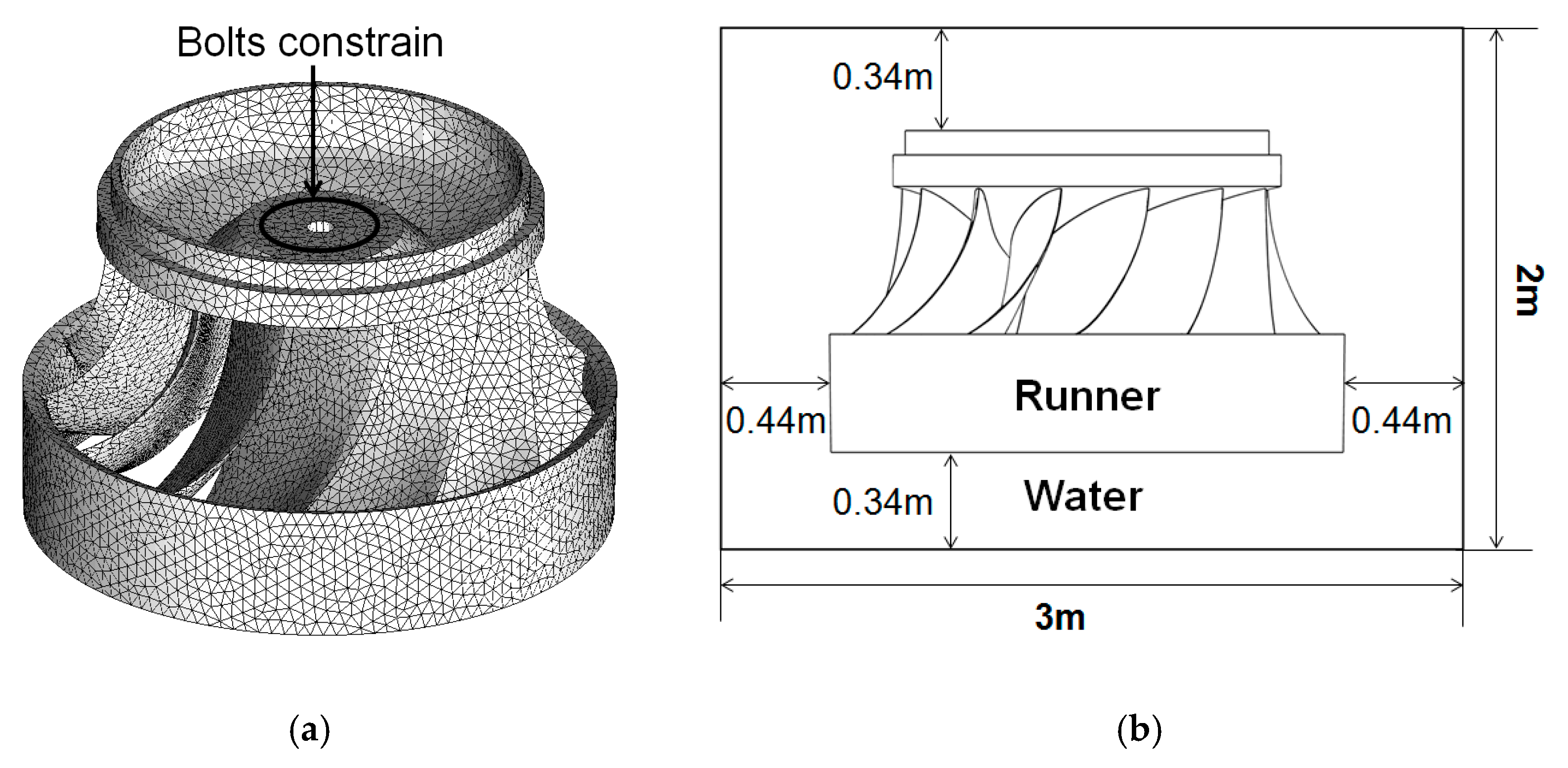
Moreover, based on the results obtained by Rodriguez et al. [10] with a similar runner geometry, and in order to have a sufficiently large fluid domain, the surfaces of the fluid domain where located at a distance around 1/3 to 1/4 of the runner height relative to the runner outer surfaces as shown at the right of Figure 4. And the fluid domain for the single blade is shown at the left of Figure 4.
The material properties of the cavitation domains are the corresponding ones to pure saturated vapor, assuming a vapor volume fraction of 1. As a summary, the material properties of the structure and both fluids, water and vapor, used in the numerical calculations are tabulated in Table 3.
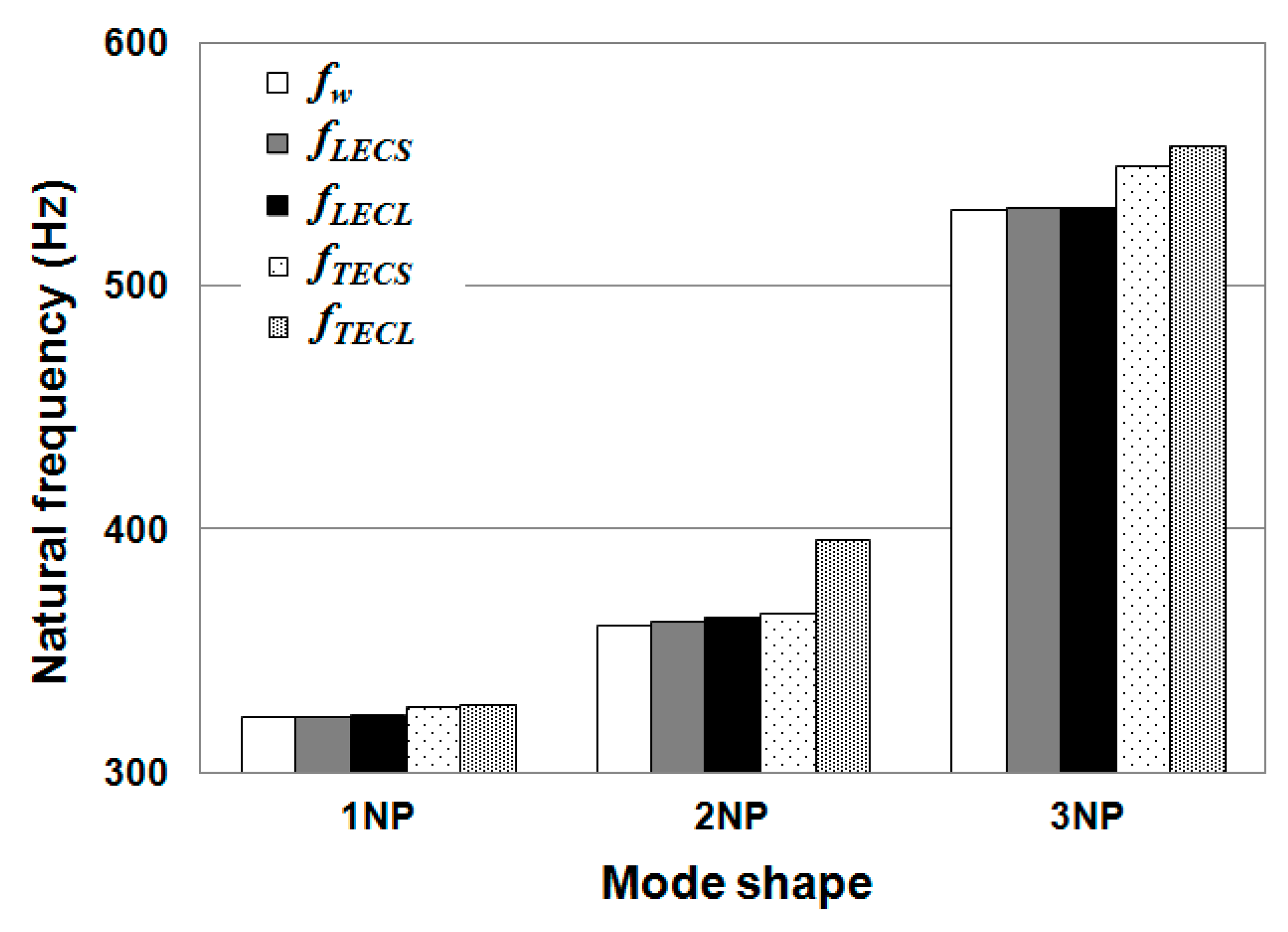
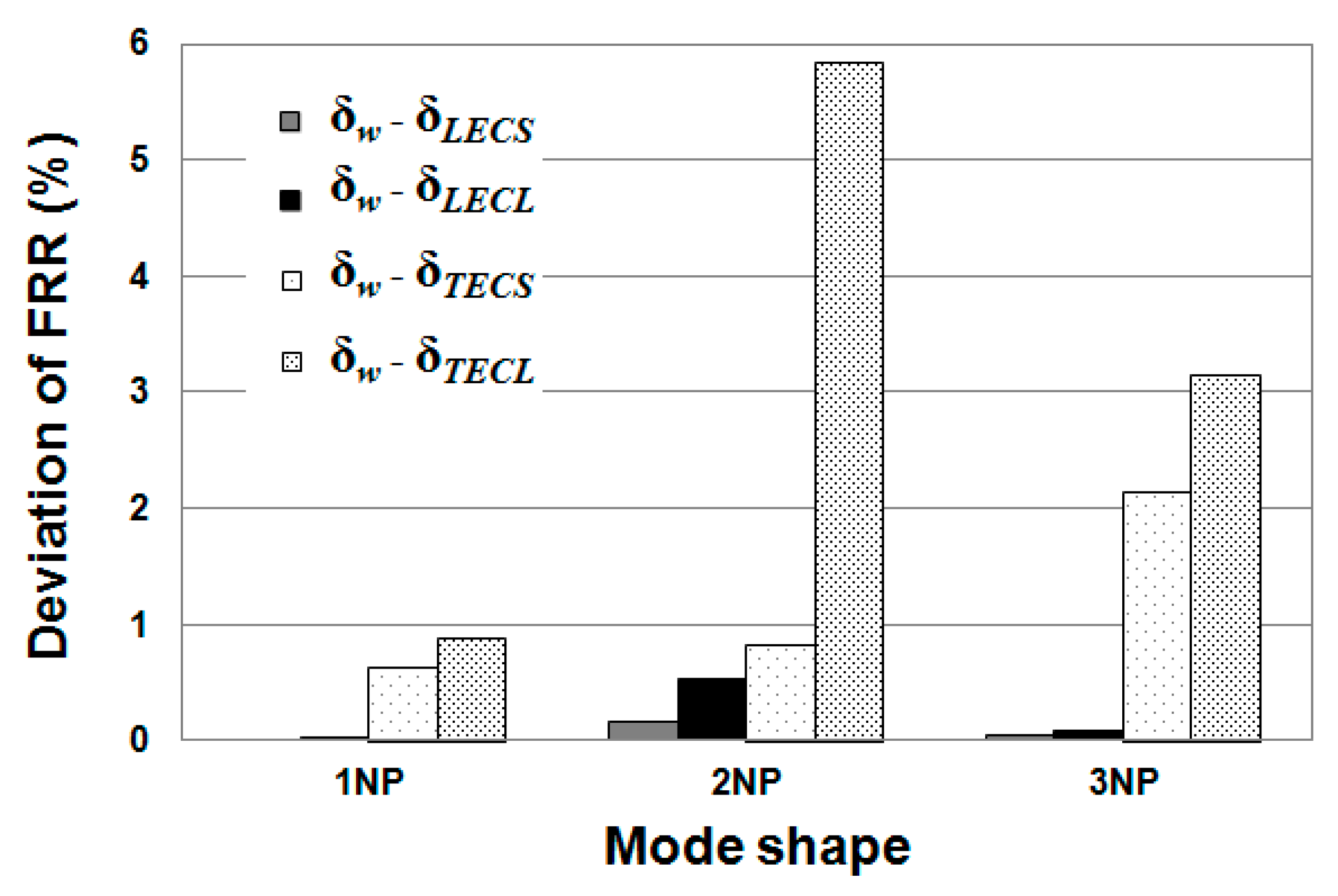
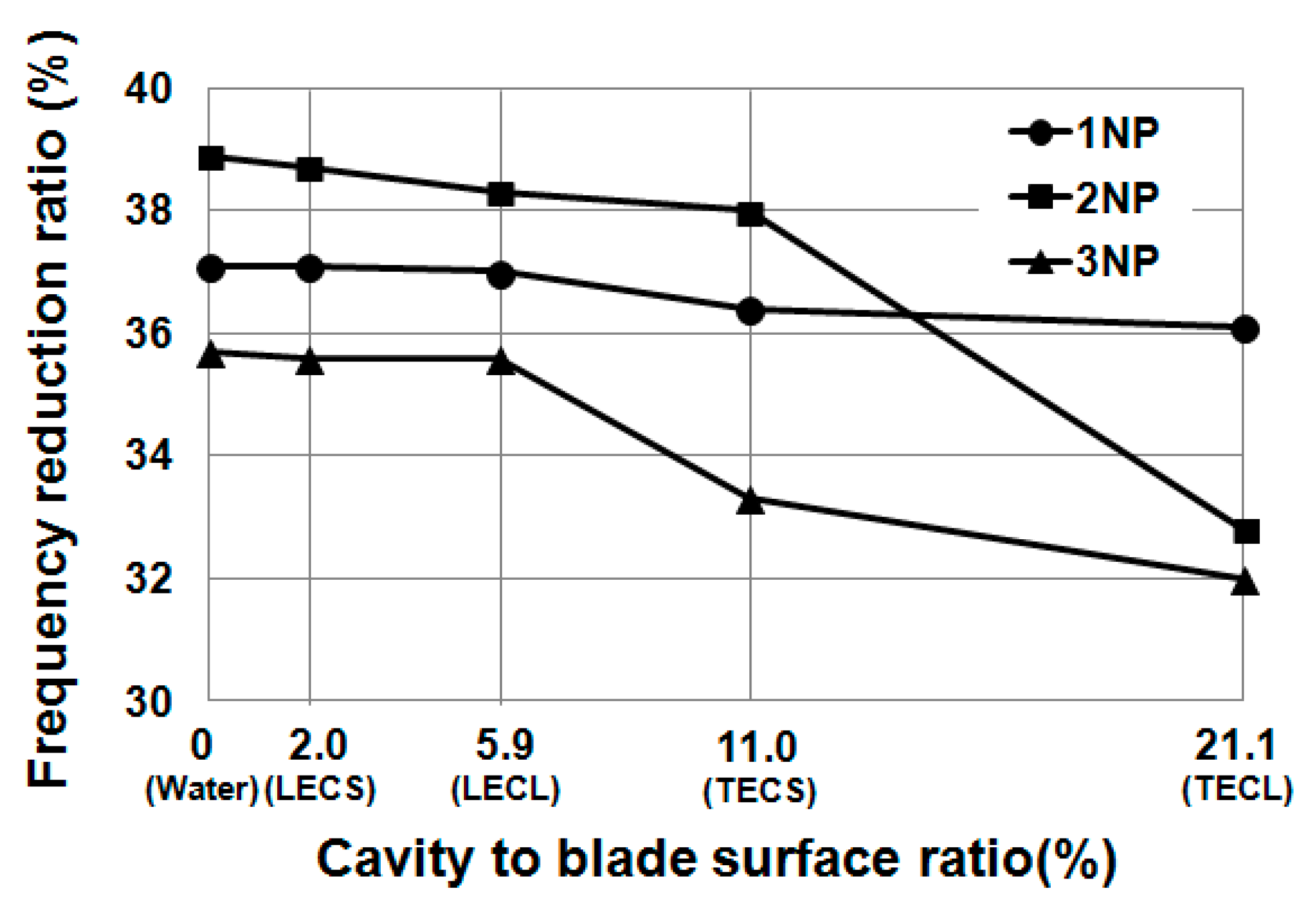
In order to quantitatively evaluate the added mass effects on the structures, the FRR of each mode either submerged in pure water (δw) or with various cavities (δcavity) has been calculated based on Equation (10). The deviation of FRRs of a specified mode due to the presence of different types of cavitation has been calculated with
δwδcavity = (fcavityfw)/fvacuum
where the frequency fcavity can correspond to any of the cavitation types fLECS, fLECL, fTECS and fTECL.
As the added mass effect of air on the modal behavior of structures has been experimentally and numerically proved to be negligible in similar studies [5,6,7,8,9,10], the numerical simulation to obtain the reference values will be performed in-vacuum conditions instead of air.
The procedure will consist of solving first the air condition, then the same case with water and finally with both water and attached pockets of vapor. This will be done first for a single blade to quantify the level of significance on the structure response. Then, the entire Francis runner will be simulated with air, water and water with cavitation. To conclude, the whole set of results will be compared among all the cases.

4. Modal Analysis of a Single Blade

4.1. Results for the Single-Phase Fluid

The dynamic response of a single blade both in air and submerged in a cylindrical water domain, as shown in Figure 5, is analyzed in order to evaluate the added water mass effects. Since the blades are welded to the crown and to the band to build the runner, all the degrees of freedom (DOFs) on the two tip sections of the single blade have been constrained.
Modal analysis of the first three modes of vibration shows that the largest blade deformations took place at the trailing edge. For the first mode, a single nodal point (NP) is found next to the mid span with no displacement relative to the static condition. For the second and third modes, two and three NPs are found, respectively. As a result, the number of NPs is used to identify the modes. In Figure 6, the blade deformation has been normalized to the maximum value for each mode where positive versus negative values indicate opposite directions of deformation. The calculated natural frequencies and the FRRs in air and water for the corresponding modes are indicated in Table 4.
It must be noted that the mode shapes in water present similar patterns to the ones obtained in air. Therefore, the results show that the same order of modes is found in water as in air. Nevertheless, the natural frequency of any specified mode in water is dramatically reduced due to the added water mass effect. In particular, the FRRs of the first three modes are found in the narrow range from 35% to 39%. These are the effects under expectation, given the fact that the deformed zones on the mode shape will vibrate simultaneously and accelerate the surrounding water. This will cause the so-called “added mass” of water on the structure and reduce the natural frequency.

4.2. Results for the Two-Phase Fluid

The natural frequencies and the FRRs of the first three modes of vibration, when considering the four different types of cavitation in the modal analysis, are listed in Table 5. They have been obtained by keeping the same boundary conditions as the case of a single-phase fluid. It must be noted that the presence of various types of cavities has no significant influence on the corresponding normalized blade mode shapes.
Figure 7 compares the natural frequencies of the single blade with pure water and with the different sizes and types of cavities. It is observed that, due to the presence of a vapor cavity, the natural frequency of each mode tends to be higher than the one in water without cavitation.
To compare the slight changes of frequencies observed for many cases with more precision, the deviations of FRRs calculated by Equation (16) are plotted for each mode in Figure 8. It is obvious that the deviations of FRRs observed in all the modes are almost negligible for any size of LEC. The increases of frequency are significant only for the large TEC in the case of the 2NP and 3NP modes, with a higher effect in 2NP. Meanwhile, for the small TEC, the 3NP mode is the most affected. The observed effects can be explained firstly by the size of the cavity and secondly by its location relative to the largest blade deformations for each mode shape.
To quantify the effect of cavity size, the CSR defined by Equation (15) has been correlated to the FRRs in Figure 9 for the three modes. It can be clearly observed that the added mass effect decreases when the ratio increases. Obviously, TEC has a larger influence on the natural frequencies than LEC. However, between the small and large sizes of TEC there is a sharp decrease of the FRR for the 2NP mode compared with the behavior of the other two modes. The FRR of 2NP is the highest for the first four cases shown in Figure 9. However, with the presence of TECL its value drops down and lies between the FRRs of 1NP and 3NP. This behavior might be due to the effect of the cavity location relative to the maximum blade deformations.
In Figure 10, the different cavity locations and sizes have been plotted on the mode shape graphs for the three modes. From this information it can be confirmed that there is a significant effect when the cavities are located in areas with larger blade deformations. Obviously, LEC is located in a region with almost no blade displacement for any mode. Contrarily, TEC covers partially or fully the large deformation zone on the blade for each mode shape. As a result, the added mass effects for LEC are almost the same as the case without cavitation, but for TEC the added mass effects are clearly reduced. For the 3NP mode, the deformation of the blade below the cavity is larger than for the 1NP and 2NP modes. As a result, the blade vibration accelerates more vapor and less water than for the other modes and, therefore, the added water mass effects on the blade for 3NP are lower. For the 2NP mode, the TECS covers the trailing edge up to the nodal point (see blue zone in Figure 10). However, when the cavity size is increased (as with the TECL), the nodal point is overcome and the cavity spans to the opposite deformation region (see the red zone in Figure 10) with a similar situation as the 3NP mode. As a result, the FRR of 2NP approaches that obtained for 3NP.

5. Modal Analysis of the Entire Turbine Runner

The investigation of the modal behavior of the entire Francis runner is necessary because the influence of attached cavitation on the structural response of the single blade has previously been proven. Based on such results, only the largest cavity dimensions for both LEC and TEC have been considered. For the numerical simulation, the same systematic method has been used as before.

5.1. Results for the Single-Phase Fluid

The Francis runners are typically fixed to the main turbine shaft with bolts. To calculate the structural response of the runner, all the DOFs on the contact surface between the runner and the shaft have been fixed to reproduce the constrained boundary condition properly. A large cylindrical tank, as shown on the right of Figure 11, has been considered to model the fluid domain surrounding the structure. The same material properties as the ones listed in Table 3 have been considered.
Table 6 presents the natural frequencies and corresponding FRRs for the first seven modes of vibration. The corresponding modes of vibration are shown in Figure 12, normalized by the corresponding maximum deformation value in each case. It can be seen that the vibration modes of the entire runner are very complex. The maximum deformation for all the modes appears on the blades. Because the deformation of the crown is relatively small, the mode shapes can be classified according to the deformation of the band and blades. The nodal diameter (ND) concept, a line that bisects the circle across the diameter, is used to characterize the mode shapes of the entire runner following the same criteria used by other authors [4,5]. The corresponding mode shape of the entire runner in air and in water keeps the same features.
Depending on the energy required to excite the vibration mode of the entire runner, the order of the mode shapes according to the frequency values indicated in Table 6 is 1ND, 0ND, 2ND, 3ND, 4ND, 5ND and 6ND. The surrounding water does not change the order of the runner modes. However, the presence of water results in a considerable frequency reduction for each mode.
From 1ND to 6ND, the runner has double modes with repeated natural frequencies. The features of each couple are the same, but the deformation distribution on the double modes has a spatial phase shift (Φ) given by
Φ = π/(2 × XND)
where XND is the ND number of a given mode.
Based on the observed mode shape movements represented in Figure 12, the 0ND runner mode corresponds to a torsion motion around the axis of rotation combined with an elevation motion in the axial direction. Moreover, all blades present the same in phase deformation and movement. For 1ND, the runner swings like a pendulum and the blades can be divided into two groups depending on the relative phase of their deformation. In both groups, the blades vibrate in phase inside their own groups, but in counter phase between the two groups. From 2ND to 6ND, high deformation also appears on the band, although a little lower than that of the blades. Like 1ND, the blades of the modes from 2ND to 6ND can also be divided into 2 × XND groups. The blades inside their own groups vibrate in phase, but in the adjacent groups they vibrate in counter phase.
From the differences between natural frequencies observed in Figure 13, it is confirmed that the added water mass effect depends on the deformation shapes of the modes. In particular, the FRR increases with XND, as shown in Figure 14, which is used to classify the mode shapes. So, 0ND has the lowest FRR, with a value of 10.2%, and 6ND has the maximum FRR with a value of 47.5%. This can be explained by the fact that the two lowest modes, 0ND and 1ND, accelerate less water than the modes with higher XND that have larger deformations in the normal directions to the blade and band surfaces.
To finish, the regression analysis plotted in Figure 14 demonstrates an accurate linear relationship between FRR and XND. Therefore, a simple law can be used to calculate the natural frequencies of the submerged runner in water for any mode.

5.2. Results for the Two-Phase Fluid

As shown in Figure 15, the large size for both types of cavitation in the single blade, LECL and TECL, have also been modeled on all the blades of the investigated Francis runner in separate cases. The thickness of the attached cavities is 0.225 m, the same as that of the single blade. The vapor volume fraction is also 1, and the same material properties of structure, fluid and vapor shown in Table 3 are used. The obtained natural frequencies and FRRs are indicated in Table 7. Then, the natural frequencies of the runner submerged in pure water and with cavitation are compared in Figure 16.
The presence of cavities does not change the order of the natural frequencies of the runner. However, the cavities have a small but clear influence on the value of the natural frequencies. For all modes shown in Figure 12, the natural frequencies of the submerged runner with cavitation are increased compared with the corresponding ones in water without cavitation. The influence of the TECL on the natural frequencies is larger than that of the LECL.
In order to evaluate the added mass effect of attached cavitation on each mode in detail, the differences of FRRs of each mode when cavities exist have been plotted in Figure 17. The results confirm that the added water mass effects are reduced with the presence of cavitation. The TECL induces a larger reduction than the LECL as occurred on the single blade. The most influenced modes are 1ND and 2ND, with more than 4% difference in both types of cavitation. It must be noted that for the entire runner, the global effect of LECL is significant for all modes with values above 1%, which was not the case with the single blade. As the ND number increases, it is also observed how the effects decrease.
Similar to the single blade, the added mass effects of cavitation attached to the blade are influenced by the runner mode shapes and the locations of the cavities. For all extracted modes, the blade trailing edges have a much larger deformation because they are thinner than the leading edges. Furthermore, the TECL covers a lager deformed zone on the blade than the LECL. As a result, TECL has a larger influence than LECL on the added water mass.
The results indicate that the most affected mode of vibration is 2ND for both types of cavitation. This might be explained by the fact that in this case the blade surfaces covered by LECL and TECL vibrate in their normal direction (as shown in Figure 18), which has a strong influence on the added mass effects. For other modes with higher XND, although they also have a normal deformation on blades, the total region in contact with the cavity surface is lower than for 2ND. Finally, 0ND and 1ND do not present such movement, due to their completely different movement.
Furthermore, the FRRs of all the runner modes in water with and without cavities have been plotted in Figure 19. The results indicate that the added mass effects with cavities attached to the blades are smaller than those with blade without cavities surrounded by only water. The FRRs of the runner with cavities also present a very precise linear relationship with XND in all cases. Nevertheless, the fitted line for the case without cavities has a smaller slope but larger intercept than the line estimated for the case with cavities.
In summary, the linear regressions permitting calculation of the FRRs of the runner when submerged in pure water, in water with the LECL or in water with the TECL, are indicated in Equations (18)–(20), respectively, as a function of the mode order.
δ w = 6.36 ( X N D + 1 ) + 4.94
δ L E C L = 6.78 ( X N D + 1 ) + 0.45
δ T E C L = 6.65 ( X N D + 1 ) 0.13

6. Conclusions

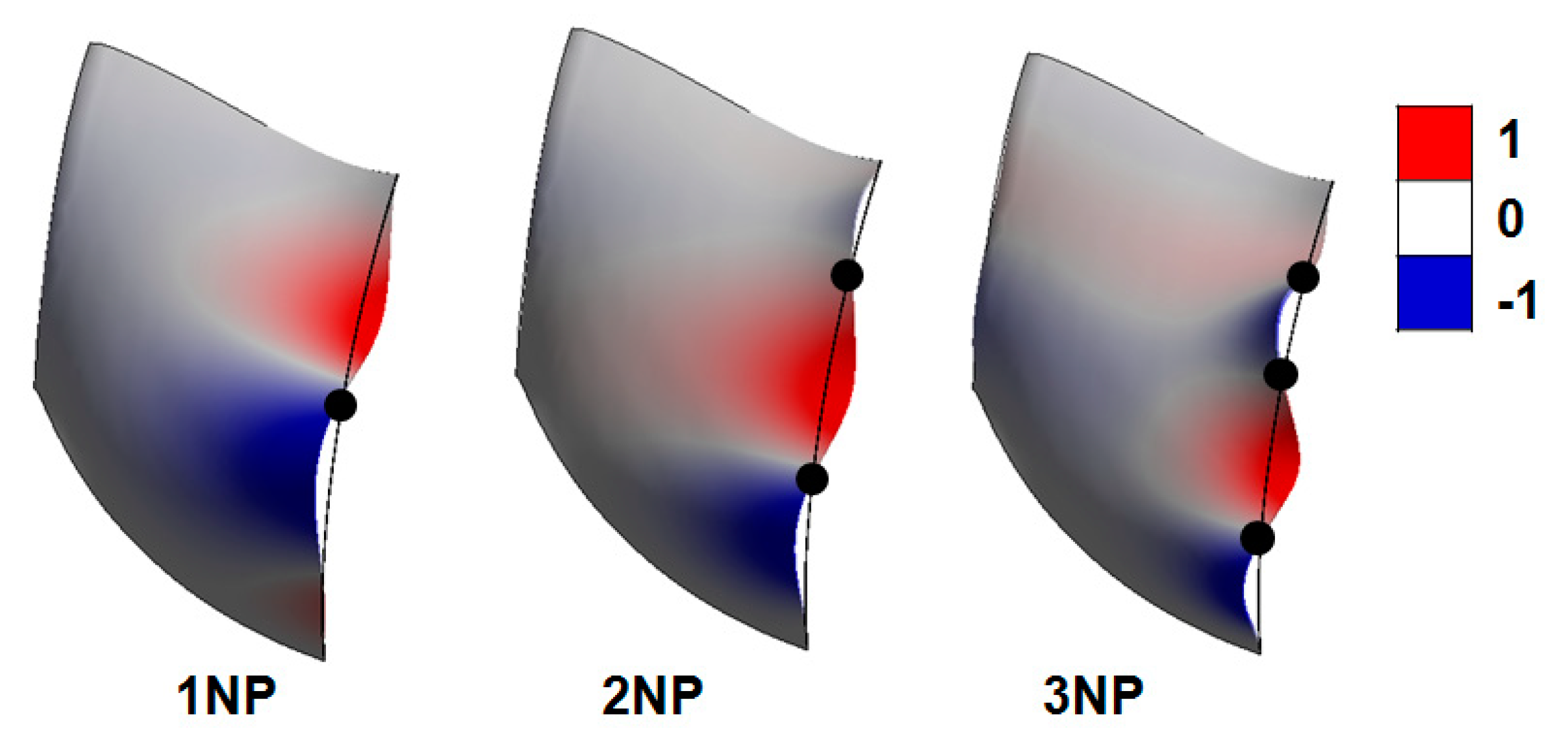
The added mass effects of attached blade cavitation on the structural behavior of a single blade and of a complete Francis runner have been investigated numerically. The acoustic–structural coupling method was applied to calculate the natural frequencies and mode shapes of the structure surrounded by a fluid. The study compared the results of a single-phase fluid, water, with those of a two-phase fluid, vapor and water, by reproducing the typical leading edge or trailing edge attached blade cavitation.
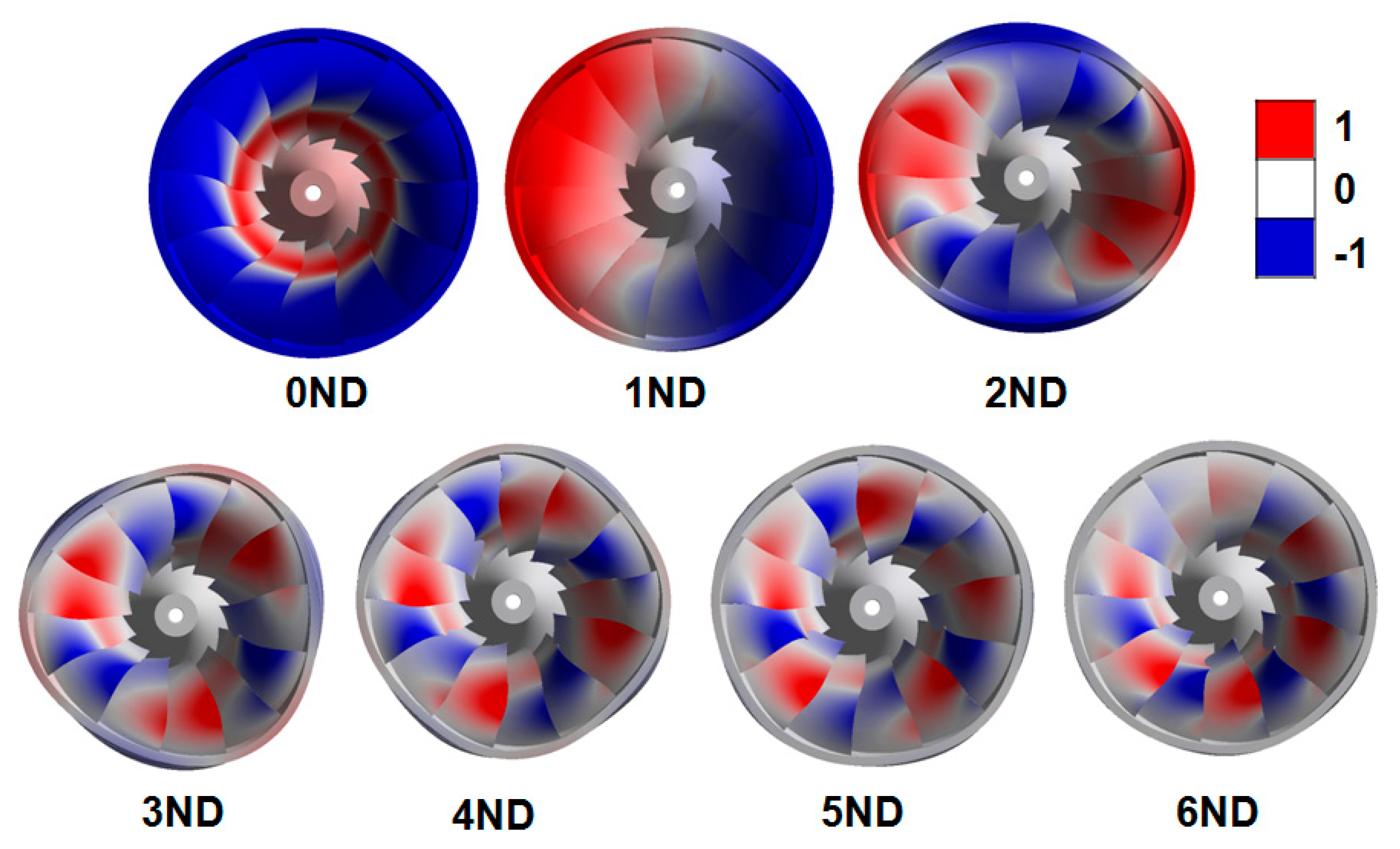
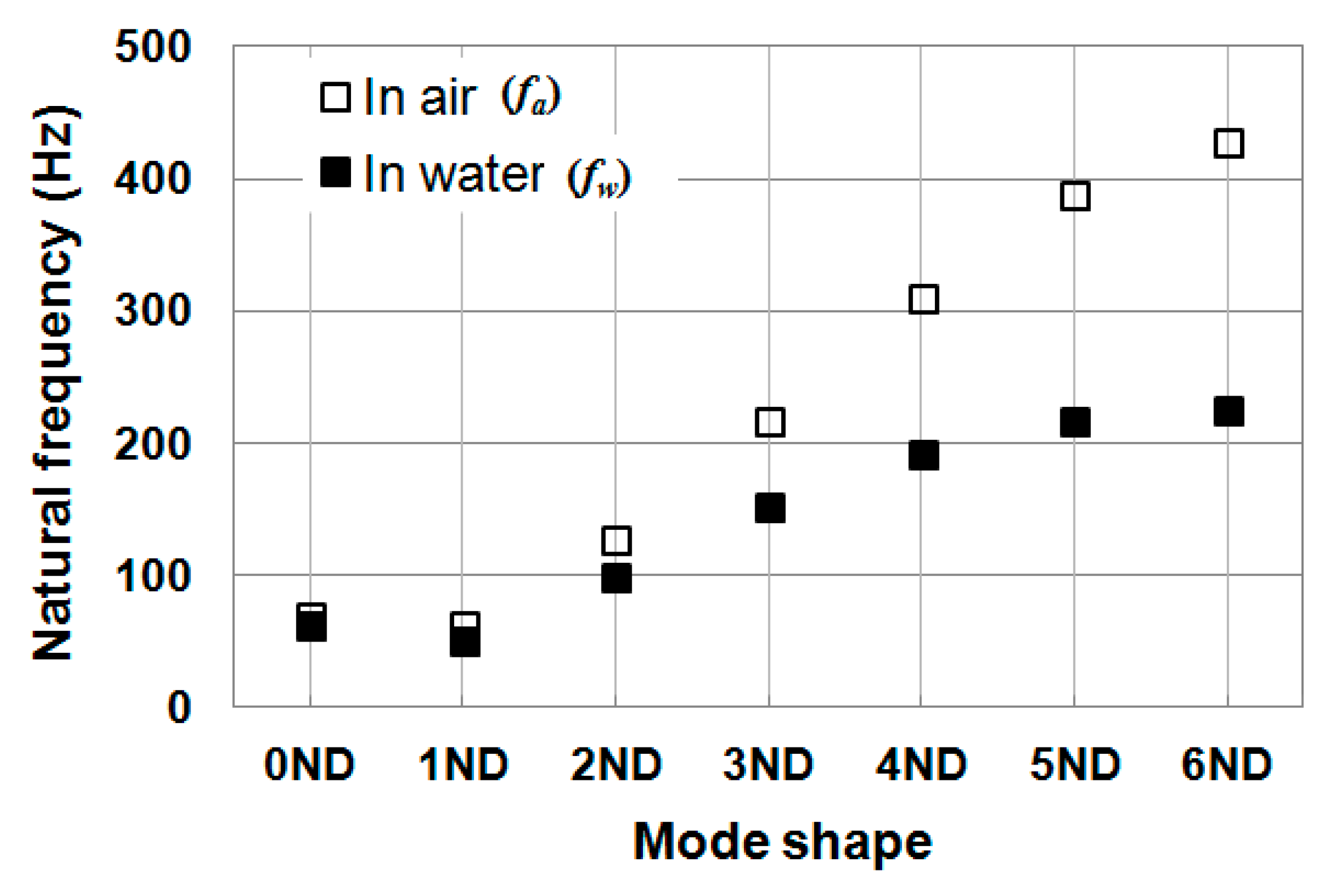
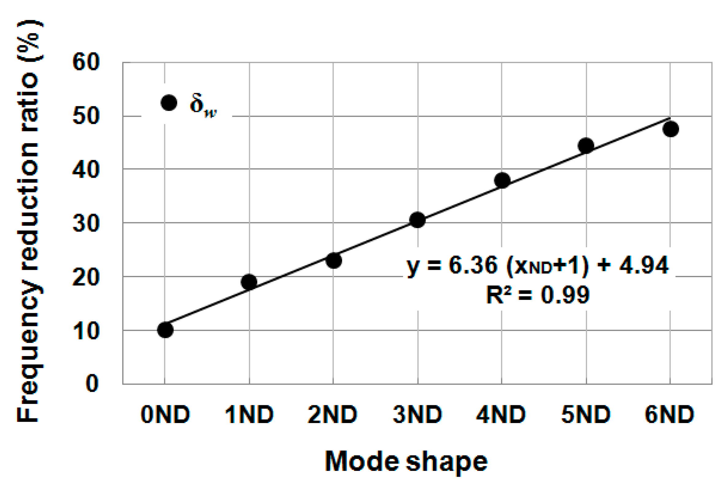
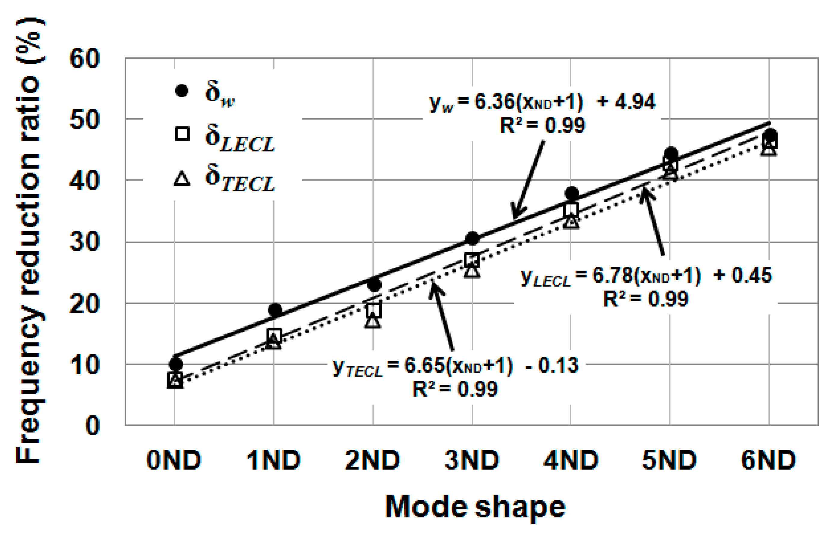
Surrounding water led to a significant reduction of natural frequencies. For the single blade, the first three natural frequencies were reduced by around 37%. For the whole runner, the first seven natural frequencies were reduced from around 10% to 48%, following a growing linear trend with the nodal diameter number. Therefore, added water mass effects depend on mode shape. The modes that present more deformation in the direction normal to the blade surface have larger added water mass effects because they accelerate more surrounding fluid.
In general, the presence of vapor cavities on the blades provoked an increase of natural frequencies due to a reduction of added mass for both the single blade and the whole runner.
For the single blade, only trailing edge cavitation presented more than 1% effect for the second and third modes. The largest influence was found for the second mode, at about 6% for the large cavity size. This behavior was determined by the effective normal deformation of the blade at the cavity location as well as the size of the cavity. For the same reason, the effects of leading edge cavitation were lower than 1% due to the low deformation of the blade and smaller size.
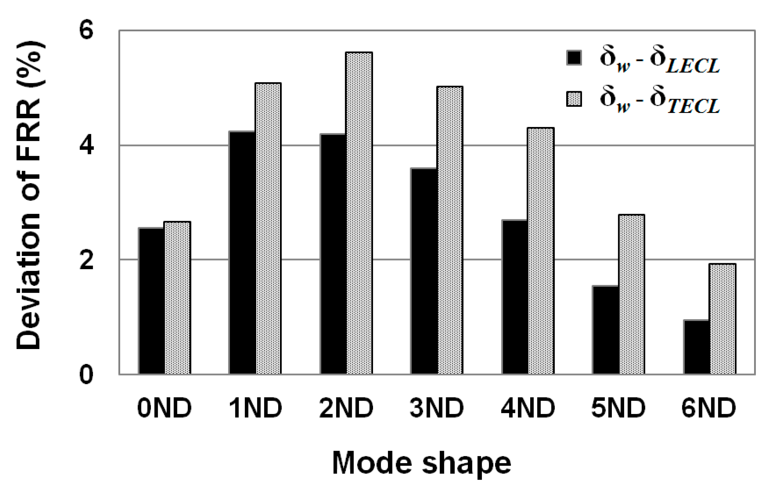
For the entire runner, both leading and trailing edge cavities induced effects higher than 1% in all modes because the mode shapes of the blades differed in relation to the single blade case. As a result, the maximum effects were found between 4% and 6% for modes 1ND and 2ND with both types of cavitation. Starting from 2ND, the effects decreased with nodal number. Again, trailing edge cavitation always had a larger effect than leading edge cavitation for any given mode.
In summary, added mass effects with cavitation attached to blades was determined by the coincidence between the mode shape of the structure and the location and size of the cavities. However, the main features of the mode shape were similar in all the cases considered. In reality, a Francis runner is mounted inside a spiral case in a hydropower plant, and the added mass effects of attached cavitation on a submerged runner with nearby boundaries should be further investigated.

Author Contributions

Conceptualization and methodology, X.H. and X.E.; investigation X.H.; writing—original draft preparation, X.H.; writing—review and editing, X.H. and X.E.

Funding

This research received no external funding.

Conflicts of Interest

The authors declare no conflict of interest.

Abbreviations

AFSCMAcoustic fluid–structural coupling method
DOFDegree of freedom
FEMFinite element method
FRRFrequency reduction ratio
LECLeading edge cavitation
LECLLarge leading edge cavitation
LECSSmall leading edge cavitation
NDNodal diameter
NPNodal point
TECTrailing edge cavitation
TECLLarge leading edge cavitation
TECSSmall trailing edge cavitation

References

  1. Escaler, X.; Egusquiza, E.; Farhat, M.; Avellan, F. Detection of Cavitation in Hydraulic Turbines. Mech. Syst. Signal Process 2006, 20, 983–1007. [Google Scholar] [CrossRef]
  2. International Standard IEC 60193:2019 Hydraulic Turbines, Storage Pumps and Pump-Turbines—Model Acceptance Tests. Available online: https://webstore.iec.ch/publication/60951 (accessed on 13 May 2019).
  3. Avellan, F. In Introduction to cavitation in hydraulic machinery. In Proceedings of the 6th International Conference on Hydraulic Machinery and Hydrodynamics, Timisoara, Romania, 21–22 October 2004. [Google Scholar]
  4. Egusquiza, E.; Valero, C.; Huang, X.; Jou, E.; Guardo, A.; Rodriguez, C.G. Failure investigation of a large pump-turbine runner. Eng. Fail. Anal. 2012, 23, 27–34. [Google Scholar] [CrossRef] [Green Version]
  5. Trivedi, C.; Cervantes, M. Fluid-structure interactions in Francis turbines: A perspective review. Renew. Sustain. Energy Rev. 2017, 68, 87–101. [Google Scholar] [CrossRef]
  6. Huang, X.; Chamberland-Lauzon, J.; Oram, C.; Klopfer, A.; Ruchonnet, N. Fatigue analyses of the prototype Francis runners based on site measurements and simulations. IOP Conf. Ser. Earth Environ. Sci. 2014, 22, 012014. [Google Scholar] [CrossRef] [Green Version]
  7. Valentin, D.; Presas, A.; Bossio, M.; Egusquiza, M.; Egusquiza, E.; Valero, C. Feasibility of Detecting Natural Frequencies of Hydraulic Turbines While in Operation, Using Strain Gauges. Sensors 2018, 18, 174. [Google Scholar] [CrossRef] [PubMed]
  8. Tanaka, H. In Vibration and dynamic stress of runners of very high head reversible pump-turbines. In Proceedings of the 15th IAHR Symposium on Hydraulic Machinery and Systems, Belgrade, Yugoslavia, 11–14 September 1990. [Google Scholar]
  9. Huang, X.; Oram, C.; Sick, M. Static and dynamic stress analyses of the prototype high head Francis runner based on site measurement. IOP Conf. Ser. Earth Environ. Sci. 2014, 22, 032052. [Google Scholar] [CrossRef] [Green Version]
  10. Rodriguez, C.G.; Egusquiza, E.; Escaler, X.; Liang, Q.W. Experimental investigation of added mass effects on a Francis turbine runner in still water. J. Fluid Struct. 2006, 22, 699–712. [Google Scholar] [CrossRef]
  11. Liang, Q.W.; Rodriguez, C.G.; Egusquiza, E.; Escaler, X. Numerical simulation of fluid added mass effect on a Francis turbine runner. Comput. Fluids 2007, 36, 1106–1118. [Google Scholar] [CrossRef]
  12. Escaler, X.; Hütter, J.K.; Egusquiza, E.; Farhat, M.; Avellan, F. Modal behavior of a reduced scale pump-turbine impeller. Part 1: Experiments. IOP Conf. Ser. Earth Environ. Sci. 2010, 12, 012116. [Google Scholar] [CrossRef]
  13. Valero, C.; Huang, X.; Egusquiza, E.; Farhat, M.; Avellan, F. Modal behavior of a reduced scale pump-turbine impeller. Part 2: Numerical simulation. IOP Conf. Ser. Earth Environ. Sci. 2010, 12, 012117. [Google Scholar] [CrossRef]
  14. Dehkharqani, A.; Aidanpää, J.; Engström, F.; Cervantes, M. A Review of Available Methods for the Assessment of Fluid Added Mass, Damping, and Stiffness with an Emphasis on Hydraulic Turbines. ASME Appl. Mech. Rev. 2019, 70, 050801. [Google Scholar] [CrossRef]
  15. Huang, X.; Egusquiza, E.; Valero, C.; Presas, A. Dynamic behaviour of pump-turbine runner: From disk to prototype runner. IOP Conf. Ser. Earth Environ. Sci. 2013, 52, 022036. [Google Scholar] [CrossRef]
  16. Huang, X.; Valero, C.; Egusquiza, E. In The effect on boundary condition on the structural response of a pump-turbine. In Proceedings of the 3rd IAHR International Meeting of the Workgroup on Cavitation and Dynamic Problems in Hydraulic Machinery and Systems, Brno, Czech Republic, 14–16 October 2009. [Google Scholar]
  17. Huang, X. Contribution to the Dynamic Response of Hydraulic Turbomachinery Components. Ph.D. Thesis, Universitat Politècnica de Catalunya, Catalunya, Spain, 2011. [Google Scholar]
  18. Presas, A.; Valero, C.; Huang, X.; Egusquiza, E.; Farhat, M.; Avellan, F. Analysis of the dynamic response of pump-turbine runners-Part I: Experiment. IOP Conf. Ser. Earth Environ. Sci. 2012, 15, 052015. [Google Scholar] [CrossRef]
  19. Liu, X.; Luo, Y.; Presas, A.; Wang, Z.; Zhou, L. Cavitation Effects on the Structural Resonance of Hydraulic Turbines: Failure Analysis in a Real Francis Turbine Runner. Energies 2018, 11, 2320. [Google Scholar] [CrossRef]
  20. De La Torre, O.; Escaler, X.; Egusquiza, E.; Farhat, M. Experimental investigation of added mass effects on a hydrofoil under cavitation conditions. J. Fluid Struct. 2013, 39, 173–187. [Google Scholar] [CrossRef] [Green Version]
  21. Liu, X.; Zhou, L.; Wang, Z.; Escaler, X.; Luo, Y.; De La Torre, O. Numerical simulation of added mass effects on a hydrofoil in cavitating flow using acoustic FSI. J. Fluid Eng. Trans. ASME 2017, 139, 8. [Google Scholar] [CrossRef]
  22. Celebioglu, K.; Altintas, B.; Aradag, S.; Tascioglu, Y. Numerical research of cavitation on Francis turbine runners. Int. J. Hydrogen Energy 2017, 42, 17771–17781. [Google Scholar] [CrossRef]
  23. Müller, A.; Favrel, A.; Landry, C.; Avellan, F. Fluid–structure interaction mechanisms leading to dangerous power swings in Francis turbines at full load. J. Fluid Struct. 2017, 69, 56–71. [Google Scholar] [CrossRef]
  24. Escaler, X.; Vilberg, I.K.; Ekanger, J.V.; Francke, H.H.; Kjeldsen, M. Assessment of Remote Cavitation Detection Methods with Flow Visualization in a Full Scale Francis Turbine. In Proceedings of the 10th International Symposium on Cavitation (CAV2018), Baltimore, MD, USA, 14–16 May 2018; Katz, J., Ed.; ASME: New York, NY, USA, 2018. [Google Scholar]
  25. Lamb, H. Hydrodynamics, 6th ed.; The Syndics of the Cambridge at the University Press: New York, NY, USA, 1952; pp. 76–77. [Google Scholar]
  26. Milne-Thomson, L.M. Theoretical Hydrodynamics, 5th ed.; Macmillan Education LTD: London, UK, 1968; pp. 246–249. [Google Scholar]
  27. Brennen, C.E.; Naval Civil Engineering Laboratory, Port Hueneme, CA, USA. A review of added mass and fluid inertial forces. Personal communication, 1982. [Google Scholar]
  28. ANSYS, Inc. 8.4. Acoustic Fluid-Structural Interaction (FS). In ANSYS Mechanical APDL Theory Reference; Kohnke, P., Ed.; ANSYS, Inc.: Canonsburg, PA, USA, 2013; Release 15.0; pp. 276–280. [Google Scholar]
Figure 1. Geometry and the main dimensions of the investigated Francis runner.
Fluids 04 00107 g001
Figure 2. (a) Sizes and locations of the simulated leading edge cavitation on the single blade; (b) sizes and locations of the simulated trailing edge cavitation on the single blade.
Fluids 04 00107 g002
Figure 3. (a) Sensitivity analysis of the mesh density for the single blade; (b) sensitivity analysis of the mesh density for the entire turbine runner.
Fluids 04 00107 g003
Figure 4. (a) Mesh of the single blade and the surrounding water; (b) mesh of the entire runner and the surrounding water.
Fluids 04 00107 g004
Figure 5. (a) Geometry and boundary conditions of a single blade in air; (b) geometry and dimensions of the surrounding cylindrical water domain.
Fluids 04 00107 g005
Figure 6. Shapes of the first three modes of vibration of the single blade.
Fluids 04 00107 g006
Figure 7. Natural frequencies of the single blade with pure water and with different cavities.
Fluids 04 00107 g007
Figure 8. Comparison of the deviation of FRRs for the single blade.
Fluids 04 00107 g008
Figure 9. Comparison of the FRRs of the single blade with pure water and with different cavities.
Fluids 04 00107 g009
Figure 10. Cavity locations marked on the mode shape graphs of the single blade.
Fluids 04 00107 g010
Figure 11. (a) Geometry and boundary conditions of the runner in air; (b) geometry and dimensions of the surrounding cylindrical water domain.
Fluids 04 00107 g011
Figure 12. Bottom view of the Francis runner mode shapes in air with normalized deformations.
Fluids 04 00107 g012
Figure 13. Natural frequencies of the runner in air and in water.
Fluids 04 00107 g013
Figure 14. Linear fit between the FRR and the ordered modes of vibration.
Fluids 04 00107 g014
Figure 15. (a) Size and location of the leading edge attached cavitation on the blades of the runner; (b) size and location of the trailing edge attached cavitation on the blades of the runner.
Fluids 04 00107 g015
Figure 16. Natural frequencies of the runner with pure water and with different cavities.
Fluids 04 00107 g016
Figure 17. Comparison of the deviation of FRRs for the runner.
Fluids 04 00107 g017
Figure 18. (a) Lateral view of the 2ND deformation in the area with leading edge cavitation; (b) lateral view of the 2ND deformation in the area with trailing edge cavitation.
Fluids 04 00107 g018
Figure 19. Linear fits between the FRRs and the ordered modes of vibration.
Fluids 04 00107 g019
Table 1. Cavity to blade surface ratio of small leading edge cavitation (CSRLECS), of large leading edge cavitation (CSRLECL), of small trailing edge cavitation (CSRTECS) and of large trailing edge cavitation (CSRTECL).
CSRLECSCSRLECLCSRTECSCSRTECL
2.05.911.021.1
Table 2. Number of elements of the various meshes for the structure and fluid domains.
Blade StructureBlade FluidRunner StructureRunner Fluid
3.1 × 1032.1 × 1041.1 × 1051.2 × 106
Table 3. Density (ρs), Young’s modulus (E) and Poisson’s ratio (ν) of the structure; density (ρw) and sonic speed (cw) of the water; and density (ρv) and sonic speed (cv) of the vapor.
ρs [kg/m3]E [GPa]ν [-]ρw [kg/m3]cw [m/s]ρv [kg/m3]cv [m/s]
77002060.3100014820.0172423
Table 4. Natural frequencies in air (fa) and water (fw), and frequency reduction ratios (δw) of the single blade modes with 1, 2 and 3 nodal points (NP).
Modefa [Hz]fw [Hz]δw [%]
1NP513.2323.037.1
2NP589.9360.438.9
3NP826.1531.235.7
Table 5. Natural frequencies (f) and frequency reduction ratios (δ) of the single blade with cavitation.
ModefLECS [Hz]fLECL [Hz]fTECS [Hz]fTECL [Hz]δLECS [%]δLECL [%]δTECS [%]δTECL [%]
1NP323.0323.1326.2327.537.137.036.436.1
2NP361.4363.5365.2394.938.738.338.032.8
3NP531.6531.9548.9557.235.635.633.332.0
Table 6. Natural frequencies in air (fa) and in water (fw), and frequency reduction ratios (δw) of the runner modes from 0 to 6 nodal diameters (ND).
Modefa [Hz]fw [Hz]δw [%]
0ND68.461.410.2
1ND61.750.018.9
2ND126.697.523.0
3ND216.8150.330.7
4ND308.9191.538.0
5ND388.1215.644.4
6ND427.5224.247.5
Table 7. Natural frequencies of the runner with cavitation (f) and frequency reduction ratios (δ) of the modes from 0 to 6 nodal diameters (ND).
ModefLECL [Hz]fTECL [Hz]δLECL [%]δTECL [%]
0ND63.263.37.67.5
1ND52.653.114.713.9
2ND102.8104.618.817.4
3ND158.1161.227.125.6
4ND199.9204.835.333.7
5ND221.6226.442.941.7
6ND228.3232.446.645.6

