Closure Relations for Fluxes of Flame Surface Density and Scalar Dissipation Rate in Turbulent Premixed Flames

Abstract

In this study, closure relations for total and turbulent convection fluxes of flame surface density and scalar dissipation rate were developed (i) by placing the focus of consideration on the flow velocity conditioned to the instantaneous flame within the mean flame brush and (ii) by considering the limiting behavior of this velocity at the leading and trailing edges of the flame brush. The model was tested against direct numerical simulation (DNS) data obtained from three statistically stationary, one-dimensional, planar, premixed turbulent flames associated with the flamelet regime of turbulent burning. While turbulent fluxes of flame surface density and scalar dissipation rate, obtained in the DNSs, showed the countergradient behavior, the model predicted the total fluxes reasonably well without using any tuning parameter. The model predictions were also compared with results computed using an alternative closure relation for the flame-conditioned velocity.

1. Introduction

Among various approaches to modeling premixed turbulent combustion, concepts that deal with a transport equation for the mean flame surface density (FSD) 〈Σ〉 = 〈|∇c|〉 [1,2] or the Favre-averaged scalar dissipation rate (SDR) 〈χ〉^~ = 〈ρD∇c∙∇c〉/〈ρ〉 [3] have become particularly popular over the past decade [4,5,6]. Here, c is the combustion progress variable, which characterizes the state of a reacting mixture in a flame, and is equal to zero and unity in unburned reactants and equilibrium combustion products, respectively, ρ is the mixture density, D is the molecular diffusivity of c, and 〈q〉 and 〈q〉^~ = 〈ρq〉/〈ρ〉 designate the Reynolds and Favre (i.e., mass-weighted), respectively, mean values of an arbitrary quantity q. As reviewed elsewhere [4,5,6], both transport equations involve a number of terms that should be modeled, but the present communication is solely restricted to total transport terms 〈uΣ〉 = 〈u〉〈Σ〉 + 〈u′Σ′〉 and 〈ρuχ〉 = 〈ρ〉〈u〉^~〈χ〉^~ + 〈ρu″χ″〉, turbulent contributions to which (i.e., 〈u′Σ′〉 and 〈ρu″χ″〉) require closure relations. Here, u is the flow velocity vector, and q′ = q − 〈q〉 and q″ = q − 〈q〉^~ are fluctuations of q with respect to its Reynolds and Favre-averaged values, respectively.

As reviewed elsewhere [4,5,6], in applications, the turbulent transport terms are commonly modeled invoking a paradigm of gradient diffusion, for example, 〈u′Σ′〉 = −D_t∇〈Σ〉 and 〈ρu″χ″〉 = −〈ρ〉D_t∇〈χ〉^~, where D_t > 0 is turbulent diffusivity. However, at least for the turbulent flux 〈ρu″c″〉 of the combustion progress variable c, such a paradigm is challenged by countergradient turbulent transport [7,8], that is, 〈ρu″c″〉∙∇〈c〉^~ > 0, which is well documented in various flames, as reviewed elsewhere [9,10,11]. For the FSD or SDR concept, an issue of eventually countergradient flux of 〈u′Σ′〉 or 〈ρu″χ″〉 is of particular importance, because the corner-stone assumption of the two concepts (i.e., a linear relation between the mean mass rate 〈W〉 of creation of c and ρ_u〈Σ〉 [1,2] or 〈ρ〉〈χ〉^~ [3]) is best justified under conditions of the flamelet combustion regime [12], which are commonly associated with the countergradient transport [9,10,11]. Accordingly, the goal of the present work is to suggest and validate simple closure relations capable of predicting the total convection fluxes 〈uΣ〉 = 〈u〉〈Σ〉 + 〈u′Σ′〉 and 〈ρuχ〉 = 〈ρ〉〈u〉^~〈χ〉^~ + 〈ρu″χ″〉 and, in particular, the countergradient turbulent fluxes 〈u′Σ′〉 and 〈ρu″χ″〉 in the flamelet combustion regime.

In the next section, the developed model is presented and the direct numerical simulation (DNS) data used to access it are summarized. In the third section, results of the model validation using the DNS data are discussed and the model is compared with alternative approaches. Conclusions are drawn in the fourth section.

2. Method of Research

2.1. Model

Using velocities

〈u〉_f,Σ = 〈uΣ〉/〈Σ〉

(1)

and

〈u〉_f,χ = 〈ρuχ〉/〈ρχ〉

(2)

conditioned to flamelets, modeling of the total fluxes 〈uΣ〉 = 〈u〉_f,Σ〈Σ〉 and 〈ρuχ〉 = 〈u〉_f,χ〈ρ〉〈χ〉^~ in the transport equations for 〈Σ〉 and 〈χ〉^~, respectively, is reduced to modeling the conditioned velocities, whereas closure relations for the turbulent fluxes 〈u′Σ′〉 and 〈ρu″χ″〉 are not required.

In order to model the conditioned velocities, let us start with a discussion of a constant-density flow. In such a case, the following simple closure relation,

〈u〉_f = (1 − 〈c〉)〈u〉_b + 〈c〉〈u〉_u,

(3)

was proposed [13] and validated in a recent DNS study [14] of self-propagation of an infinitely thin interface in a constant-density turbulent flow. Here, 〈u〉_f is velocity conditioned to the interface, subscripts u and b designate quantities conditioned to reactants and products, respectively, which are separated by the interface. Note that the conditioned velocities 〈u〉_u and 〈u〉_b vary along the normal to the mean reaction wave. For instance, in the statistically 1D, planar, and stationary case, 〈u〉_u = 〈u〉_u(x) and 〈u〉_b = 〈u〉_b(x) if the x-axis is normal to the mean wave, with averaging being performed over transverse planes.

Equation (3) is based on the following simple physical reasoning. For an infinitely thin interface, its arrival to the trailing edge of a mean reaction-wave brush is always accompanied by the arrival of reactants to the same trailing point. Therefore, 〈u〉_f→〈u〉_u at 〈c〉→1. Due to similar arguments, 〈u〉_f→〈u〉_b at 〈c〉→0. Thus, Equation (3) is nothing more than a linear interpolation between two limiting relations.

Let us assume that the same interpolation holds both for 〈u〉_f,Σ and 〈u〉_f,χ, that is, 〈u〉_f,Σ = 〈u〉_f,χ = 〈u〉_f, in the case of a constant-density “flamelet” of a finite thickness. Such an assumption is based on a small thickness of a flamelet when compared to a mean flame brush thickness in a typical case.

If we allow for combustion-induced thermal expansion, effects due to the finite flamelet thickness appear to be of more importance due to significant velocity variations within thin flamelets. In particular, 〈u〉_f,b∙n < 〈u〉_f∙n < 〈u〉_f,u∙n, because local flow acceleration within a flamelet occurs in the direction opposite to the direction of a unit vector n = −∇c/|∇c| that is locally normal to the flamelet (i.e., (〈u〉_f,b − 〈u〉_f,u)∙n < 0). Here, 〈u〉_f,u and 〈u〉_f,b are evaluated on the reactant and product sides of the flamelet along the local normal to it. Because the peak value of Σ(c) or χ(c) is shifted to the product side of a typical laminar premixed flame, the simplest way to allow for the discussed difference between the conditioned velocities 〈u〉_f,u, 〈u〉_f, and 〈u〉_f,b appears to consist in (i) neglecting the difference in 〈u〉_f,Σ or 〈u〉_f,χ and 〈u〉_f,b→〈u〉_b at 〈c〉→0, but (ii) assuming that both |〈u〉_f,b − 〈u〉_f,Σ| ≪ |〈u〉_f,b − 〈u〉_f,u| and |〈u〉_f,b − 〈u〉_f,χ| ≪ |〈u〉_f,b − 〈u〉_f,u| at 〈c〉→1. For example,

(〈u〉_f,b − 〈u〉_f,Σ)=σ⁻¹(〈u〉_f,b − 〈u〉_f,u) or (〈u〉_f,b − 〈u〉_f,χ) = σ⁻¹(〈u〉_f,b − 〈u〉_f,u)

in order to avoid invoking tuning parameters. Here, σ = ρ_u/ρ_b is the density ratio. Consequently,

〈u〉_f,Σ→σ⁻¹〈u〉_f,u + (1 − σ⁻¹)〈u〉_f,b and 〈u〉_f,χ→σ⁻¹〈u〉_f,u + (1 − σ⁻¹)〈u〉_f,b at 〈c〉→1.

If we further assume that 〈u〉_f,b = 〈u〉_b at 〈c〉→1, then,

〈u〉_f,Σ→σ⁻¹〈u〉_u + (1 − σ⁻¹)〈u〉_b and 〈u〉_f,χ→σ⁻¹〈u〉_u + (1 − σ⁻¹)〈u〉_b at 〈c〉→1.

Note that 〈u〉_f,u→〈u〉_u at 〈c〉→1, because the unburned gas can arrive at the trailing edge of the mean flame brush only together with a flamelet. Finally, since 〈u〉_b = 〈u〉 = 〈u〉^~ at 〈c〉 = 1, we arrive at

〈u〉_f,Σ→σ⁻¹〈u〉_u + (1 − σ⁻¹)〈u〉^~ and 〈u〉_f,χ→σ⁻¹〈u〉_u + (1 − σ⁻¹)〈u〉^~ at 〈c〉→1

or

(〈u〉_f,Σ − 〈u〉^~)→σ⁻¹(〈u〉_u − 〈u〉^~) and (〈u〉_f,χ − 〈u〉^~)→σ⁻¹(〈u〉_u − 〈u〉^~) at 〈c〉→1.

Thus, in the case of σ > 1, we have the following two approximate limiting relations: 〈u〉_f,Σ→〈u〉_b or 〈u〉_f,χ→〈u〉_b at 〈c〉→0 and (〈u〉_f,Σ − 〈u〉^~)→σ⁻¹(〈u〉_u − 〈u〉^~) or (〈u〉_f,χ − 〈u〉^~)→σ⁻¹(〈u〉_u − 〈u〉^~) at 〈c〉→1. Then, linear interpolation results in

〈u〉_f,Σ − 〈u〉^~ = 〈c〉σ⁻¹(〈u〉_u − 〈u〉^~) + (1 − 〈c〉)(〈u〉_b − 〈u〉^~)

(4)

and

〈u〉_f,χ − 〈u〉^~ = 〈c〉σ⁻¹(〈u〉_u − 〈u〉^~) + (1 − 〈c〉)(〈u〉_b − 〈u〉^~).

(5)

In the case of σ = 1 (constant density), Equations (4) and (5) reduce to Equation (3) and yield correct values of 〈u〉_f,Σ and 〈u〉_f,χ at least at the boundaries 〈c〉→0 and 〈c〉→1 of the mean “flame” brush.

It is worth noting that Equations (4) and (5) extend Equation (3) by allowing for effects due to density variations and finite flamelet thickness. Since such an extension was performed by invoking a few simple assumptions, the developed model required validation and the results of such a validation performed by analyzing DNS data will be reported in Section 3. As we will see in that section, the model works reasonably well, but some differences between the model predictions and the DNS data were observed, probably due to the invoked simplifications. It is also worth remembering that the conditioned velocities 〈u〉_u and 〈u〉_b in Equations (4) and (5) are not averaged over the flame brush volume, but vary along the normal to the mean flame brush.

Finally, using the following well-known Bray–Moss–Libby (BML) expressions [8,9,12],

ρ_u(1 − 〈c〉) = 〈ρ〉(1 − 〈c〉^~), ρ_b〈c〉 = 〈ρ〉〈c〉^~,

(6)

〈u〉^~ = (1 − 〈c〉^~)〈u〉_u + 〈c〉^~〈u〉_b,

(7)

and

〈ρu″c″〉 = 〈ρ〉〈c〉^~(1 − 〈c〉^~)(〈u〉_b − 〈u〉_u),

(8)

we arrive at

〈u〉_f,Σ = 〈u〉_f,χ = 〈u〉^~ − 〈c〉σ⁻¹〈ρu″c″〉/[〈ρ〉(1 − 〈c〉^~)] + (1 − 〈c〉)〈ρu″c″〉/[〈ρ〉〈c〉^~]
= 〈u〉^~ − 〈c〉^~〈ρu″c〉″/[ρ_u(1 − 〈c〉^~)] + 〈ρu″c″〉(1 − 〈c〉^~)/[ρ_u〈c〉^~]
= 〈u〉^~ + (1 − 2〈c〉^~)〈ρu″c″〉/[ρ_u〈c〉^~(1 − 〈c〉^~)].

(9)

The problem of modeling the turbulent flux 〈ρu″c″〉 in Equation (9) is not specific to the FSD or SDR concept and should be resolved by any approach that deals with the transport equation for the Favre-averaged 〈c〉^~. Accordingly, there are various closure relations for 〈ρu″c″〉, as reviewed elsewhere [9,10,11]. Therefore, modeling of this flux is beyond the scope of the present communication, that is, 〈ρu″c″〉 is considered to be known here. Thus, Equation (9) is the final result of the present model. It is worth stressing that this closure relation does not involve any tuning parameter.

2.2. Direct Numerical Simulations

In order to test Equation (9), we analyzed DNS data obtained earlier by Nishiki et al. [15,16]. Because these data were used by different research groups in a number of papers [17,18,19,20,21,22,23,24,25,26,27,28,29,30,31,32,33,34,35,36], we will restrict ourselves to a brief summary of these compressible simulations.

The well-known unsteady 3D balance equations for mass, momentum, energy, and mass fraction Y of the deficient reactant were numerically solved. The ideal gas state equation was used. Combustion chemistry was reduced to a single reaction. The molecular transport coefficients were increased by the temperature T (e.g., the kinematic viscosity ν = ν_u(T/T_u)^0.7). The Lewis and Prandtl numbers were equal to 1.0 and 0.7, respectively. Accordingly, the mixture state was completely characterized with a single combustion progress variable c = 1 − Y/Y_u = (T − T_u)/(T_b − T_u).

The computational domain was a rectangular box Λ_x × Λ_y × Λ_z, with Λ_x = 8 mm and Λ_y = Λ_z = 4 mm, and was resolved using a uniform rectangular (2Δx = Δy = Δz) mesh of 512 × 128 × 128 points. The x-axis was normal to the mean flame brush and was parallel to the direction of its propagation.

Homogeneous isotropic turbulence (the rms turbulent velocity u′ = 0.53 m/s, an integral length scale of turbulence L = 3.5 mm, the turbulent Reynolds number Re_t = u′L/ν_u = 96 [15]) was generated in a separate box and was injected into the computational domain through the left boundary x = 0. In the computational domain, the turbulence decayed along the direction x of the mean flow. The flow was periodic in y and z directions.

At t = 0, a planar laminar flame (c = 0 at x = 0 and c = 1 at x = Λ_x) was embedded into statistically the same turbulence assigned for the velocity field in the entire computational domain. Subsequently, in order to keep the flame in the computational domain until the end t₃ of the simulations, the mean inflow velocity, which was parallel to the x-axis, was increased twice, that is, U(0 ≤ t < t₁) = S_L < U(t₁ ≤ t < t₂) < U(t₂ ≤ t), with U(t₂ ≤ t) being approximately equal to the mean turbulent flame speed 〈S_T〉. Here, S_L is the laminar flame speed.

Three cases signifying high (H), medium (M), and low (L) respectively, density ratios were simulated. The basic flame characteristics are reported in

Table 1. Studied cases. H–high, M–medium, L–low.

Case	σ	Ret	u′/SL	L11/δF	Da	Ka	〈UT〉/SL
H	7.53	96	0.88	15.9	18.1	0.24	1.91
M	5.0	96	1.0	18.0	18.0	0.24	1.90
L	2.50	96	1.26	21.8	17.3	0.24	1.89

, where Ka_th = (u′/S_L)^3/2(L/δ_th)^−1/2 and Da_th = (S_L/u′)(L/δ_th) are the Karlovitz and Damköhler numbers, respectively, δ_th = (T_b − T_u)/max|∇T| is the thermal thickness of the laminar flame, and the mean turbulent burning velocity is equal to

ρ_u〈U_T〉 = [Λ_yΛ_z(t₃ − t₂)]⁻¹∫∫∫∫W(x,t)dxdt,

(10)

with the mean turbulent flame speed 〈S_T〉 being equal to 〈U_T〉 in the considered statistically one-dimensional, planar case.

As discussed in detail elsewhere [25], the present DNS conditions and results are fully consistent with the paradigm of the flamelet regime [12] of premixed turbulent combustion. Accordingly, the DNS data are particularly useful for the goal of the present communication. Indeed, (i) the DNS conditions and data are consistent with the BML, FSD, and SDR concepts, see References [25,29], and [25], respectively, (ii) the axial turbulent flux 〈ρu″c″〉 shows the countergradient behavior [16] due to combustion-induced thermal expansion effects [9,10,11], and (iii) the use of different density ratios offers an opportunity to vary the magnitude of these effects.

Results presented in the next section were averaged over transverse planes and over time t₂ ≤ t < t₃ (approximately 200 snapshots). During that time interval, the computed turbulent burning velocity and flame brush thickness oscillated around statistically steady values [26].

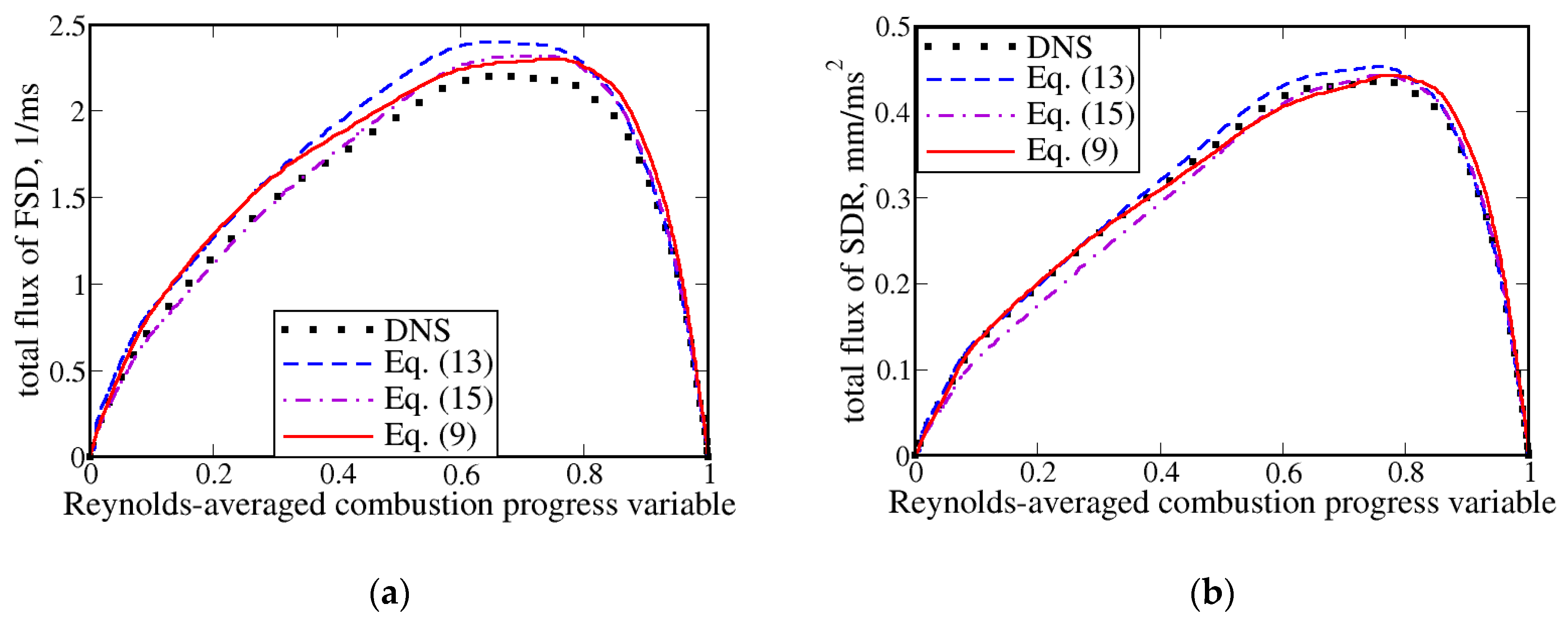
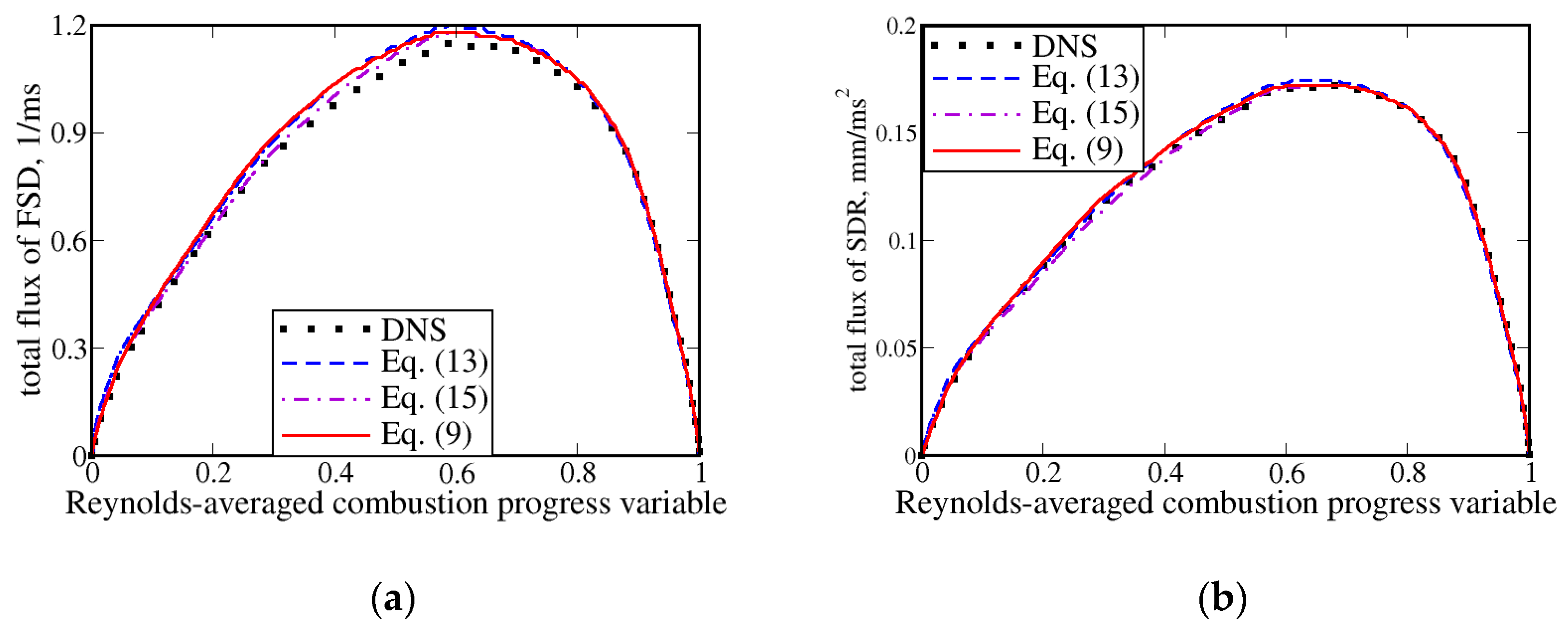
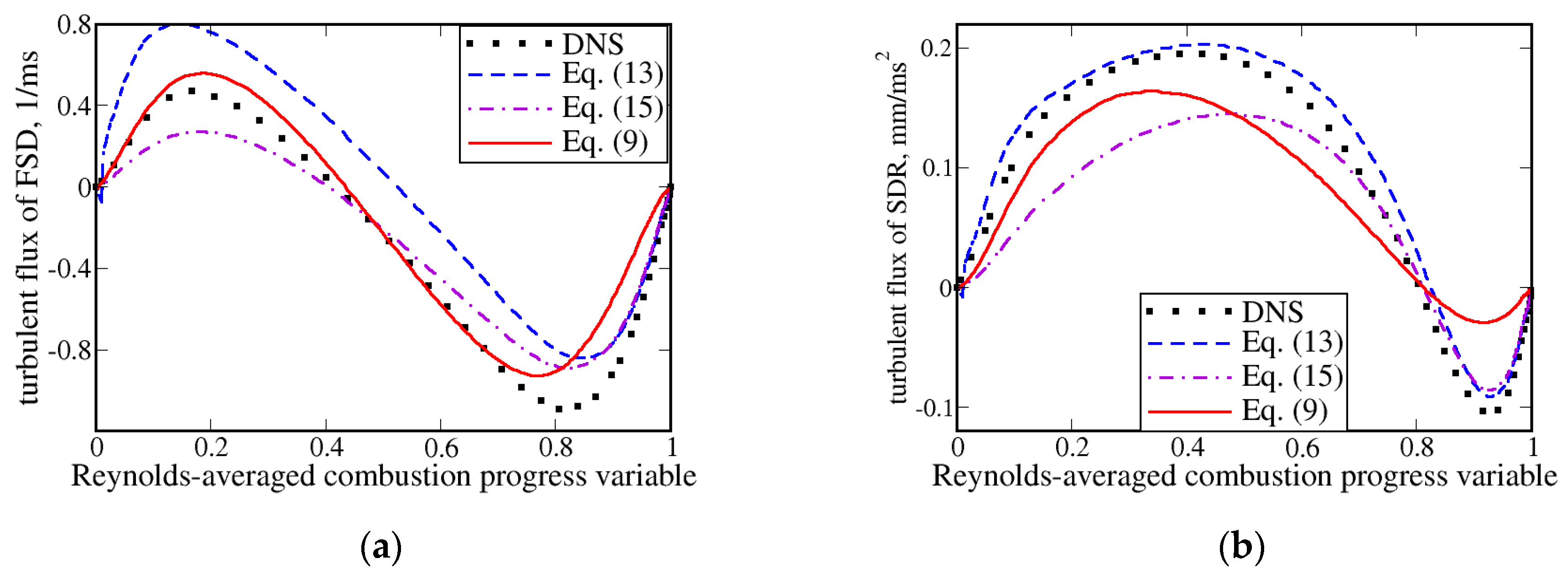
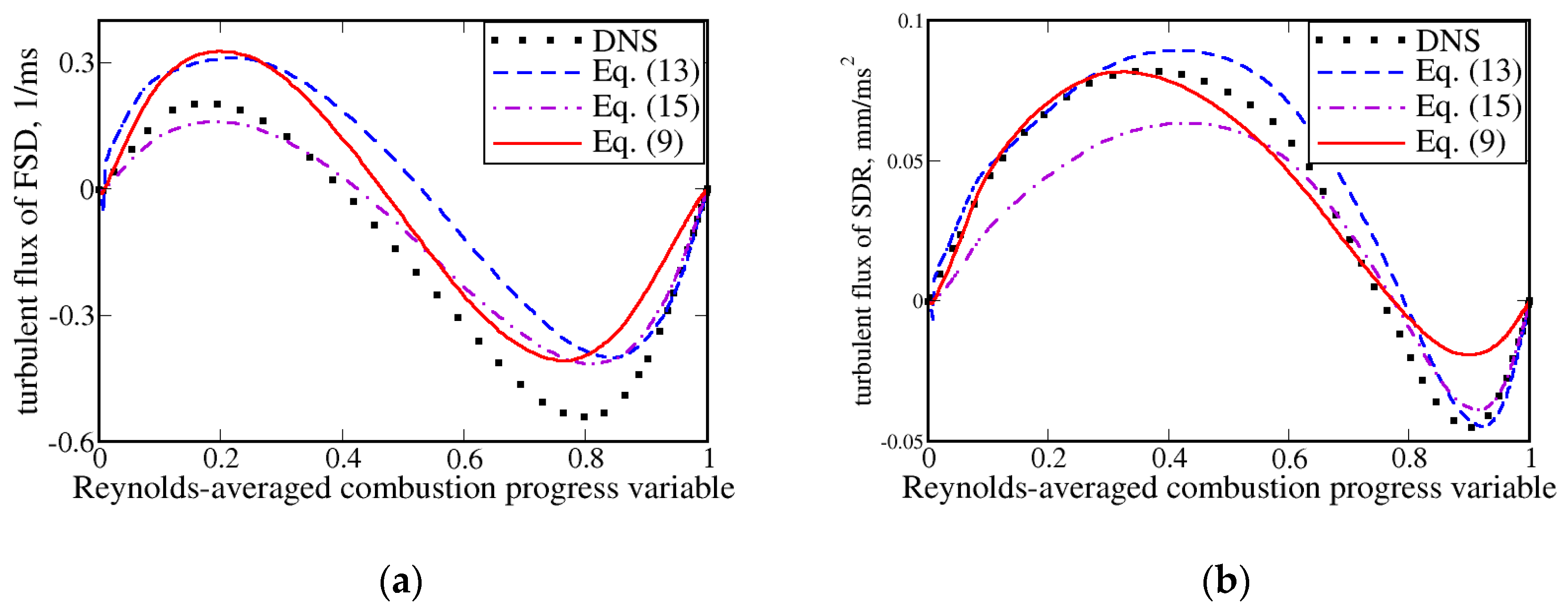
3. Results and Discussion

Results of the developed simple model validation are reported in Figure 1, Figure 2, Figure 3, Figure 4, Figure 5 and Figure 6. Dotted lines in Figure 1a, Figure 2a, and Figure 3a show the total axial FSD flux 〈uΣ〉 extracted directly from the DNS data, whereas solid lines show the flux 〈u〉_f,Σ〈Σ〉 computed using the model, that is, Equations (1) and (9), with 〈c〉^~, 〈u〉^~, 〈ρu″c″〉, and 〈Σ〉 being extracted from the same DNS data. In all three cases H, M, and L, the agreement between the DNS and model results is very good. Similarly, Figure 1b, Figure 2b, and Figure 3b show the total axial SDR flux 〈ρuχ〉 extracted directly from the DNS data, whereas solid lines show the flux 〈u〉_f,χ〈ρχ〉 computed using the model, that is, Equations (2) and (9), with 〈c〉^~, 〈u〉^~, 〈ρu″c″〉, and 〈ρχ〉 being extracted from the same DNS data. Again, the model is well validated in all three cases.

It is worth noting, however, that the magnitudes of the total fluxes 〈uΣ〉 and 〈ρuχ〉 can mainly be controlled by the mean advection fluxes 〈u〉〈Σ〉 and 〈ρ〉〈u〉^~〈χ〉^~, respectively, which do not require modeling. Accordingly, to better access Equation (9), turbulent fluxes were also evaluated as follows:

〈u′Σ′〉 = 〈uΣ〉 − 〈u〉〈Σ〉,

(11)

〈ρu″χ″〉 = 〈ρuχ〉 − 〈ρ〉〈u〉^~〈χ〉^~.

(12)

Results plotted in Figure 4, Figure 5 and Figure 6 show that Equation (9) predicts the axial turbulent fluxes 〈u′Σ′〉 and 〈ρu″χ″〉 very well in the largest parts of mean flame brushes, that is, at 〈c〉 < 0.8, in cases H and M, respectively, cf. dotted and solid lines in Figure 4a and Figure 5b, respectively. Moreover, the flux 〈ρu″χ″〉 is well predicted in case L (see Figure 6b), whereas the peak value of the flux is slightly overestimated. As far as flux 〈u′Σ′〉 in cases M and L or flux 〈ρu″χ″〉 in case H is concerned, Equation (9) yields qualitatively correct results, but some quantitative differences between them and the DNS data are observed, probably due to a simplified treatment of the effects of density variations and finite flamelet thickness in Equations (4) and (5). Nevertheless, these differences do not impede quantitatively predicting the total fluxes 〈u〉〈Σ〉 and 〈ρ〉〈u〉^~〈χ〉^~, in particular, because 〈uΣ〉 is close to the mean flux 〈u〉〈Σ〉 in cases M and L, cf. scales of ordinate axes in Figure 2a or Figure 3a and in Figure 5a or Figure 6a, respectively.

It is worth stressing that the turbulent axial fluxes 〈u′Σ′〉 and 〈ρu″χ″〉 show the countergradient behavior in all studied cases (i.e., 〈u′Σ′〉d〈Σ〉/dx > 0 and 〈ρu″χ″〉d〈ρχ〉/dx > 0), because d〈Σ〉/dx and d〈ρχ〉/dx are positive (negative) in the leading (trailing) part of the mean flame brushes (reactants on the left side). Consequently, the widely used concept of gradient diffusion yields wrong direction of the fluxes 〈u′Σ′〉 and 〈ρu″χ″〉 under conditions of the present DNSs.

It is also worth noting that an alternative model for evaluating the flamelet-conditioned velocity 〈u〉_f was suggested by Bidaux and Bray in an unpublished work (1994) and was subsequently used by Veynante et al. [37]. The model consists in the following linear interpolation:

〈u〉_f = (1 − K)〈u〉_u + K〈u〉_b,

(13)

where the constant K could “be related to the iso-c line used to define the flame location” [37]. Equations (7), (8), and (13) yield

〈u〉_f = 〈u〉^~ + (K − 〈c〉^~)〈ρu″c″〉/[〈ρ〉〈c〉^~(1 − 〈c〉^~)].

(14)

In the cited paper, the constant K was set equal to 0.5 and we are not aware of any alternative suggestion for K. If K = 0.5, Equation (14) can be rewritten in the following form:

〈u〉_f = 〈u〉^~ + (ρ_u/2〈ρ〉)(1 − 2〈c〉^~)〈ρu″c″〉/[ρ_u〈c〉^~(1 − 〈c〉^~)],

(15)

which is similar to Equation (9), but the last term on the right-hand side (RHS) of Equation (15) is multiplied by a factor of R = ρ_u/2〈ρ〉. This factor tends to 1/2 and σ/2 at the leading and trailing edges of the mean flame brush. It is equal to unity somewhere in the middle of the mean flame brush.

While Equations (13)–(15) were never applied to model turbulent fluxes of FSD and SDR, to the best of our knowledge, this gap can easily be filled by assuming that 〈u〉_f,Σ = 〈u〉_f,χ = 〈u〉_f and using Equations (1) or (2), (11) or (12), and (13)–(15). The outcomes of such tests of the model by Bidaux and Bray with K = 0.5 are shown in dashed and dotted-dashed lines in Figure 1, Figure 2, Figure 3, Figure 4, Figure 5 and Figure 6. There are some differences between the results computed using Equations (13) and (15), because Equation (15) is obtained from Equation (13) using Equations (7) and (8), which are exact only in the case of an infinitely thin flame front. In the present DNSs, flamelets have finite thicknesses and, consequently, there are some (sufficiently small) differences between the left-hand side and right-hand side of Equation (7) or (8), extracted from the DNS data (e.g., see Figure 3b in Reference [25]).

The comparison of Equation (13) with Equation (9) shows that Equation (13) with K = 0.5 yields better results for flux 〈ρu″χ″〉 in case H (see Figure 4b), but worse results for flux 〈u′Σ′〉 in cases H and M (see Figure 4a and Figure 5a). Similarly, when compared to Equation (9), Equation (15) yields better results for flux 〈u′Σ′〉 in cases M and L (see Figure 5a and Figure 6a), but worse results for both 〈u′Σ′〉 and 〈ρu″χ″〉 in case H, see Figure 4. Moreover, for both fluxes, Equation (9) is superior to Equation (13) or (15) at the leading edge of the mean flame brush (i.e., at 〈c〉→0). For instance, Equation (15) yields wrong direction of the fluxes at very low 〈c〉 in cases H and M, whereas Equation (13) underestimates the magnitudes |〈u′Σ′〉| and |〈ρu″χ″〉| at very low 〈c〉 in all cases. This difference between Equation (9) and Equation (13) or (15) appears to be of paramount importance, because the leading edge of premixed turbulent flame brush can play the crucial role in its propagation, as discussed in detail elsewhere [38,39,40,41,42,43,44,45]. Furthermore, Equation (13) or (15) yields the same wrong limit behavior of 〈u〉_f→〈u〉_u/2 + 〈u〉_b/2, both at the leading and trailing edges of the mean flame brush in the simplest case of the propagation of an infinitely thin, dynamically passive front in the constant-density turbulent flow. On the contrary, in such a case, Equation (9) obtained in the present work (i) reduces to Equation (3), which was well validated in Reference [14], and (ii) yields 〈u〉_f→〈u〉_b and 〈u〉_f→〈u〉_u at 〈c〉→0 and 〈c〉→1, respectively, in line with the simple physical reasoning discussed at the beginning of Section 2.1.

4. Conclusions

In this study, closure relations for total and turbulent fluxes of flame surface density Σ and scalar dissipation rate χ were developed. The relations did not involve a tuning parameter, very well predicted the total axial fluxes 〈uΣ〉 and 〈ρuχ〉, and reasonably well predicted turbulent axial fluxes 〈u′Σ′〉 and 〈ρu″χ″〉 in three flames characterized by significantly different density ratios and associated with (i) the flamelet regime of premixed turbulent burning, (ii) the validity of the FSD and SDR concepts, and (iii) the countergradient turbulent fluxes of Σ and χ. In the case of a constant density, the developed closure relation reduced to Equation (3), which was recently validated under conditions of gradient turbulent transport [14].

References

1. Candel, S.; Veynante, D.; Lacas, F.; Maistret, E.; Darabiha, N.; Poinsot, T. Coherent flame model: Applications and recent extensions. In Advances in Combustion Modeling; Larrouturou, B.E., Ed.; World Scientific: Singapore, 1990; pp. 19–64. [Google Scholar]
2. Cant, S.R.; Pope, S.B.; Bray, K.N.C. Modelling of flamelet surface-to-volume ratio in turbulent premixed combustion. Proc. Combust. Inst. 1990, 23, 809–815. [Google Scholar] [CrossRef]
3. Borghi, R. Turbulent premixed combustion: Further discussions of the scales of fluctuations. Combust. Flame 1990, 80, 304–312. [Google Scholar] [CrossRef]
4. Veynante, D.; Vervisch, L. Turbulent combustion modeling. Prog. Energy Combust. Sci. 2002, 28, 193–266. [Google Scholar] [CrossRef]
5. Poinsot, T.; Veynante, D. Theoretical and Numerical Combustion, 2nd ed.; Edwards: Philadelphia, PA, USA, 2005. [Google Scholar]
6. Chakraborty, N.; Champion, M.; Mura, A.; Swaminathan, N. Scalar-dissipation-rate approach. In Turbulent Premixed Flames; Swaminathan, N., Bray, K.N.C., Eds.; Cambridge University Press: Cambridge, UK, 2011; pp. 76–102. [Google Scholar]
7. Moss, J.B. Simultaneous measurements of concentration and velocity in an open premixed turbulent flame. Combust. Sci. Technol. 1980, 22, 119–129. [Google Scholar] [CrossRef]
8. Libby, P.A.; Bray, K.N.C. Countergradient diffusion in premixed turbulent flames. AIAA J. 1981, 19, 205–213. [Google Scholar] [CrossRef]
9. Bray, K.N.C. Turbulent transport in flames. Proc. R. Soc. Lond. A 1995, 451, 231–256. [Google Scholar] [CrossRef]
10. Lipatnikov, A.N.; Chomiak, J. Effects of premixed flames on turbulence and turbulent scalar transport. Prog. Energy Combust. Sci. 2010, 36, 1–102. [Google Scholar] [CrossRef]
11. Sabelnikov, V.A.; Lipatnikov, A.N. Recent advances in understanding of thermal expansion effects in premixed turbulent flames. Annu. Rev. Fluid Mech. 2017, 49, 91–117. [Google Scholar] [CrossRef]
12. Bray, K.N.C. Turbulent flows with premixed reactants. In Turbulent Reacting Flows; Libby, P.A., Williams, F.A., Eds.; Springer-Verlag: Berlin, Germany, 1980; pp. 115–183. [Google Scholar]
13. Lipatnikov, A.N. Conditionally averaged balance equations for modeling premixed turbulent combustion in flamelet regime. Combust. Flame 2008, 152, 529–547. [Google Scholar] [CrossRef]
14. Yu, R.; Bai, X.-S.; Lipatnikov, A.N. A direct numerical simulation study of interface propagation in homogeneous turbulence. J. Fluid Mech. 2015, 772, 127–164. [Google Scholar] [CrossRef]
15. Nishiki, S.; Hasegawa, T.; Borghi, R.; Himeno, R. Modeling of flame-generated turbulence based on direct numerical simulation databases. Proc. Combust. Inst. 2002, 29, 2017–2022. [Google Scholar] [CrossRef]
16. Nishiki, S.; Hasegawa, T.; Borghi, R.; Himeno, R. Modelling of turbulent scalar flux in turbulent premixed flames based on DNS databases. Combust. Theory Model. 2006, 10, 39–55. [Google Scholar] [CrossRef]
17. Im, Y.H.; Huh, K.Y.; Nishiki, S.; Hasegawa, T. Zone conditional assessment of flame-generated turbulence with DNS database of a turbulent premixed flame. Combust. Flame 2004, 137, 478–488. [Google Scholar] [CrossRef]
18. Mura, A.; Tsuboi, K.; Hasegawa, T. Modelling of the correlation between velocity and reactive scalar gradients in turbulent premixed flames based on DNS data. Combust. Theory Model. 2008, 12, 671–698. [Google Scholar] [CrossRef]
19. Mura, A.; Robin, V.; Champion, M.; Hasegawa, T. Small scale features of velocity and scalar fields in turbulent premixed flames. Flow Turbul. Combust. 2009, 82, 339–358. [Google Scholar] [CrossRef]
20. Robin, V.; Mura, A.; Champion, M.; Hasegawa, T. Modeling of the effects of thermal expansion on scalar turbulent fluxes in turbulent premixed flames. Combust. Sci. Technol. 2010, 182, 449–464. [Google Scholar] [CrossRef]
21. Robin, V.; Mura, A.; Champion, M. Direct and indirect thermal expansion effects in turbulent premixed flames. J. Fluid Mech. 2011, 689, 149–182. [Google Scholar] [CrossRef]
22. Bray, K.N.C.; Champion, M.; Libby, P.A.; Swaminathan, N. Scalar dissipation and mean reaction rates in premixed turbulent combustion. Combust. Flame 2011, 158, 2017–2022. [Google Scholar] [CrossRef]
23. Lipatnikov, A.N.; Nishiki, S.; Hasegawa, T. A direct numerical simulation study of vorticity transformation in weakly turbulent premixed flames. Phys. Fluids 2014, 26, 105104. [Google Scholar] [CrossRef] [Green Version]
24. Lipatnikov, A.N.; Sabelnikov, V.A.; Nishiki, S.; Hasegawa, T.; Chakraborty, N. DNS assessment of a simple model for evaluating velocity conditioned to unburned gas in premixed turbulent flames. Flow Turbul. Combust. 2015, 94, 513–526. [Google Scholar] [CrossRef]
25. Lipatnikov, A.N.; Nishiki, S.; Hasegawa, T. DNS assessment of relation between mean reaction and scalar dissipation rates in the flamelet regime of premixed turbulent combustion. Combust. Theory Model. 2015, 19, 309–328. [Google Scholar] [CrossRef]
26. Lipatnikov, A.N.; Chomiak, J.; Sabelnikov, V.A.; Nishiki, S.; Hasegawa, T. Unburned mixture fingers in premixed turbulent flames. Proc. Combust. Inst. 2015, 35, 1401–1408. [Google Scholar] [CrossRef]
27. Sabelnikov, V.A.; Lipatnikov, A.N.; Chakraborty, N.; Nishiki, S.; Hasegawa, T. A transport equation for reaction rate in turbulent flows. Phys. Fluids 2016, 28, 081701. [Google Scholar] [CrossRef] [Green Version]
28. Sabelnikov, V.A.; Lipatnikov, A.N.; Chakraborty, N.; Nishiki, S.; Hasegawa, T. A balance equation for the mean rate of product creation in premixed turbulent flames. Proc. Combust. Inst. 2017, 36, 1893–1901. [Google Scholar] [CrossRef]
29. Lipatnikov, A.N.; Sabelnikov, V.A.; Nishiki, S.; Hasegawa, T. Flamelet perturbations and flame surface density transport in weakly turbulent premixed combustion. Combust. Theory Model. 2017, 21, 205–227. [Google Scholar] [CrossRef]
30. Lipatnikov, A.N.; Sabelnikov, V.A.; Chakraborty, N.; Nishiki, S.; Hasegawa, T. A DNS study of closure relations for convection flux term in transport equation for mean reaction rate in turbulent flow. Flow Turbul. Combust. 2018, 100, 75–92. [Google Scholar] [CrossRef] [PubMed]
31. Lipatnikov, A.N.; Chomiak, J.; Sabelnikov, V.A.; Nishiki, S.; Hasegawa, T. A DNS study of the physical mechanisms associated with density ratio influence on turbulent burning velocity in premixed flames. Combust. Theory Model. 2018, 22, 131–155. [Google Scholar] [CrossRef]
32. Lipatnikov, A.N.; Sabelnikov, V.A.; Nishiki, S.; Hasegawa, T. Combustion-induced local shear layers within premixed flamelets in weakly turbulent flows. Phys. Fluids 2018, 30, 085101. [Google Scholar] [CrossRef]
33. Lipatnikov, A.N.; Sabelnikov, V.A.; Nishiki, S.; Hasegawa, T. Does flame-generated vorticity increase turbulent burning velocity? Phys. Fluids 2018, 30, 081702. [Google Scholar] [CrossRef]
34. Sabelnikov, V.A.; Lipatnikov, A.N.; Nishiki, S.; Hasegawa, T. Application of conditioned structure functions to exploring influence of premixed combustion on two-point turbulence statistics. Proc. Combust. Inst. 2019, 37, 2433–2441. [Google Scholar] [CrossRef]
35. Lipatnikov, A.N.; Nishiki, S.; Hasegawa, T. A DNS assessment of linear relations between filtered reaction rate, flame surface density, and scalar dissipation rate in a weakly turbulent premixed flame. Combust. Theory Model. 2019, 23. [Google Scholar] [CrossRef]
36. Sabelnikov, V.A.; Lipatnikov, A.N.; Nishiki, S.; Hasegawa, T. Investigation of the influence of combustion-induced thermal expansion on two-point turbulence statistics using conditioned structure functions. J. Fluid Mech. 2019, in press. [Google Scholar]
37. Veynante, D.; Trouvé, A.; Bray, K.N.C.; Mantel, T. Gradient and counter-gradient scalar transport in turbulent premixed flames. J. Fluid Mech. 1997, 332, 263–293. [Google Scholar] [CrossRef]
38. Kuznetsov, V.R.; Sabelnikov, V.A. Turbulence and Combustion; Hemisphere Publishing Corporation: New York, NY, USA, 1990. [Google Scholar]
39. Lipatnikov, A.N.; Chomiak, J. Molecular transport effects on turbulent flame propagation and structure. Prog. Energy Combust. Sci. 2005, 31, 1–73. [Google Scholar] [CrossRef]
40. Lipatnikov, A.N. Fundamentals of Premixed Turbulent Combustion; CRC Press: Boca Raton, FL, USA, 2012. [Google Scholar]
41. Venkateswaran, P.; Marshall, A.; Seitzman, J.; Lieuwen, T. Scaling turbulent flame speeds of negative Markstein length fuel blends using leading points concepts. Combust. Flame 2015, 162, 375–387. [Google Scholar] [CrossRef]
42. Sabelnikov, V.A.; Lipatnikov, A.N. Transition from pulled to pushed fronts in premixed turbulent combustion: Theoretical and numerical study. Combust. Flame 2015, 162, 2893–2903. [Google Scholar] [CrossRef]
43. Kim, S.H. Leading points and heat release effects in turbulent premixed flames. Proc. Combust. Inst. 2017, 36, 2017–2024. [Google Scholar] [CrossRef]
44. Dave, H.L.; Mohan, A.; Chaudhuri, S. Genesis and evolution of premixed flames in turbulence. Combust. Flame 2018, 196, 386–399. [Google Scholar] [CrossRef]
45. Lipatnikov, A.N.; Chakraborty, N.; Sabelnikov, V.A. Transport equations for reaction rate in laminar and turbulent premixed flames characterized by non-unity Lewis number. Int. J. Hydrog. Energy 2018, 43, 21060–21069. [Google Scholar] [CrossRef]
Figure 1. Total axial fluxes of (a) flame surface density (FSD) Σ and (b) scalar dissipation rate (SDR) χ. Case H.
Fluids 04 00043 g001
Figure 2. Total axial fluxes of (a) FSD Σ and (b) SDR χ. Case M.
Fluids 04 00043 g002
Figure 3. Total axial fluxes of (a) FSD Σ and (b) SDR χ. Case L.
Fluids 04 00043 g003
Figure 4. Turbulent axial fluxes of (a) FSD Σ and (b) SDR χ. Case H.
Fluids 04 00043 g004
Figure 5. Turbulent axial fluxes of (a) FSD Σ and (b) SDR χ. Case M.
Fluids 04 00043 g005
Figure 6. Turbulent axial fluxes of (a) FSD Σ and (b) SDR χ. Case L.
Fluids 04 00043 g006