The Effect of a Variable Background Density Stratification and Current on Oceanic Internal Solitary Waves

Abstract

Large amplitude, horizontally propagating internal waves are commonly observed in the coastal ocean. They are often modelled by a variable-coefficient Korteweg–de Vries equation to take account of a horizontally varying background state. Although this equation is now well-known, a term representing non-conservative effects, arising from horizontal variation in the underlying basic state density stratification and current, has often been omitted. In this paper, we examine the possible significance of this term using climatological data for several typical oceanic sites where internal waves have been observed.

1. Introduction

Large amplitude internal solitary waves are commonly observed in the coastal ocean (see the reviews by Grimshaw [1], Holloway et al. [2], Ostrovsky and Stepanyants [3], Helfrich and Melville [4,5], Grimshaw et al. [6] and the book by Vlasenko et al. [7]). As they are long waves with wavelengths greater than the relevant vertical scale, it is widely accepted that the basic paradigm for the description of these waves is based on the Korteweg–de Vries (KdV) equation, first derived in this context by Benney [8] and Benjamin [9] and subsequently by many others (see the aforementioned references). However, typically, they propagate through regions of horizontally variable density stratification and background currents, and over variable bottom topography. Hence, a variable-coefficient Korteweg–de Vries (vKdV) equation is needed to model these waves. For internal waves, this is given by (see Grimshaw [10], Zhou and Grimshaw [11] for a detailed derivation),

$${\eta }_t+c{\eta }_x+\frac{c{Q}_x}{2Q}\eta +\mu \eta {\eta }_x+\delta {\eta }_{xxx}+\sigma \eta +\mathcal{D}\left(\eta \right)=0.$$

(1)

Here, $\eta (x,t)$ is the internal wave amplitude of the relevant modal function, usually mode 1 (see Section 2 for a precise definition). In (1), $x,t$ are space and time variables, $c\left(x\right)$ is the relevant linear long wave speed, and $Q\left(x\right)$ is the linear magnification factor, defined so that $Q{\eta }^2$ is the wave action flux density for linear long waves. The coefficients $c,Q,\mu ,\delta ,\sigma$ are slowly-varying functions of x and are determined by the relevant waveguide properties. $\mathcal{D}\left(\eta \right)$ is a frictional term, which can take various forms (see the aforementioned review articles). For most of this paper, we omit this term, but we will return to it later in Appendix A. Formally, the derivation requires the usual KdV scaling where $\eta \sim {ϵ}^2$, $\partial /\partial x\sim ϵ$, $\partial /\partial t\sim ϵ$. Then, the first two terms in (1) are the dominant terms and the evolution takes place on a spatial scale $x\sim {ϵ}^{-3}$. The coefficients $c,Q,\mu ,\delta$ vary on this same spatial scale $x\sim {ϵ}^{-3}$, while $\sigma \sim {ϵ}^3$ and $\mathcal{D}\left(\eta \right)\sim {ϵ}^5$.

Our main concern in this paper is with the term $\sigma \eta$, which represents non-conservative effects arising from the horizontal variability in the underlying basic state density stratification and current. An outline of the derivation of (1) was given by Liu et al. [12] and for convenience is briefly summarised here in Section 2, emphasising how the “new” term $\sigma \eta$ arises. It is present because the vKdV Equation (1) describes the evolution of a wave field about a basic state which may not be in exact equilibrium due to the inhomogeneous background state. That is, it does not satisfy the underlying conservative full equation set, in this case the two-dimensional Euler equations, which can be constructed from a Lagrangian. Andrews and McIntyre [13], Grimshaw [14], have described in a general context how this term arises when considering wave action conservation. We use the term “non-conservative” here and throughout in the restricted sense that it is non-conservative only because the horizontal variability of the basic state current and density fields, taken from oceanic data, may not satisfy the two-dimensional Euler equations. Note that the horizontal variation of the fluid depth h is mainly already accounted for in the linear magnification factor Q, and ensures that the wave action flux $Q{\eta }^2$ is conserved in the conservative case. Although the “new” term has the form of Rayleigh friction, importantly this term has no connection with dissipative processes on the internal waves themselves. Unlike the usual Rayleigh friction, $\sigma$ varies with distance, can be positive or negative, and indeed can change sign along the wave path. Although this term has been known for over three decades, it has usually been neglected in modelling studies. Zhou and Grimshaw [11] examined some possible scenarios of how the term might arise, and, recently in Liu et al. [12], we examined its effect for a model two-layer fluid and for three oceanic cases previously considered by Grimshaw et al. [15], where the term had been omitted. In this paper, we use climatological data from five typical oceanic sites where internal waves have been observed. Importantly, we also now include a background current, which was of necessity omitted in Liu et al. [12] because of the lack of suitable current data.

Since the first two terms in (1) are the dominant terms, we can make the transformation

$$A=\sqrt{Q}\eta ,T={\int }_0^x\frac{dx}{c},X=T-t.$$

(2)

Substitution into (1) yields, to the same order of asymptotic approximation as in the derivation of (1), and after omitting the dissipation term $\mathcal{D}\left(\eta \right)$ (although we shall return to this later),

$$A_T+\nu A{A}_X+\lambda A_{XXX}+\sigma A=0,$$

(3)

$$\nu =\frac{\mu }{c\sqrt{Q}},\lambda =\frac{\delta }{c^3}.$$

(4)

The coefficients $\nu ,\lambda ,\sigma$ are functions of T alone. In addition, since we can assume $\delta >0$ without loss of generality, we make a further transformation yielding the canonical form,

$$A_{\tau }+\alpha A{A}_X+A_{XXX}+\beta A=0,$$

(5)

$$\mathrm{where}\tau ={\int }_0^T\lambda dT={\int }_0^x\frac{\delta }{c^4}dx,\alpha =\frac{\nu }{\lambda }=\frac{\mu c^2}{\sqrt{Q}\delta },\beta =\frac{\sigma }{\lambda }=\frac{\sigma c^3}{\delta }.$$

(6)

Note that the coefficients $\alpha ,\beta$, originally expressed as functions of x, are now functions of $\tau$ through the transformation $\tau =\tau \left(x\right)$ (6). A further transformation yields the form suitable for numerical simulation,

$$A=R\tilde{A},R=exp(-{\int }_0^{\tau }\beta d{\tau }^{\prime }),{\tilde{A}}_{\tau }+\tilde{\alpha }\tilde{A}{\tilde{A}}_X+{\tilde{A}}_{XXX}=0,\tilde{\alpha }=R\alpha .$$

(7)

The scaling factor R is a cumulative measure of the coefficient $\beta$. In the sequel, we will show some simulations of this equation. There are two conservation laws

$$\begin{array}{ccc}\hfill \frac{\partial M}{\partial \tau }=0,M& =& {\int }_{-\infty }^{\infty }\tilde{A}dX,\hfill \end{array}$$

(8)

$$\begin{array}{ccc}\hfill \frac{\partial P}{\partial \tau }=0,P& =& {\int }_{-\infty }^{\infty }{\tilde{A}}^{2}dX,\hfill \end{array}$$

(9)

relating to mass and wave action flux, respectively.

In Section 2, we present a brief summary of the derivation of (1) emphasising the origin of the coefficient $\sigma$. Then, in Section 3, we present some case studies based on climatological data for five typical oceanic sites. Three of these show that the effect on the “new term” $\sigma \eta$ is measurable but small, while the other two cases are when it is quite significant. We conclude in Section 4. In the Appendix A and Appendix B, we examine the possible effects of bottom friction and the earth’s background rotation, neglected in the main body of the paper.

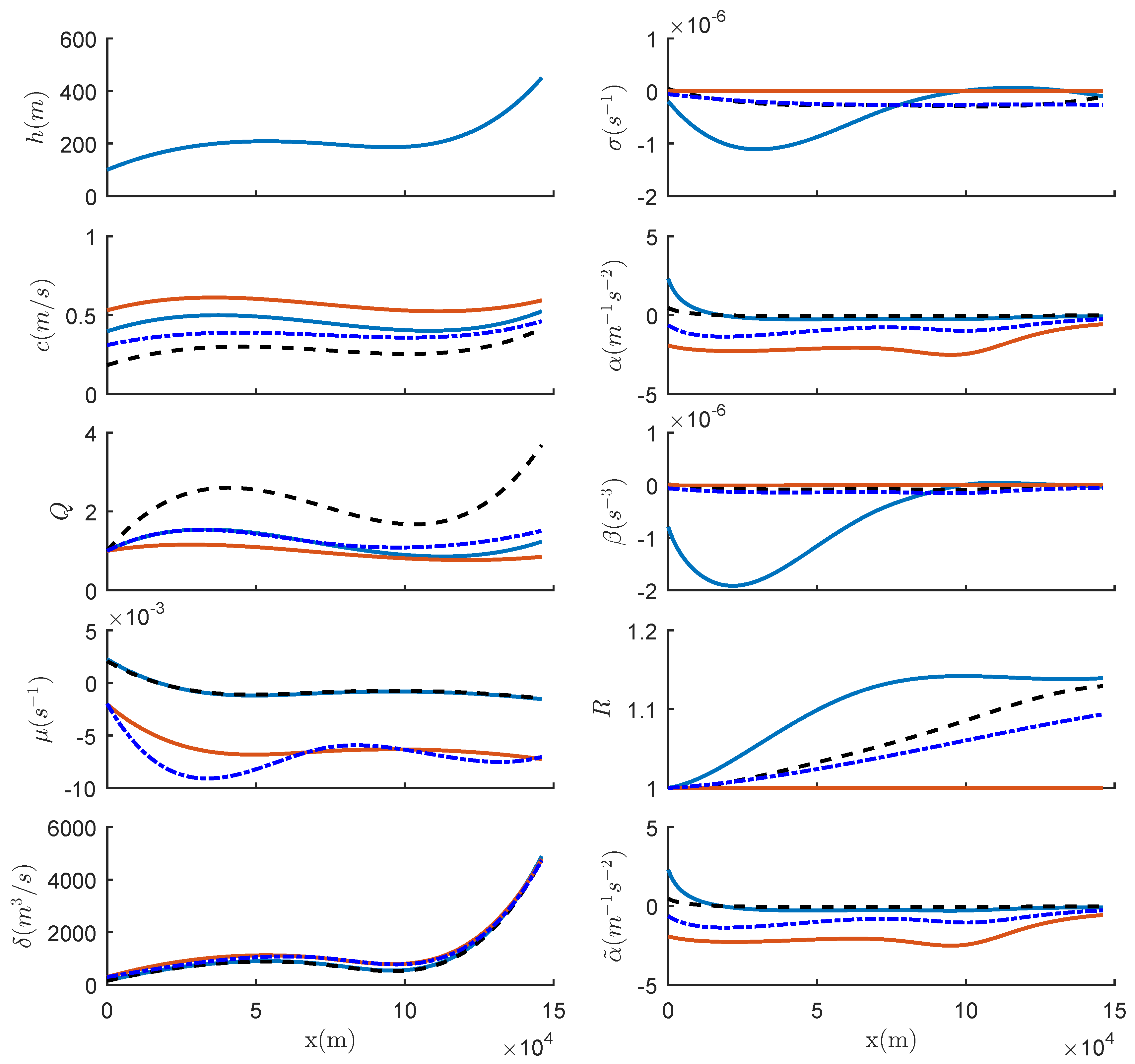
2. Variable-Coefficient Korteweg–De Vries Equation

The vKdV Equation (1) was derived by Grimshaw [10] (see also Zhou and Grimshaw [11]) and was summarised in our previous paper, Liu et al. [12]. That summary is briefly reproduced here for convenience, and also to define the coefficients in (1). We assume a two-dimensional configuration, so that there is no y-dependence in either the basic state or in the wave field. Then, the basic state consists of a depth $h=h\left(x\right)$, a background horizontal current in the wave direction $u_0(z;x)$ with a corresponding vertical velocity field $w_0(z;x)$, a density field ${\rho }_0(z;x)$ with a corresponding pressure field $p_0(z;x)$ and a free surface displacement ${\zeta }_0\left(x\right)$. When the basic current field and density fields have an explicit x-dependence, as may arise in practice when, as here, they are obtained from actual oceanic data, this basic state may not satisfy the full steady-state two-dimensional Euler equations. Hence, body forces $F_0(z;x),G_0(z;x)$ are inserted into the momentum equations, and a source term $H_0(z;x)$ is inserted into the density equation, in order to take account of this. Note that the source term $H_0(z;x)$ was omitted in Liu et al. [12] but is included here to allow for the presence of a background current. Thus, the basic state equations are

$$\begin{array}{ccc}\hfill {\rho }_0(u_0{u}_{0x}+w_0{u}_{0z})+p_{0x}& =& F_0,\hfill \end{array}$$

(10)

$$\begin{array}{ccc}\hfill {\rho }_0(u_0{w}_{0x}+w_0{w}_{0z})]+p_{0z}+g{\rho }_0& =& \left[G_0\right],\hfill \end{array}$$

(11)

$$\begin{array}{ccc}\hfill u_0{\rho }_{0x}+w_0{\rho }_{0z}& =& H_0,\hfill \end{array}$$

(12)

$$\begin{array}{ccc}\hfill u_{0x}+w_{0z}& =& 0,\hfill \end{array}$$

(13)

in the fluid domain $-h<z<{\zeta }_0$. The boundary conditions are

$$\begin{array}{ccc}\hfill w_0+u_0{h}_x& =& 0,\mathrm{at}z=-h\left(x\right),\hfill \end{array}$$

(14)

$$\begin{array}{ccc}\hfill p_0& =& 0,\mathrm{at}z={\zeta }_0,\hfill \end{array}$$

(15)

$$\begin{array}{ccc}\hfill u_0{\eta }_{0x}& =& w_0,\mathrm{at}z={\zeta }_0.\hfill \end{array}$$

(16)

As discussed above, the important issue here is that, due to the observed horizontal inhomogeneity in the background density and current, this background state is not in exact equilibrium, and does not satisfy the two-dimensional inviscid Euler equations. Hence, the terms $F_0(z;x),G_0(z;x)$ and $H_0(z;x)$ are then needed to support the basic state. They may arise from diabatic effects, dissipative effects, Coriolis terms, or driving terms such as wind stress. However, we do not examine the origin of these terms directly. Instead, we use oceanic data to find the background state ${\rho }_0(z;x)$ and $u_0(z;x)$ and hence estimate $F_0(z;x),G_0(z;x)$ and $H_0(z;x)$ directly, without regard to their precise physical origin. We emphasise again that, although these terms may be related to diabatic and dissipative processes in the basic state, they do not have any direct relation to wave dissipation processes per se.

Because the x-dependence is slow, technically $\partial /\partial x\sim {ϵ}^3$, $w_0\sim {ϵ}^3$, $F_0\sim {ϵ}^3$, $H_0\sim {ϵ}^3$ while $G_0\sim {ϵ}^6$, so that the dominant balance in the vertical momentum equation is hydrostatic and the terms in $[·]$ can be omitted. Importantly, note that a transverse velocity field $v_0(z;x)$ and Coriolis term $f{v}_0$ are not included on the left-hand side of (10) and, if present, have been absorbed into the body force term $F_0$ (see Grimshaw [10], Zhou and Grimshaw [11]). In addition, note that, if such terms are present, we have nevertheless ignored any possible slow y-dependence of order ${ϵ}^3$, as this additional complication is beyond the scope of this present study. However, we discuss this issue later at the end of the opening part of Section 3. We have included here an additional source term $H_0$ in (12) to allow for the possibility that the density field is maintained by diabatic effects, through the dependence on the underlying temperature and salinity fields. This extra term leads to a minor modification to the derivation in Grimshaw [10], Zhou and Grimshaw [11]. However, we note that this term is small when the Boussinesq approximation is made (see below).

This basic state is then perturbed by the wave field, where at the leading order the perturbation vertical particle displacement is given by

$$\zeta \sim \eta (x,t)\varphi (z;x).$$

(17)

Here the modal function $\varphi (z;x)$ together with the linear long wave speed $c\left(x\right)$ is defined by the boundary-value problem,

$$\begin{array}{ccc}\hfill {\{{\rho }_0{(c-u_0)}^2{\varphi }_z\}}_z-g{\rho }_{0z}\varphi & =& 0,\mathrm{for}-h<z<{\eta }_0,\hfill \end{array}$$

(18)

$$\begin{array}{ccc}\hfill \varphi =0\mathrm{at}z=-h,{(c-u_0)}^2{\varphi }_z& =& g\varphi \mathrm{at}z={\eta }_0.\hfill \end{array}$$

(19)

In general, there is an infinite set of such modal functions, but here we shall, in the sequel, examine only the lowest internal mode, often designated as mode 1. Continuation of this asymptotic expansion to the next order than yields the vKdV Equation (1) (see Grimshaw [10], Zhou and Grimshaw [11], Liu et al. [12] or the reviews by Grimshaw [5], Grimshaw et al. [6]). The coefficients are given by

$$\begin{array}{ccc}\hfill I\mu & =& 3{\int }_{-h}^{{\eta }_0}{\rho }_0{(c-u_0)}^2{\varphi }_z^{3}dz,\hfill \end{array}$$

(20)

$$\begin{array}{ccc}\hfill I\delta & =& {\int }_{-h}^{{\eta }_0}{\rho }_0{(c-u_0)}^2{\varphi }^{2}dz,\hfill \end{array}$$

(21)

$$\begin{array}{ccc}\hfill \mathrm{where}I& =& 2{\int }_{-h}^{{\eta }_0}{\rho }_0(c-u_0){\varphi }_z^{2}dz,Q=c^{2}I,\hfill \\ \hfill \mathrm{and}I\sigma & =& -{\int }_{-h}^{{\eta }_0}\varphi {\varphi }_z{K}_{0z}dz,\hfill \end{array}$$

(22)

$$\begin{array}{ccc}\hfill K_0& =& F_0+u_0{H}_0=u_0{\left({\rho }_0{u}_0\right)}_x+w_0{\left({\rho }_0{u}_0\right)}_z+p_{0x}.\hfill \end{array}$$

(23)

These expressions are all well-known, except for the coefficient $\sigma$ which represents non-conservative effects (see Grimshaw [10], Zhou and Grimshaw [11], Liu et al. [12] for the case when $H_0=0$). That case can be extended to the situation here when $H_0\ne 0$, or this term can also be obtained in full directly from the general theory for wave action when there are non-conservative terms (see Grimshaw [14]).

3. Estimation of the Non-Conservative Term from Oceanic Data

The primary purpose of this paper is to examine the possible significance of the non-conservative term with coefficient $\sigma$ in (1) or $\beta$ in the transformed Equation (5). For this purpose, we examined three latitudinal and two longitudinal transects (see Figure 1) of the coastal ocean where internal solitary waves are known to occur frequently, these being on the West Coast of Portugal (WP), in the South China Sea (SCS), on the North West Shelf of Australia (NWS), along the Malvinas Current (MC) and near the Amazon River mouth (ARM). In each case, we use the oceanic data to evaluate the coefficient $\sigma$ and then test through numerical simulations how much influence this term might have on the propagation of internal waves in each of these cases. For this purpose, we use monthly-mean climatological data provided from NOAA. The spatial resolution of this data is $0.333$ degrees in latitude and $1.0$ degrees in longitude. A global grid ($418\times 360$) spans from 74.5 S–64.5 N, 0.5 E–359.5 E and the vertical levels (40 in total) go from 5 to 4478 m depth. For our numerical simulations of the vKdV Equation (5), we choose data in two summer months (July and August, 2005) and two winter months (January and February, 2006). Note that we call July and August ‘summer’ and January and February ‘winter’, no matter if it is in the northern or southern hemisphere. From this data, we obtain the modal function (18) and all the vKdV coefficients (20)–(23) both with and without a basic background current $u_0$, that is for both $H_0\ne 0$, $H_0=0$. Note that, consistent with the basic theory, we take $u_0$ to be the current along the transect, and ignore the component normal to the transect. The KdV coefficients and the transformed coefficients in (6) for each transect are displayed in the following subsections, together with some numerical simulations of the vKdV Equation (5). In the simulations, $\alpha$, $\beta$, R and $\tilde{\alpha }$ are non-dimensional with a length scale of 100 m and a velocity scale of 1 m s⁻¹, respectively.

For each latitudinal transect, we have data ${\rho }_0(z;i)$ and $u_0(z;i)$ at sites $i=1,2\cdots n$ where typically we choose $n=5$. From these, we compute the modal function $\varphi (z;i)$, and the speed $c\left(i\right)$, and hence the nonlinear coefficient $\mu \left(i\right)$ (20), the dispersive coefficient $\delta \left(i\right)$ (21) and $Q\left(i\right)$ (22). Then, we use a spline interpolation to get $c\left(x\right),\mu \left(x\right),\delta \left(x\right),Q\left(x\right)$. To find an expression for $\sigma$ (23), we need expressions for $u_{0x}$ and ${\rho }_{0x}$. First, we note that it is useful here to use the Boussinesq approximation and the rigid lid approximation, so that (23) becomes

$$I\sigma \approx -{\int }_{-h}^{{\eta }_0}(u_0{u}_{0x}+w_0{u}_{0z}){\rho }_0({\varphi }_z^2+\varphi {\varphi }_{zz})dz+{\int }_{-h}^{{\eta }_0}\varphi {\varphi }_{z}g{\rho }_{0x}dz.$$

(24)

Here, the first term arises after integration by parts, and in the second term we have used hydrostatic balance so that $p_{0zx}=-g{\rho }_{0x}$. Note that the outcome for $\sigma$ in (24) is the same as if we set $H_0=0$ in (23) indicating that as anticipated, the term $H_0$ is very small when the Boussinesq approximation is made.

To get ${\rho }_{0x}(z;x),$ we first interpolate ${\rho }_0(z;i)$ to get ${\rho }_0(z;x)$ as above, and the depth $h_i$ is likewise interpolated to $h\left(x\right)$. However, a difficulty now arises as ${\rho }_0(z;i)$ is defined in a variable domain $-h\left(i\right)<z<0$, and hence the interpolation procedure depends on the index i. To illustrate how this can be overcome, we suppose that $n=5$, that is, $i=1,2,3,4,5$. For the usual case of a decreasing depth, we can assume that $h_5>h_4>h_3>h_2>h_1$. Then, interpolation for five sites is done for each fixed z in the range $0>z>-h_1$, for four sites $-h_1>z>-h_2$, and so on, but cannot be done in the bottom layer $-h_4>z>-h_5$. We assign ${\rho }_0(z;x)$ in the bottom layer at site $i=5$ to be the same value as in the fourth layer. Thus, ${\rho }_{0x}(z;x)$ is a cubic, quadratic and linear function of x in the top, second and third layer, respectively, a constant in the fourth and fifth layer. The estimation of $u_{0x}$ is analogous.

Importantly, we note that, although the real oceanic background flow fields may be three-dimensional, the transects we choose are two-dimensional along the assumed wave propagation direction. In particular, as discussed above, our developed theory ignores any possible y-dependence in the basic state, and in particular does not take account of a term $v_{0y}$ in the incompressibility condition (13). This is permissible along a strong unidirectional current, such as a tidal flow or boundary current, or possibly even along the axis of an oceanic eddy. The data we examine do show that $v_0\ne 0$, but we cannot determine $v_{0y}$ from our transect, and the quality of the data does not allow us to check $w_{0z}$ to see the actual balance in the incompressibility condition (13). Since the theory is two-dimensional, we replace $w_{0z}$ by $-u_{0x}$ in Equation (24) (see Equation (13)) because the quality of $w_0$ is not good enough to find $w_{0z}$ with sufficient accuracy.

Available in situ oceanic data on transects where internal waves have been recorded typically show horizontal gradients in ${\rho }_0$ and, although the corresponding data for $u_0$ is sometimes absent, we suspect it will also be horizontally varying. If $u_0$ does vary with x, then $w_0$ must be nonzero in the two-dimensional theory we are using, but it is very small as can be seen in the results we present below. Note that in our previous paper Liu et al. [12], we set $u_0=0$ and $w_0=0$, but $\sigma \ne 0$ due to the observed horizontal density stratification. We present these five cases in two parts. In the first part with three cases, even though $u_0\ne 0$, we find that the horizontal density stratification was the major contribution to $\sigma$. In these first three cases, although the effect of the term $\sigma \eta$ on the wave field is measurable, the impact of including this new term is quite small. However, in the second part with two cases, the contribution from $u_0$ was significant, and we find that the new term has a significant impact on the evolution of the wave field.

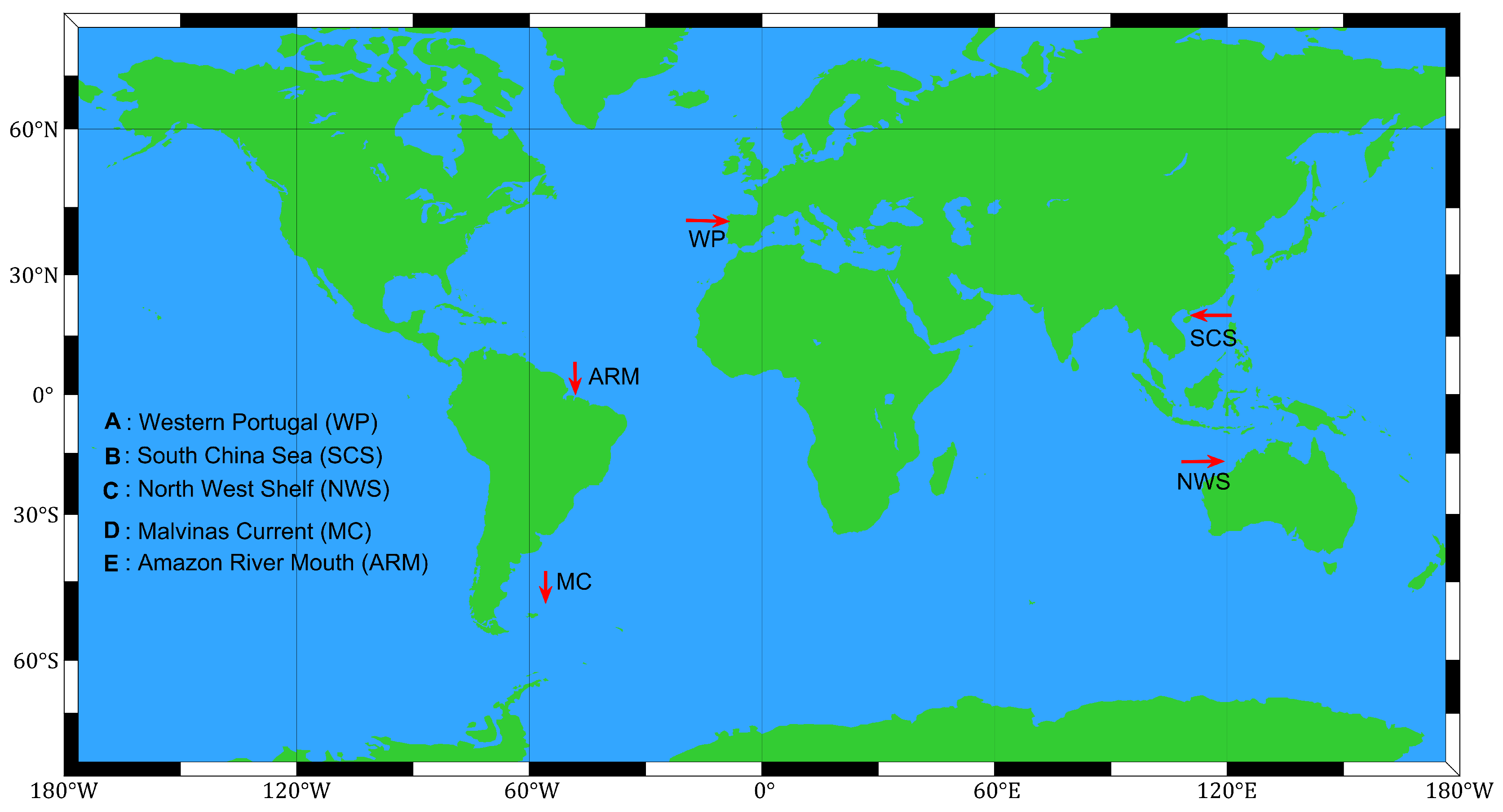
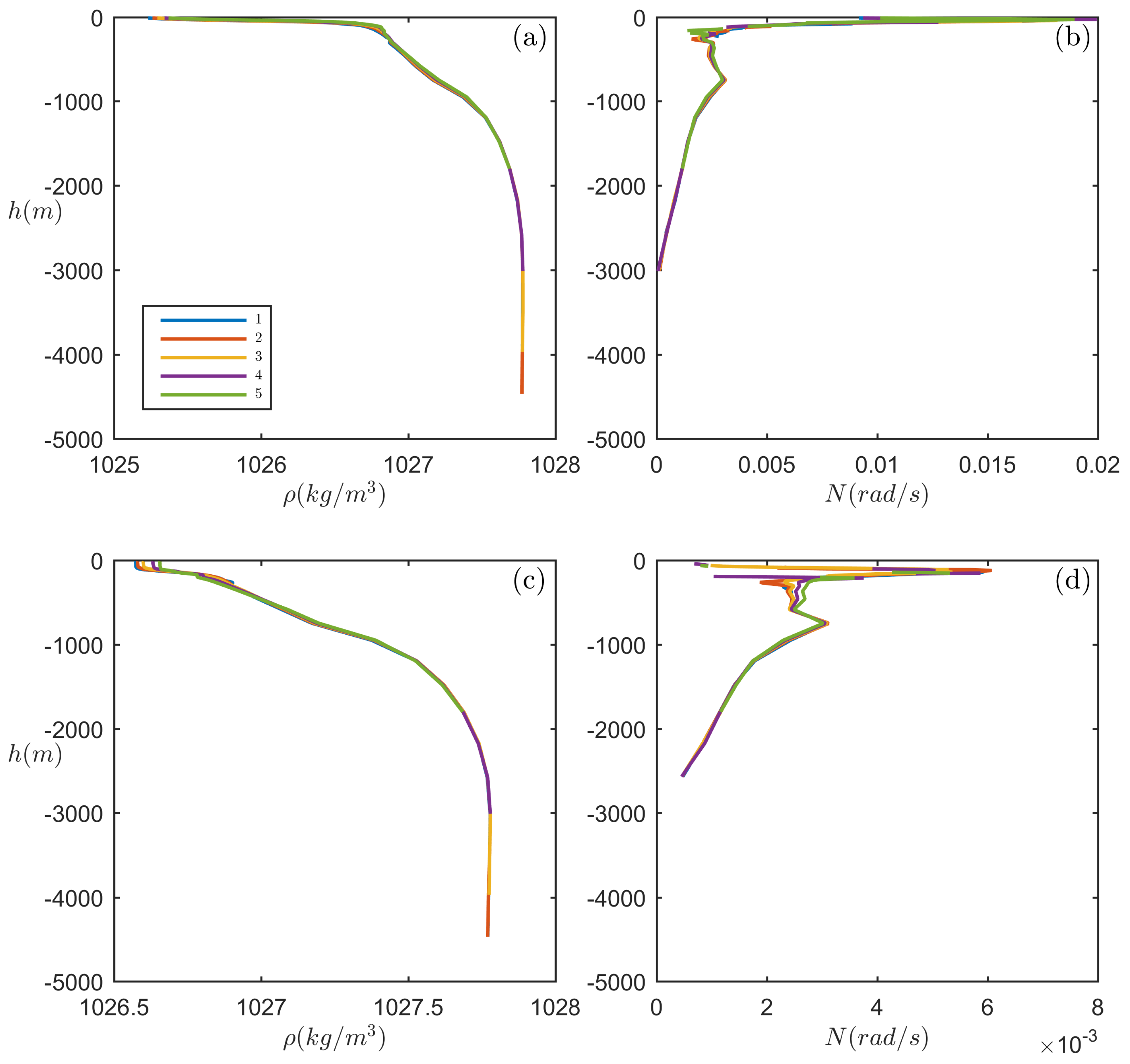
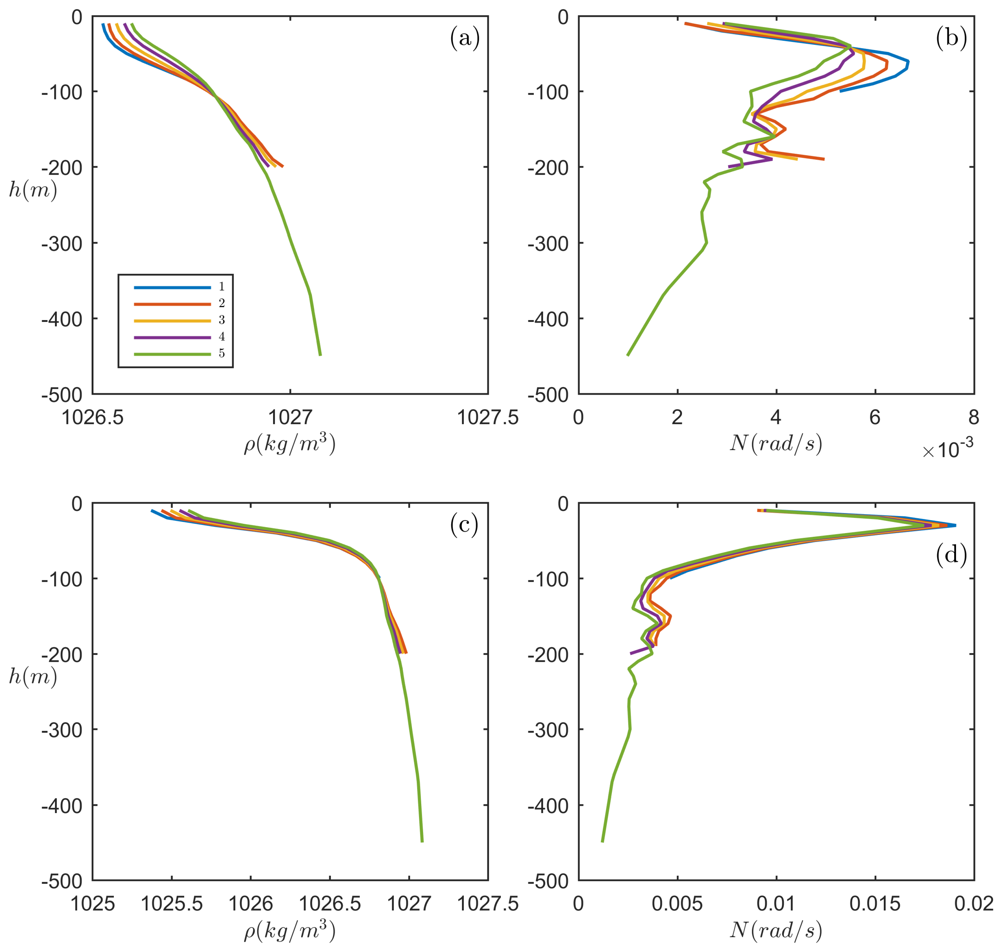
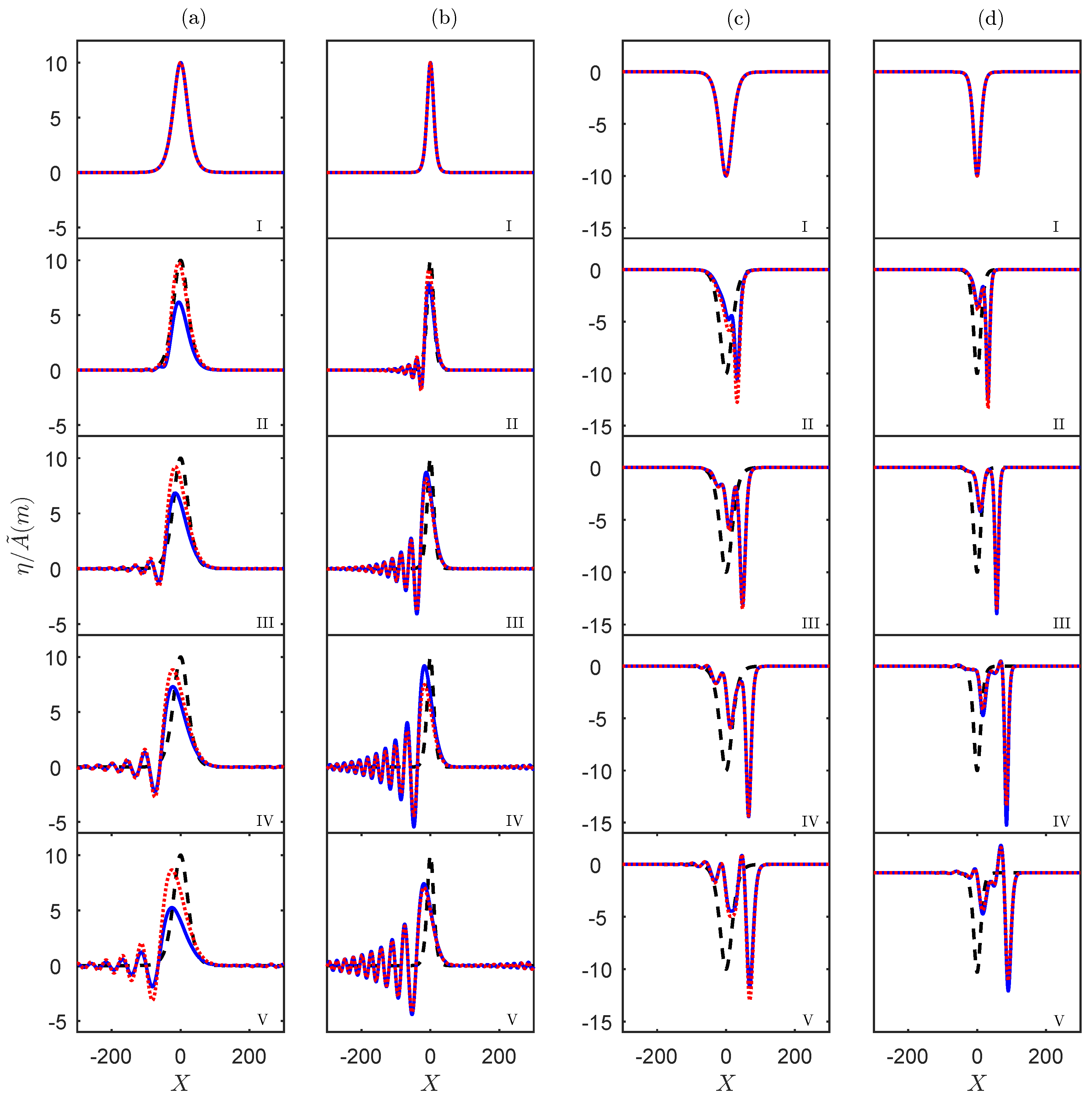
3.1. Cases Where the Horizontal Density Stratification Is the Major Effect

3.1.1. A: Western Portugal

Here, we choose a transect close to Western Portugal along a latitude from the point 38.50 N, 14.5 W to the point 38.50 N, 10.5 W. The water depth varies from 4470 m to 1800 m on the continental slope off western Portugal. Figure 2 shows the background density field at five points along the transect. We see that there is variability along the transect, especially noticeable in the buoyancy frequency near the pycnocline, and larger in winter than in summer. It can be treated as an approximate two-layer stratification with a top layer thinner than the bottom, which indicates that there is no polarity change; here, $\mu <0,\alpha <0$ as shown in Figure 3. From the vKdV coefficients shown in Figure 3, we see that $\left|\alpha \right|$ increases shorewards as the depth decreases, indicating that the effect of nonlinearity increases. The background current $u_0$ is quite small, from −0.01 to 0.004 m s⁻¹, and has almost no effect on the linear long wave speed c, and hence also for all the derived coefficients $\alpha$, $\beta$, R. For example, the magnitude of $\beta$ is quite small, just $O\left({10}^{-12}\right)$, no matter with or without the current.

The simulations of the vKdv Equation (7) are shown in Figure 4. Note that the output is $\tilde{A}(X,\tau )$, and is plotted as a function of X. This needs to be interpreted in terms of the original x, t variables through the transformations (2) and (6) to plot $\eta (x,t)$ as a function of t for certain fixed X as in the figures in Liu et al. [12]. $\tilde{A}$ differs from $\eta$ through the factors $\sqrt{Q}$ and R (see the Formulas (2) and (7)). Here, we plot both the numerical solution $\tilde{A}$ and the physical solution $\eta$, noting that we have transformed the physical Equation (1) to the simulation Equation (7) and so we can see a difference when we transfer back to the physical space. The dynamics are controlled by the derived coefficients $\alpha$, $\beta$ and the evolution is with respect to the transformed variable $\tau$. The initial depression solitary wave steepens on the front face, and then starts to fission, with an indication that a second solitary wave is forming at the end of the domain. With the same wave shapes in summer and winter, the only difference is the magnitude of the amplitude, which is larger in summer than in winter. The non-conservative effect is best estimated from the scaling factor R and we see from Figure 3 that the effect is quite small. In addition, as anticipated here, the background current $u_0$ has little impact in this case.

3.1.2. B: South China Sea

A transect along the latitude from 20.83 N, 120.5 E to 20.83 N, 116.5 E is selected in this much-studied South China Sea (SCS), which has one of the most frequent occurrences of internal waves. The background state is shown in Figure 5, with similar features as the previous WP case. The water depth ranges from 1600 m to 600 m, with the background current varying from −0.15 to 0.15 m s⁻¹. The vKdV coefficients are shown in Figure 6. However, unlike the WP case, the background current now does have an discernible effect on the linear long wave speed c, the linear magnification factor Q and the coefficients $\mu$, $\delta$ and $\sigma$ as well.

The simulations of the vKdv Equation (5) are shown in Figure 7. The outcome is quite similar to the WP case. The initial solitary wave steepens and then begins to indicate that it may fission at the end. However, now the scaling factor R has a slightly larger variation compared to the deeper water WP case. Thus, here the background current causes a very slight growth in winter, with no obvious effects in summer.

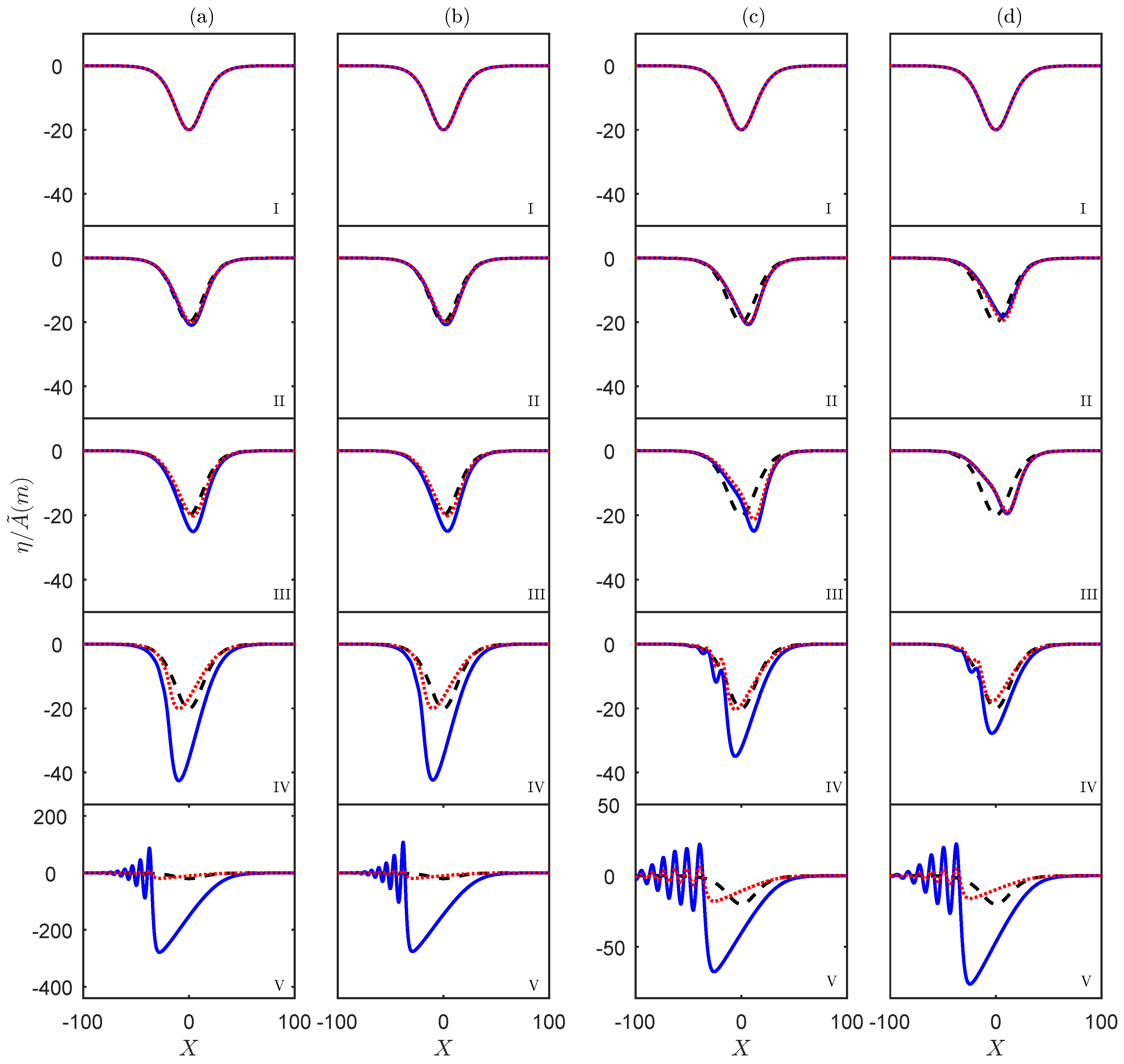
3.1.3. C: North West Shelf

We select a transect on the North West Shelf (NWS) of Australia from 114.5 E to 118.5 E, where the water depth ranges from 740 m to 120 m, which is shallower than that in the WP and SCS cases. This case is quite close to the location discussed by Grimshaw et al. [15] and Grimshaw et al. [16], and re-examined by Liu et al. [12] for the effect of the non-conservative term with coefficient $\sigma$. The main difference is that Grimshaw et al. [15] and Grimshaw et al. [16] used actual real oceanic data taken at the same time and location where the internal solitary waves were observed, whereas here we use monthly-mean climatological data, which can make some difference (see the discussion in the concluding Section 4). Figure 8 shows the background density and the corresponding buoyancy frequency for summer and winter. As the depth becomes shallower, there is a significant change in the pycnocline, and, as found by Grimshaw et al. [15] and Grimshaw et al. [16], there is a polarity change and the nonlinear coefficient $\mu$ changes sign from negative to positive. The vKdV coefficients are shown in Figure 9. Here, the background current $u_0$ ranges from −0.05 to 0.03 m s⁻¹ and has almost no effect on c, Q, $\mu$ and $\delta$, but does have some effects on $\beta$, of order ${10}^{-6}$ with the current and ${10}^{-8}$ without it.

From the simulation of the vKdV Equation (7) shown in Figure 10, we see that the initial internal solitary wave undergoes the well-known transformation due to the polarity change; an initial depression wave is converted to a depression rarefaction wave followed by an undular bore of elevation waves. From Figure 9, we see that $\beta$ has a significant effect during winter when the background current $u_0$ is taken into account, and is initially positive indicating wave decay, but then becomes negative and will generate some wave growth. In summer, the magnitude of $\beta$ is smaller and there is almost no big difference to the cases with or without the background current. Thus, the scaling factor R in winter has significant variation for the situation with a background current, varying from 1 to a minimum $0.8$, and then grows up to $1.3$; however, in summer there is no such difference. We note that the magnification factor Q changes from 1 to almost 0, and, when combined with R, generates a large difference between $\eta$ and $\tilde{A}$.

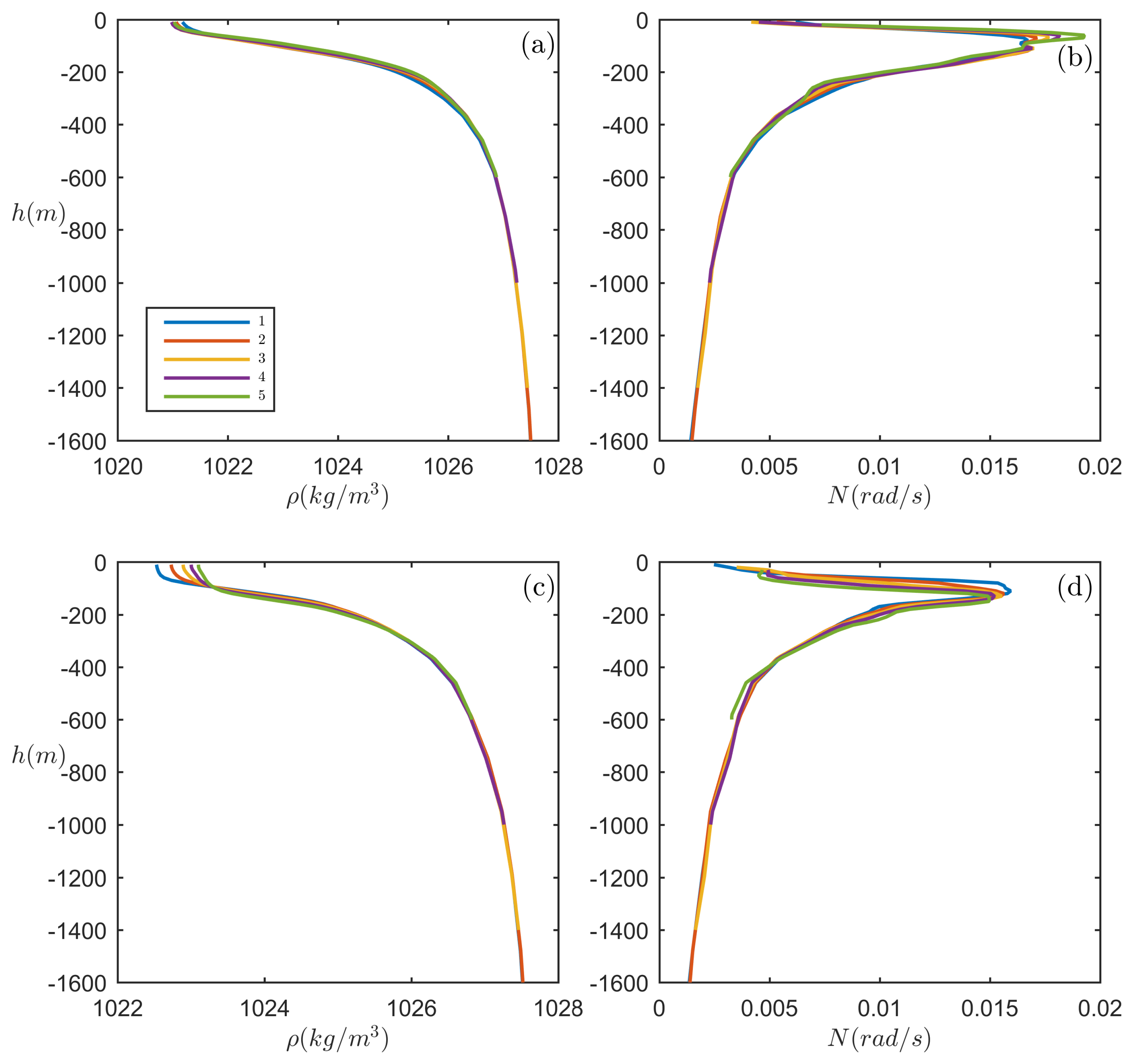
3.2. Cases Where the Horizontal Current Variation Is Significant

3.2.1. D: Malvinas Current

Internal waves propagating in the opposite direction along the very strong Malvinas Current (MC) in the southwest Atlantic Ocean have been observed (see Magalhaes and da Silva [17]). Our study region here is from shallow to deep along the transect 59.5 W which is near the shelf break and continental slope between 42.17 S and 43.5 S. Note that here the transect is in the N–S direction, so the x-direction is now also oriented N–S. The background state is shown in Figure 11 and the vKdV coefficients are shown in Figure 12. The water depth ranges from 200 m to 700 m. However, the depth of the background current data we can obtain is only from 100 m to 450 m, so we limit the depth to that range. The order of magnitude of the velocity of MC is 1 m s⁻¹ and can be almost up to 0.8 m s⁻¹ in the in situ observational data (Magalhaes and da Silva [17]), but here from the climatological data, the N–S velocity component of the current is only 0.1–0.25 m s⁻¹. However, nevertheless, this signal is much stronger than the above three cases. Compared to the long wave speed c, whose whole range is around 0.2–0.6 m s⁻¹ in Figure 12, we can see that it has the same magnitude as the background current. Thus, here, for the two scenarios with and without the background current, the difference of the original coefficients between these two situations is much clearer compared to those in the former cases, especially for the linear long wave phase speed c, the magnification factor Q, and the derived coefficient $\beta$.

This is an unusual case, as the internal solitary wave propagates from the shallow water to the deep water (see the depth h in Figure 12). In summer, the density and buoyancy frequency distribution in Figure 11 show that, along the transect, the pycnocline becomes thinner and shallower and this leads to a polarity change (see $\mu ,\alpha$ in Figure 12). The simulation of the vKdV Equation (7) is shown in Figure 13, and we see that an elevation wave is converted to a rarefaction elevation wave followed by an undular bore depression wave, with the coefficient $\mu$ of the quadratic nonlinear term being initially positive and then becomes negative. In winter, the background state distribution is similar to those in WP and SCS cases, with the pycnocline staying near the surface, and hence, there is just a depression wave with no polarity change.

A comparison of the cases when $\beta =0$ and $\beta \ne 0$ made by Liu et al. [12] suggests that the overall structure of the dynamical wave evolution remains basically the same, and the role of $\beta$ through R is usually mainly to change the wave amplitude. However, in this case, we can see significant influence on the shape as well as the amplitude. In Figure 13, we can see that the magnitude of the initial amplitude in each panel is 10 m, which is the same, and in the scenario with no background current, the wave decays in summer but grows slightly in winter. Although both of the wave variation trends in summer and winter correspond to those without the background current, when the background current is included, the wave shape is discernibly different. With much larger changes in R in this case, the derived nonlinear coefficient $\tilde{\alpha }$ is significantly modified compared to $\alpha$, which will then alter the nonlinear processes. Thus, here the effect of the current can cause stronger nonlinear phenomenon seen in Figure 13, compared to the weaker nonlinear effects when $u_0$ is not included.

3.2.2. E: Amazon River Mouth

A wave field of internal solitary waves extending more than 500 km near the Amazon River mouth (ARM) has been documented by Lentini et al. [18]. However, this region has not received much attention, even although the internal solitary waves here propagate over a large distance and are of frequent occurrence. Three distinct groups of waves were identified based on their sea surface signature and the main directions of propagation. While cross-shelf internal wave propagation has been previously documented, the majority of internal waves propagate along the shelf and upstream, approximately in the opposite direction from the North Brazilian Current (NBC) (see Lentini et al. [18]). For this case, the study area is along 48.5 W, from 3.83 N to 2.50 N, a transect of about 150 km distance. From Figure 14, we see that the background stratification is very similar to the SCS case, slowly changing density and an approximate two-layer stratification, with a near-surface pycnocline. In addition, here again, the transect is N–S. The vKdV coefficients are shown in Figure 15. The depth in this region is quite similar to that in the SCS case. The order of the alongshore currents that flow below the plume layer is 1 m s⁻¹, according to a series of current meter observation (see Johns et al. [19]). Here again, based on the climatological data, the current we use is weaker than that, with a range of 0.4–0.6 m s⁻¹ (N–S component) and 0.2–0.5 m s⁻¹ (W–E component). Although it is smaller than the in situ value, the background current is much stronger than that in the Malvinas Current case. Again, the current now makes an obvious difference to all the original coefficients (c, Q, $\mu$, $\delta$), not only on c and Q as in the previous cases. For the derived coefficient $\beta$, the order of magnitude is $O\left({10}^{-5}\right)$ compared to that without the current $O\left({10}^{-8}\right)$.

In this case, the vKdV simulations shown in Figure 16 show a seasonal difference as well as an effect of the background current. In Figure 15, we see that $\beta$ has significant differences between the cases with and without the consideration of the background current. It grows from 0 to positive when there is background current effect, and correspondingly the scaling factor R decays from 1 to $0.5$ ($0.4$) during winter (summer), indicating significant wave decay. In Figure 16, for example, the wave amplitude increases from initially 20 m to 40 m without the consideration of the background current in summer, but decreases to less than 10 m when the current is taken into account. There is a similar trend in winter. This case has similar depth and linear long wave speed c to the SCS case. However, the results are different. The background current along the transect in SCS is −0.15 to 0.15 m s⁻¹, much smaller than here. In terms of c, the magnitude of the background current contributes significantly. From Figure 16, we see that, although the initial wave amplitude is the same in these four panels, the wave evolution is clearly different in each, and both the wave structure and amplitude have been significantly modified due to the effects of the background current. The difference between the physical solution $\eta$ and the numerical solution $\tilde{A}$ is the joint influence of Q and R (see Formulas (2) and (7)), so, for the situation without the current, it mainly depends on Q, while, in the other scenario with a current, it mainly depends on R.

4. Discussion and Conclusions

In this paper, a sequel to Liu et al. [12], we have especially examined the effect of a background current on the non-conservative term $\sigma \eta$ in the vKdV Equation (1). This term, which has been neglected in most previous studies, was examined in Liu et al. [12], using actual oceanic data in three different cases considered by Grimshaw et al. [15]. Here, since background current data is not always readily available from in situ data, instead we use monthly mean climatological data along transects where large amplitude internal solitary waves have been observed. We choose five representative cases (A–E), representing five contrasting scenarios; from deep to shallow (A–D), with (C–D) or without (A, B and E) polarity changes and with different background current intensity (A–E). They are Western Portugal (WP), South China Sea (SCS), North West Shelf (NWS) of Australia, a region along the Malvinas Current (MC) and Amazon River mouth (ARM). In each case, we use monthly-mean climatological data, including variable background density and background currents, to calculate the coefficients of the vKdV Equation (1) for a mode 1 wave, and then simulate the propagation of an internal solitary wave propagation based on the vKdV Equation (5). In all cases, the derived nonlinear coefficient $\alpha$ is much larger than the derived non-conservative coefficient $\beta$, so that the effect of this non-conservative term is locally quite small. However, its effect is cumulative when expressed through the factor R, and in some cases this can be quite significant.

Both the horizontal density stratification and the background current contribute to the non-conservative term coefficient $\sigma$. In the cases A, B and C, where the horizontal density stratification is the major effect, the currents are small and the depth varies from deeper water in case A to shallower in case C. In a deep ocean, the background current is insignificant compared with the wave phase speed, and therefore makes very little difference on internal solitary waves, so the impact of the current can be neglected (see case A for instance). As the depth becomes shallower, such as in the cases B and C, with a relatively larger background current, the impact of the non-conservative term can have an effect on the waves, by making them grow or decay, or modifying the degree of the nonlinearity and dispersion. However, in cases D and E, the horizontal current variation is comparable to the background density stratification variation. In these two cases, there are two strong currents, the Malvinas Current and the North Brazilian Current, whose magnitudes can be 5–10 times greater than those in case A–C. Thus, in case D, where the depth is quite shallow together with a strong background current, we find a quite surprisingly large effect. Although the magnitude of the current in this case D is similar to the current in case B, the effect of the term $\sigma \eta$ is clearly different. The magnitude of the amplitude is clearly changed with stronger nonlinearity in case D, while there is not much difference in case B. The reason for this difference is because, with the larger depth, the linear long wave phase speed c is very different (see Figure 6 and Figure 12). The wave speed c in case D is much smaller, and so the background current is relatively larger, and so the term $\sigma \eta$ becomes more significant. When the background current is even larger still, as in case E, the wave amplitude can be totally different in both seasons. They reduce to less than 10 m from initially 20 m under the consideration of the current but grow when the current is not taken into account.

Furthermore, we note that only steady state currents are considered here as the data is time-averaged climatological data, and so the background flow is necessarily steady. In practice, time variation in the background flow, for instance in a tidal flow, could be significant (see Zhou and Grimshaw [11]). In addition, we note that, for the cases studied in this paper, all the speeds for internal waves are faster than the currents, so no blocking can occur, with turning points, which will lead to the internal waves amplifying and changing direction.

Our discussion has of necessity been based on the vKdV model (1) which strictly is valid only for weakly nonlinear waves, although is often used with some success for large amplitude waves (see Ostrovsky and Stepanyants [3], for instance). However, all the cases we have examined in this paper meet the KdV weak nonlinearity criterion. To demonstrate this, the plots of basic density stratification for each case (see that Figure 2, Figure 5, Figure 8, Figure 11 and Figure 14 show that the initial solitary amplitudes are smaller than the pycnocline depth). Nevertheless, the KdV equation and its variations are widely used, and work well with its well-known strengths and limitations. These KdV models describe the essential dynamics of observed internal solitary waves (and undular bores, not considered here) due to the underlying balance between nonlinearity and dispersion, even when the solutions may not be completely quantitatively correct.

Finally, we recall that we have used monthly-mean data for the background density stratification and currents, whereas observed internal waves in fact propagate on a particular instance of these background fields. Hence, the evolution might well be different from that found here. Out of necessity, we chose to use monthly averaged data instead of in situ data, as the background current in in situ data is rarely available in the form we needed. However, in order to test how large the difference might be, we increased and decreased the background current by 30% and then performed the same simulations for the wave propagation as that shown above. We then averaged the two maximum wave amplitudes obtained from these two contrived cases, and compared the outcome with the maximum amplitude we obtained from waves propagating on the mean background state. The results are shown in

Table 1. Wave amplitude comparison. S is summer, W is winter.

Case	A		B		C		D		E
Season	S	W	S	W	S	W	S	W	S	W
$(\overline{\eta }-\eta )/\eta (\%)$	$2.74$	$0.00$	$2.43$	$-1.80$	$2.06$	$2.52$	$-1.41$	$2.10$	$44.42$	$6.14$
$(\overline{\tilde{A}}-\tilde{A})/\tilde{A}(\%)$	$1.40$	$0.00$	$2.50$	$-0.60$	$0.00$	$0.16$	$0.70$	$1.35$	$2.73$	$-1.28$

with the comparison of the wave amplitudes between propagation on the mean ($\eta$, $\tilde{A}$) with the mean of the two contrived cases ($\overline{\eta }$, $\overline{\tilde{A}}$), both for the physical solutions ($\overline{\eta }$, $\eta$) and the numerical solutions ($\overline{\tilde{A}}$, $\tilde{A}$) of the transformed equation. From Table 1, we can see that indeed the propagation on the average background state is different from the averaged of the two inflated and deflated cases. However, for cases A–D, this difference is not significant, and we infer that the results presented in Section 3 are representative of the possible effects of background currents. However, for case E in summer, although the simulated evolution is comparable (plots not shown here), there is a significant difference in the maximum amplitude for the physical solution, although this is not so evident in the simulated solution. We suggest that the reason is that in this case E the current is quite strong, and we find that the change in the cumulative parameter R is quite significant, and so the averaged maximum amplitude $\overline{\eta }$ for the two scenarios is different from that when we use the monthly mean current.

References

1. Grimshaw, R. Internal solitary waves. In Environmental Stratified Flows; Grimshaw, R., Ed.; Kluwer: Boston, MA, USA, 2001; pp. 1–27. [Google Scholar]
2. Holloway, P.; Pelinovsky, E.; Talipova, T. Internal tide transformation and oceanic internal solitary waves. In Environmental Stratified Flows; Grimshaw, R., Ed.; Kluwer: Boston, MA, USA, 2001; pp. 31–60. [Google Scholar]
3. Ostrovsky, L.A.; Stepanyants, Y.A. Internal solitons in laboratory experiments: Comparison with theoretical models. Chaos 2005, 28, 037111. [Google Scholar] [CrossRef] [PubMed]
4. Helfrich, K.R.; Melville, W.K. Long nonlinear internal waves. Ann. Rev. Fluid Mech. 2006, 38, 395–425. [Google Scholar] [CrossRef]
5. Grimshaw, R. Internal solitary waves in a variable medium. Ges. Angew. Math. 2007, 30, 96–109. [Google Scholar] [CrossRef] [Green Version]
6. Grimshaw, R.; Pelinovsky, E.; Talipova, T.; Kurkina, A. Internal solitary waves: Propagation, deformation and disintegration. Nonlinear Process. Geophys. 2010, 17, 633–649. [Google Scholar] [CrossRef]
7. Vlasenko, V.I.; Stashchuk, N.M.; Hutter, K. Baroclinic Tides: Theoretical Modelling and Observational Evidence; Cambridge University Press: Cambridge, UK, 2005. [Google Scholar]
8. Benney, D.J. Long non-linear waves in fluid flows. J. Math. Phys. 1966, 45, 52–63. [Google Scholar] [CrossRef]
9. Benjamin, T.B. Internal waves of finite amplitude and permanent form. J. Fluid Mech. 1966, 25, 241–270. [Google Scholar] [CrossRef]
10. Grimshaw, R. Evolution equations for long nonlinear internal waves in stratified shear flows. Stud. Appl. Math. 1981, 65, 159–188. [Google Scholar] [CrossRef]
11. Zhou, X.; Grimshaw, R. The effect of variable currents on internal solitary waves. Dyn. Atmos. Oceans 1989, 14, 17–39. [Google Scholar] [CrossRef] [Green Version]
12. Liu, Z.; Grimshaw, R.; Johnson, E. Internal solitary waves propagating through variable background hydrology and currents. Ocean Model. 2017, 116, 134–145. [Google Scholar] [CrossRef]
13. Andrews, D.G.; McIntyre, M.E. On wave-action and its relatives. J. Fluid Mech. 1978, 89, 647–664. [Google Scholar] [CrossRef]
14. Grimshaw, R. Wave action and wave-mean flow interaction, with application to stratified shear flows. Ann. Rev. Fluid Mech. 1984, 16, 11–44. [Google Scholar] [CrossRef]
15. Grimshaw, R.; Pelinovsky, E.; Talipova, T.; Kurkin, A. Simulation of the transformation of internal solitary waves on oceanic shelves. J. Phys. Ocean 2004, 34, 2774–2779. [Google Scholar] [CrossRef]
16. Grimshaw, R.; Pelinovsky, E.; Stepanyants, Y.; Talipova, T. Modelling internal solitary waves on the Australian North West shelf. Mar. Freshw. Res. 2006, 57, 265. [Google Scholar] [CrossRef]
17. Magalhaes, J.M.; da Silva, J.C. Internal Waves Along the Malvinas Current: Evidence of Transcritical Generation in Satellite Imagery. Oceanography 2017, 30, 110–119. [Google Scholar] [CrossRef]
18. Lentini, C.A.; Magalhaes, J.M.; da Silva, J.C.; Lorenzzetti, J.A. Transcritical Flow and Generation of Internal Solitary Waves off the Amazon River: Synthetic Aperture Radar Observations and Interpretation. Oceanography 2016, 29, 187–195. [Google Scholar] [CrossRef] [Green Version]
19. Johns, W.E.; Lee, T.N.; Beardsley, R.C.; Candela, J.; Limeburner, R.; Castro, B. Annual Cycle and Variability of the North Brazil Current. J. Phys. Oceanogr. 1998, 28, 103–128. [Google Scholar] [CrossRef]
20. Ostrovsky, L. Nonlinear internal waves in a rotating ocean. Oceanology 1978, 18, 119–125. [Google Scholar]
21. Grimshaw, R. Evolution equations for weakly nonlinear, long internal waves in a rotating fluid. Stud. Appl. Math. 1985, 73, 1–33. [Google Scholar] [CrossRef]
22. Grimshaw, R.; Helfrich, K.R. Long-time solutions of the Ostrovsky equation. Stud. Appl. Math. 2008, 121, 71–88. [Google Scholar] [CrossRef]
23. Grimshaw, R.; da Silva, J.C.B.; Magalhaes, J.M. Modelling and observations of oceanic nonlinear internal wave packets affected by the Earth’s rotation. Ocean Model. 2017, 116, 146–158. [Google Scholar] [CrossRef]
24. Grimshaw, R. Models for nonlinear long internal waves in a rotating fluid. Fundam. Appl. Hydrophys. 2013, 6, 4–13. [Google Scholar]
25. Grimshaw, R.; Helfrich, K.; Johnson, E. The reduced Ostrovsky equation: Integrability and breaking. Stud. Appl. Math. 2012, 129, 414–436. [Google Scholar] [CrossRef]
26. Farmer, D.; Li, Q.; Park, J. Internal wave observations in the South China Sea: The role of rotation and non-linearity. Atmosphere-Ocean 2009, 47, 267–280. [Google Scholar] [CrossRef]
27. Li, Q.; Farmer, D.M. The generation and evolution of nonlinear internal waves in the deep basin of the South China Sea. J. Phys. Ocean. 2011, 41, 1345–1363. [Google Scholar] [CrossRef]
Figure 1. Five oceanic transects where internal solitary waves are known to occur frequently.
Fluids 03 00096 g001
Figure 2. Background density and buoyancy frequency distribution along the transect of the Western Portugal case. (a,b) are situations in summer, while (c,d) are in winter. Five different lines in each panel represent situations on the chosen five points along the wave propagation transect.
Fluids 03 00096 g002
Figure 3. Variation of the original coefficients (left panel and top of the right panel) and the derived coefficients (remainder of the right panel) of the vKdV equation for conditions of the Western Portugal case. The results show the coefficients in summer with background current u 0 (blue, solid), without u 0 (black, dash) and the coefficients in winter with u 0 (red, solid), without u 0 (blue, dashed-dotted).
Fluids 03 00096 g003
Figure 4. A numerical simulation of the vKdV Equation (5) for the Western Portugal case for summer (a,b) and winter (c,d) conditions, with u 0 = 0 (a,c) or u 0 0 (b,d), respectively. The initial condition is the solitary wave (black, dash), the numerical solution is A ˜ (red, dot) and the physical solution is η (blue, solid). From top to bottom, the distances from the initial point are (I) 0 km, (II) 110 km, (III) 220 km, (IV) 330 km, (V) 440 km, respectively.
Fluids 03 00096 g004
Figure 5. Background density and buoyancy frequency distribution along the transect of the South China Sea case. (a,b) are situations in summer, while (c,d) are in winter. Five different lines in each panel represent situations on the chosen five points along the wave propagation transect.
Fluids 03 00096 g005
Figure 6. Variation of the original coefficients (left panel and top of the right panel) and the derived coefficients (remainder of the right panel) of the vKdV equation for conditions of the South China Sea case. The results show the coefficients in summer with background current u 0 (blue, solid), without u 0 (black, dash) and the coefficients in winter with u 0 (red, solid), without u 0 (blue, dashed-dotted).
Fluids 03 00096 g006
Figure 7. A numerical simulation of the vKdV Equation (5) for the South China Sea case for summer (a,b) and winter (c,d) conditions, with u 0 = 0 (a,c) or u 0 0 (b,d), respectively. The initial condition is the solitary wave (black, dash), the numerical solution is A ˜ (red, dot) and the physical solution is η (blue, solid). From top to bottom, the distances from the initial point are (I) 0 km, (II) 110 km, (III) 220 km, (IV) 330 km, (V) 440 km, respectively.
Fluids 03 00096 g007
Figure 8. Background density and buoyancy frequency distribution along the transect of the North West Shelf case. (a,b) are situations in summer, while (c,d) are in winter. Five different lines in each panel represent situations on the chosen five points along the wave propagation transect.
Fluids 03 00096 g008
Figure 9. Variation of the original coefficients (left panel and top of the right panel) and the derived coefficients (remainder of the right panel) of the vKdV equation for conditions of the North West Shelf case. The results show the coefficients in summer with background current u 0 (blue, solid), without u 0 (black, dash) and the coefficients in winter with u 0 (red, solid), without u 0 (blue, dashed-dotted).
Fluids 03 00096 g009
Figure 10. A numerical simulation of the vKdV Equation (5) for the North West Shelf case for summer (a,b) and winter (c,d) conditions, with u 0 = 0 (a,c) or u 0 0 (b,d), respectively. The initial condition is the solitary wave (black, dash), the numerical solution is A ˜ (red, dot) and the physical solution is η (blue, solid). From top to bottom, the distances from the initial point are (I) 0 km, (II) 110 km, (III) 220 km, (IV) 330 km, (V) 440 km, respectively.
Fluids 03 00096 g010
Figure 11. Background density and buoyancy frequency distribution along the transect of the Malvinas Current case. (a,b) are situations in summer, while (c,d) are in winter. Five different lines in each panel represent situations on the chosen five points along the wave propagation transect.
Fluids 03 00096 g011
Figure 12. Variation of the original coefficients (left panel and top of the right panel) and the derived coefficients (remainder of the right panel) of the vKdV equation for conditions along the Malvinas Current case. The results show the coefficients in summer with background current u 0 (blue, solid), without u 0 (black, dash) and the coefficients in winter with u 0 (red, solid), without u 0 (blue, dashed-dotted).
Fluids 03 00096 g012
Figure 13. A numerical simulation of the vKdV Equation (5) of a transect along the Malvinas Current case in summer (a,b) and winter (c,d) conditions, with u 0 = 0 (a,c) or u 0 0 (b,d), respectively. The initial condition is the solitary wave (black, dash), the numerical solution is A ˜ (red, dot) and the physical solution is η (blue, solid). From top to bottom, the distances from the initial point are (I) 0 km, (II) 36.5 km, (III) 73 km, (IV) 109.5 km, (V) 146 km, respectively.
Fluids 03 00096 g013
Figure 14. Background density and buoyancy frequency distribution along the transect of the Amazon River Mouth case. (a,b) are situations in summer, while (c,d) are in winter. Five different lines in each panel represent situations on the chosen five points along the wave propagation transect.
Fluids 03 00096 g014
Figure 15. Variation of the original coefficients (left panel and top of the right panel) and derived coefficients (remainder of the right panel) of the vKdV equation for conditions of the Amazon River Mouth case. The results show the coefficients in summer with background current u 0 (blue, solid), without u 0 (black, dash) and the coefficients in winter with u 0 (red, solid), without u 0 (blue, dashed-dotted).
Fluids 03 00096 g015
Figure 16. A numerical simulation of the vKdV Equation (5) of a transect close to the Amazon River Mouth case in summer (a,b) and winter (c,d) conditions, with u 0 = 0 (a,c) or u 0 0 (b,d), respectively. The initial condition is the solitary wave (black, dash), the numerical solution is A ˜ (red, dot) and the physical solution is η (blue, solid). From top to bottom, the distances from the initial point are (I) 0 km, (II) 36.5 km, (III) 73 km, (IV) 109.5 km, (V) 146 km, respectively.
Fluids 03 00096 g016