Abstract
Multiple zonal jets observed in many parts of the global ocean are often embedded in large-scale eastward and westward vertically sheared background flows. Properties of the jets and ambient eddies, as well as their dynamic interactions, are found to be different between eastward and westward shears. However, the impact of these differences on overall eddy dynamics remains poorly understood and is the main subject of this study. The roles of eddy relative vorticity and buoyancy fluxes in the maintenance of oceanic zonal jets are studied in a two-layer quasigeostrophic model. Both eastward and westward uniform, zonal vertically sheared cases are considered in the study. It is shown that, despite the differences in eddy structure and local characteristics, the fundamental dynamics are essentially the same in both cases: the relative-vorticity fluxes force the jets in the entire fluid column, and the eddy-buoyancy fluxes transfer momentum from the top to the bottom layer, where it is balanced by bottom friction. It is also observed that the jets gain more energy via Reynolds stress work in the layer having a positive gradient in the background potential vorticity, and this is qualitatively explained by a simple reasoning based on Rossby wave group velocity.
1. Introduction
Jets are zonally elongated large-scale structures that are seen in the atmospheres of Jupiter and Saturn [1,2], as well as in the oceans [3,4,5,6,7]. Jets are formed in rapidly rotating systems in which mesoscale energetic eddies interact with Rossby waves. The argument in a barotropic model is that, in the presence of Rossby waves, the isotropic inverse cascade of kinetic energy stops near a meridional length scale set by Rossby waves resulting in the formation of zonal jets [8,9]. Jet formation can also be understood in terms of potential vorticity (PV) mixing by eddies. PV mixing produces a staircase structure in the PV distribution and, consequently, jets [10,11]. Although the two arguments approach the problem from different perspectives, they are perfectly consistent with each other. Numerous studies have confirmed the formation of jets in numerical models [4,12,13,14,15,16,17,18,19,20,21,22,23,24] (and others) as well as in laboratory experiments [25,26], which are generally in agreement with Rhines theory. However, in baroclinic models, jet formation can also be due to nonlocal energy transfer by interactions between barotropic and baroclinic modes [27,28] and the inverse cascade argument need not hold true. Reference [29] studied jet formation in a differentially heated rotating annulus experiment and found evidence of direct energy transfer to jets from eddies. Contrary to the upscale energy-transfer scenario, in some flow regimes jets can directly extract energy from the imposed background shear, rather than from the eddies (e.g., Reference [30]).
Here, we study the jet dynamics in the oceans using a baroclinic quasigeostrophic (QG) model. Idealized QG models have provided much understanding of jet dynamics. In a statistically steady state, multiple jets consist of sharper eastward jets and broader westward return flows. This feature is well-captured in stochastically forced, dissipative barotropic models [14,31,32,33] as well as in baroclinic models forced with a background vertical shear [16,27,28]. The meridional width of jets decreases with increasing the magnitude of the meridional gradient of planetary vorticity and increases with increasing the eddy energy, which is generally in agreement with Rhines scaling [8]. In addition, zonal jets act like partial barriers to meridional transport, and eddy diffusivity reduces across strong jets [34,35]. Cumulant expansion methods and the stochastic structural theory also predict the jet formation in the -plane barotropic turbulence [36,37,38,39].
The maintenance of jets is generally associated with the eddy relative-vorticity flux (convergence of eddy momentum flux), which is well-captured in QG models [16,18,27,40]. Eddies force the jets via Reynolds stresses, which are antifrictional for meridionally oriented eddies [34,41]. Indeed, the vertical flow structure is also important, and the significance of eddy-buoyancy effects has been pointed out in two-layer QG models [27,28,42,43]. It has been observed that zonal mean flow is not forced with the same intensity in both layers, and there is a strong disparity in the strength of the upper and lower layer Reynolds stresses, even though the flow is predominantly barotropic [27]. The role of eddy fluxes also depends on the direction of the imposed vertical shear (eastward/westward). References [28,42,43] studied the role of eddies in maintaining the jets, and found that the Reynolds stress and form stress forcing terms have the opposite effect on baroclinic jets in systems forced with an eastward vs a westward vertical shear. These observations play an important role in the dynamics, as they predict different barotropic–baroclinic interactions, yet a physical explanation of the directional asymmetry is still missing.
In this work, we study the eddy effects in a two-layer QG model, which we force with a uniform background flow in the upper layer. In general, atmospheric jet studies use an eastward background flow because the equator-to-pole temperature gradient results in an eastward vertical shear governed by thermal-wind balance. However, in the oceans, jets can experience either eastward or westward shear depending on the geographical location, e.g., jets seen in oceanic midlatitude gyre circulations. Thus, we consider both eastward and westward background vertical shear to assess the eddy impact on jets. Note that, unlike using barotropic–baroclinic (BT–BC) flow decomposition as in Reference [28,42], we deliberately performed analysis on individual layers. The primary reason for this choice is that the vertical eigenmodes are mixed barotropic–baroclinic modes because of the presence of the imposed vertical shear and bottom friction in the model [44,45]. This is an important aspect for the goal of this study because it is difficult to assess the role of eddies in terms of interacting barotropic and baroclinic modes, and interpreting the dynamics in terms of vertical modes can sometimes be misleading. We compare the role of eddies in the two cases and argue that on the fundamental level the dynamics are essentially the same in both cases, despite the reversal in the relative roles of the baroclinic Reynolds and form stresses.
The manuscript is organized into five sections. The model is described in Section 2, and the results are in Section 3. The results section has four subsections, in which we analyze the eddy stress terms, zonal energy balance, and the impact of bottom friction, and then compare the results with previous studies. A physical reasoning for the disparity in the strength of Reynolds stresses in individual layers is given in Section 4. Finally, the paper is concluded in Section 5.
2. Two-Layer QG Model
We use the two-layer QG model in this study. The model is forced with a uniform zonal background flow, , in the upper layer, and the bottom topography is flat [16,46]. The total depth is 4 km, where the top and bottom isopycnal layers are 1 km () and 3 km () deep, respectively. The governing equations are given as:
where is the Jacobian; () represents the top (bottom) layer; and is the Kronecker delta. Here, is the total PV in the layer, which is defined as:
Here, , and we use symbol to represent the PV of the developed flow. is the layerwise velocity stream function, and represents the meridional gradient of the Coriolis parameter ( is the angular velocity due to the Earth’s rotation at some reference latitude). is the stratification parameter, and and represent the eddy-viscosity and bottom-friction coefficients, respectively.
The main focus of this work is to analyze the jet dynamics and role of eddies in systems forced with an eastward or westward imposed shear. For an eastward shear (ES), we imposed a background flow of 6 cm · s, whereas cm · s was imposed to create a zonal westward shear (WS). The rest of the parameter values were kept the same, i.e., m · s, which corresponds to a reference latitude of ; m and m; m · s and s. The stratification parameters correspond to a baroclinic Rossby radius of 25 km, which is a typical value for the midlatitudinal ocean. The magnitudes of the background flow in ES and WS cases were chosen such that the imposed shear was more than the critical shear required for the system to be baroclinically unstable while maintaining the computational efficiency. Note that the bottom-friction parameter value used in this work is smaller than the typical value of 10 s used in ocean models. This choice results in strong and clear jets (see Reference [43] for details), in which eddy impacts are easier to assess.
Numerical Computations and Spin-Up
We used a doubly periodic rectangular domain having an area of km with a spatial resolution of 1024 × 512 grid points. In both ES and WS cases, the system was baroclinically unstable for the chosen parameters. Baroclinic instability was well-resolved in the model as grid spacing was roughly 3 km. For numerical simulations, we used finite-difference discretization with advanced numerical scheme ’CABARET’ [47]. The model was initialized from a perturbed state. The linear dispersion relation in the two-layer QG system predicts that the fastest-growing mode in the presence of a vertical shear constitutes of meridionally oriented phase lines, and this is clearly seen in the PV snapshots in Figure 1. This mode becomes further unstable, and the system then develops multiple jets (for more details, see Reference [42]). Kinetic energy (, where A is the area of the domain) time series is also shown in Figure 1, and it is clear that the system reaches a statistical energy equilibrium state in 6–7 years. We ran the simulations for 20 years and used the last 10 years of data (about 180 snapshots) for the computations of the eddy fluxes and eddy forcing, which are discussed in the next section.
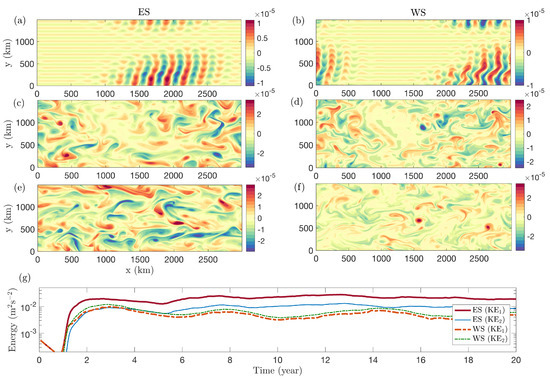
Figure 1.
(a–f) Snapshots of potential vorticity (PV) due to developed flow in the top layer at different times (top to bottom: snapshots at 400, 600, 1000 days) in eastward shear (ES) (left panels) and westward shear (WS) (right panels) cases and (g) kinetic energy time series (KE and KE in the legend represent the kinetic energy in the top and bottom layers, respectively).
Meridional profiles of the zonal velocity are shown in Figure 2. The profiles are averaged over the last 10 years of simulations and also zonally averaged. The alternating jet pattern is present in both ES and WS cases. There is one notable difference: in the case of a westward shear, jets are stronger in the bottom layer in comparison to the top layer, which is in contrast to the ES case (see also the kinetic energy time series in Figure 1). As a result of this, the barotropic and baroclinic flow components are of opposite phases in the WS case. Note also that the barotropic component of the mean flow is much stronger in comparison to the baroclinic component in both cases. These observations turned out to be important in understanding the eddy dynamics, and this is further discussed in the next section.
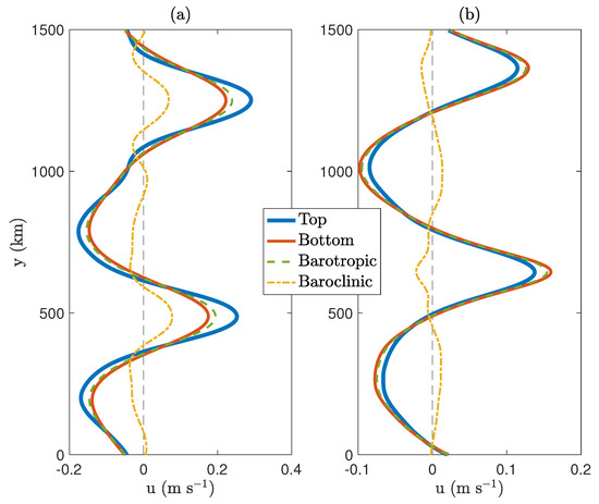
Figure 2.
Meridional profiles of the mean zonal velocity in the top and bottom layers (averaged in the zonal direction and time for the last 10 years)—(a) ES and (b) WS. Dashed and dash-dotted curves represent the barotropic () and baroclinic () components of the flow, respectively.
3. Role of Eddies
Eddies continuously interact with the large-scale mean flow, and play an important role in overall dynamics. In order to understand the eddy impact, we used Reynolds decomposition to separate the flow field into the zonally averaged time-mean flow (, where T and are the total time period for averaging and the zonal extent of the domain, respectively) and transient eddy field (). We used this decomposition in Equation (1) and then averaged in time as well as in the zonal direction. The resulting equations are given as:
where and are the velocity and relative vorticity, respectively. The overbar represents the mean in time and zonal direction. Note that and are the same as defined in Equations (1) and (2). The first two terms on the RHS represent the contribution from eddy relative vorticity and eddy buoyancy effects, respectively. These are the convergence of eddy relative vorticity and eddy buoyancy fluxes (eddy buoyancy fluxes are also known as heat fluxes) in each layer. We refer to these as Reynolds stress term (Rs) and form stress term (Fs) in the rest of the paper. Depending on the sign, stress terms can either create or remove the mean PV (in this paper, we use ‘mean PV’ to only refer to the PV of the developed mean flow). The sum of these two terms is generally referred to as ‘eddy forcing’ and, overall, the eddy-forcing term is responsible for maintaining the alternating jets. The rest of the terms on the RHS remove energy from the system through viscous dissipation and bottom drag. In the time mean, the time derivative of the mean PV vanishes and is kept only for clarity.
3.1. Reynolds and Form Stress Terms
In order to understand the role of eddies, we look at the impact of the Reynolds stress and form stress terms on the mean PV profile (see Equation (3)). Since the mean PV has a contribution from relative vorticity and buoyancy, it is better to separately investigate the effects of individual stress terms on mean relative vorticity and mean buoyancy. Here, we compare the meridional profiles of the mean relative vorticity and mean buoyancy (note that buoyancy contribution due to the imposed background flow is not included) with the meridional profiles of the Reynolds stress and form stress terms (Figure 3).
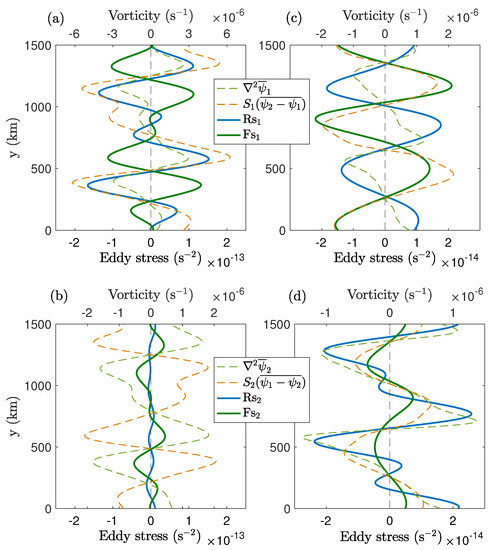
Figure 3.
Meridional profiles of the Reynolds stress (solid blue) and form stress (solid green) terms in the (a,c) top and (b,d) bottom layers. The (a,b) left and (c,d) right panels are for the ES and WS cases, respectively. The dashed curves represent the meridional profiles of the mean relative vorticity (dashed light green) and mean buoyancy (dashed orange) in the layers. The profiles are averaged in the zonal direction and time for the last 10 years. Additionally, the profiles of the stress terms are smoothened by applying moving averages in the meridional direction.
The first important aspect to notice is that, in both cases, the Reynolds stress term is positively correlated with the mean relative vorticity profile in both layers (see Table 1 for correlation coefficients). This shows that the Reynolds stress term forces the mean jets in the entire fluid column. This process of upgradient eddy-vorticity fluxes, which is responsible for persistent jets, is generally described as a negative viscosity effect [10,48]. Note that the strength of the Reynolds stress term differs in the individual layers because of the importance of the baroclinic effects [27]. In the ES case, the Reynolds stress term is more than five times stronger in the top layer than in the bottom layer. Similarly, in the WS case, the Reynolds stress term is stronger in the bottom layer. The layer with a stronger Reynolds stress term tends to be the more energetic layer. We discuss this aspect in more detail later in this paper.

Table 1.
Correlation coefficients of the meridional profiles of the mean vorticity and buoyancy with the meridional profiles of the Reynolds stress and form stress terms. i indicates the layer, and .
On the other hand, the form stress term seems to have opposite effects in the ES and WS cases, as the form stress term is negatively (positively) correlated with the mean buoyancy profile in the ES and WS cases (Table 1), respectively. However, we argue that eddies perform the same task in both cases. Bottom friction is the only large-scale energy sink in the model, which acts on the bottom layer. In both cases, the form stress term transfers momentum from the top to the bottom layer, which is then balanced by the bottom-friction term. Given the top layer is more energetic in the ES case, the eddy momentum transfer from the top to the bottom layer tends to reduce the mean shear () in the system. Hence, the form stress term acts opposite to the mean buoyancy in the system. In contrast, in the WS case, momentum transfer tends to make the bottom layer more energetic in comparison to the top layer, and the form stress term tends to enhance the magnitude of the mean buoyancy. This is similar to the case of Earth’s atmosphere, where baroclinic eddies transfer momentum from the middle atmosphere to the surface, which is then balanced by surface friction and the surface westerlies are produced [49].
We could also look at the effects of the form stress term on the mean relative vorticity profile or Reynolds stress term on the mean buoyancy profile. These effects would not be independent from what has been described above. For example, the form stress term transfers momentum from the top to the bottom layer; thus, it reduces the strength of the mean flow in the top layer and enhances the mean flow strength in the bottom layer. This is clearly seen in Figure 3 as the form stress term is negatively (positively) correlated with the mean relative vorticity profile in the top (bottom) layer. Similarly, to be consistent with the argument, the Reynolds stress term must be positively (negatively) correlated with the mean buoyancy in the more (less) energetic layer. In an overall balance, stress terms are such that eddies drive the jets. In both the ES and WS cases, the Reynolds stress term forces the jets in both layers, whereas the form stress term transfers momentum from the top to the bottom layer, where it is balanced by bottom friction. In essence, our layerwise analyses show that overall dynamics are essentially the same in both the ES and WS cases.
3.2. Zonal Energy Balance
It is interesting to note that the Reynolds stress term is stronger in the top layer in the ES case and in the bottom layer in the WS case, which are the more energetic layers in both cases. Reference [27] used a baroclinic QG model forced with an eastward shear and showed that the mean zonal flow receives almost all of the energy via the upper-layer Reynolds stresses. In order to analyze the energy exchange between the jets and eddies in individual layers, we derived the time-mean zonal energy balance by multiplying to Equation (1) in each layer and further averaging in space (denoted by ) and time [27]:
where and are the same as defined in Equations (1) and (2). The two terms on the RHS represent the energy exchange between the mean flow and eddy components in individual layers. In the first term, the zonal mean flow gains energy due to nonzero Reynolds stress correlations (RSC), which is basically the transfer of kinetic energy from eddies to the mean zonal flow. The top and bottom layers continuously interact and exchange energy through eddy-buoyancy effects, which is represented with the second term on the RHS (referred to as ‘form stress correlations’, FSC, from here onward) in Equation (4). The rest of the terms on the RHS represent the loss of the mean zonal energy through eddy viscosity and bottom friction. For completeness, we derived a single energy balance equation by multiplying the above equation by and adding them, which is given as:
In a statistical equilibrium, the total energy of the system is conserved, and the terms on the RHS in Equation (5) exactly balance each other (see Table 2). The mean zonal flow gains energy through RSC terms in both layers and most of the energy is dissipated through bottom friction. In both cases, FSC terms remove energy from the top layer and transfer energy into the bottom layer. This is in agreement with our hypothesis that, in both cases, eddies transfer momentum from the top to the bottom layer, where it is balanced by bottom friction.
Table 2.
Energy transfer via RSC and FSC terms, and dissipation terms (averaged in space and time for the last 10 years) in the top and bottom layers. The units are in 10 ms. is the Kronecker delta, and .
We also look at the meridional profiles of RSC, FSC, and dissipation terms in Equation (4), shown in Figure 4. The profiles show strong variability in the meridional direction, which is strongly correlated with the mean flow profile. For example, RSC terms are at the maximum in the region of eastward jets. In the regions of eastward jets, FSC terms remove energy from the mean zonal flow in the more energetic layer and force the mean zonal flow in the less energetic layer in both cases; however, in the process, the westward mean flow strengthens (weakens) in the more (less) energetic layer (compare the profiles of FSC terms in top and bottom panels in Figure 4). Although the effects of FSC terms on eastward and westward jets reverse in the individual layers in ES and WS cases, overall energy transfer via FSC terms is still from the top to bottom layer in both cases (Table 2). This energy is dissipated through bottom friction in the lower layer. Thus, the overall impact of eddy-buoyancy fluxes is to transfer energy to the surface where it is dissipated through bottom friction.
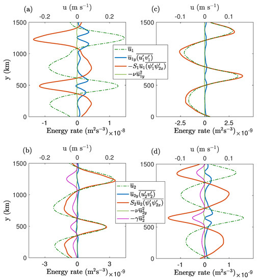
Figure 4.
Meridional profiles of Reynolds stress correlations (RSC), form stress correlations (FSC), and dissipation terms in both layers—(a,b) ES; (c,d) WS. and represent the meridional and zonal gradient of the mean zonal velocity and bottom layer stremfunction, respectively. Top and bottom panels correspond to the upper and lower layers. The mean flow in the layer is represented by dash-dotted curve. The profiles are averaged in the zonal direction and time for the last 10 years.
In general, eddy-buoyancy fluxes are downgradient as eddies work to flatten the isopycnals. In our study, buoyancy fluxes also tend to reduce to vertical velocity shear, as FSC terms force (act against) the eastward mean flow in the less (more) energetic layer (Figure 4). In order to confirm this, we computed heat diffusivity using the following relation:
Note that heat diffusivity can be computed using eddy velocity in either layer, but would result in the same profile. The meridional profiles of heat diffusivity are shown in Figure 5. In both cases, the heat-diffusivity coefficient is positive and of the same order of magnitude. Thus, the eddy-buoyancy fluxes are downgradient. On the other hand, the locations of the heat-diffusivity maxima relative to the jets are different in the two cases. In the ES case, heat diffusivity is strongest near the flanks of eastward jets whereas, in the WS case, the maxima in the heat-diffusivity profile coincide with the westward jets. In terms of eddy-buoyancy transport, both eastward and westward shear cases are similar as eddies tend to flatten the isopycnals, although the locations of the maxima in the heat-diffusivity profiles are different.
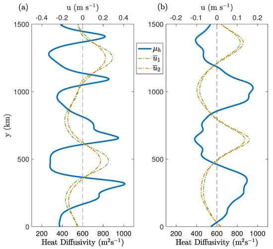
Figure 5.
Meridional profiles of heat diffusivity—(a) ES and (b) WS. Profiles were computed using the eddy-buoyancy fluxes that were averaged in the zonal direction and time for the last 10 years. The dash-dotted curves represent the meridional profiles of the mean flow in the layers. A positive value of heat diffusivity indicates that the eddy-buoyancy fluxes are downgradient.
3.3. Effect of Bottom Friction
The role of friction is crucial in governing ocean dynamics and the strength of large-scale currents in the oceans [50,51]. Reference [43] showed that the strength of bottom friction controls the multiple jets and their ambient eddies. Here, we probe into the effects of bottom friction on the baroclinic structure of the flow (see Equation (3) for the bottom layer). It can be inferred from Figure 3 that bottom friction has the opposite effect on the baroclinic structure in the ES and WS cases, as the meridional profiles of bottom-friction term and baroclinic stream function , are positively (negatively) correlated in the ES (WS) case. Hence, bottom friction tends to make the flow more baroclinic in the ES case, whereas bottom friction favors the barotropic structure in the flow in the WS case.
In order to understand this, we look at the mean zonal velocity profiles (Figure 2). The zonal mean flow is stronger in the top (bottom) layer in the ES (WS) case as the top (bottom) layer receives more energy through RSC terms. Most of the energy is dissipated through bottom friction (Table 2), which only acts on the lower layer. Thus, bottom friction removes energy primarily from the mean flow in the lower layer and, as a result of this, the flow structure tends to be more baroclinic and barotropic in the ES and WS cases, respectively. Although the dynamics are the same in the ES and WS cases, the response of the baroclinic structure changes entirely due to bottom friction.
3.4. Comparison with Previous Studies
In our layerwise analyses, we found that the role of eddies is the same in both the ES and WS case. In contrast, some previous works have found different results. For example, References [28,42] studied eddy dynamics in the presence of jets and found that the roles of Reynolds stress and form stress terms are opposite in systems forced with eastward and westward vertical shears. In the former, the Reynolds (form) stress term maintains (acts against) the baroclinic jets. On the other hand, the roles of the Reynolds stress and form stress terms reverse in the latter. Although the eddy dynamics in BT–BC analyses look significantly different in the two scenarios, we argue that eddies still behave the same way, as seen in our layerwise analyses.
To understand this, we look at the baroclinic flow structure in ES and WS cases (Figure 2). The barotropic and baroclinic flow are in phase in the ES case. On the other hand, they are of opposite phase in the WS case, and this is because the bottom layer is more energetic, which results in a baroclinic mean flow () that is of the opposite phase of the barotropic mean flow (). This reversal in the phase of the baroclinic mode is the key reason why the roles of the form stress and Reynolds stress terms look opposite in the two cases when interpreted in terms of barotropic and baroclinic modes. We observed the same in our results as the form stress term was negatively (positively) correlated with the mean buoyancy in the ES (WS) case (Figure 3), even though eddies transfer momentum from the top to the bottom layer in both cases. The same effect leads to a reversal in the effects of bottom friction on the baroclinic flow structure, which was discussed in the previous subsection. BT–BC decomposition is still helpful; however, additional attention should be paid while interpreting the dynamics in terms of modes. One way to avoid this ambiguity could be to define the baroclinic mode on the basis of the energy of the mean zonal flow in the layers, e.g., and in the ES and WS cases, respectively. This would ensure that barotropic and baroclinic modes are always in phase.
We would like to emphasize here that the goal of this work was only to analyze the overall role of eddies in the dynamics. Indeed, local eddy shapes and their meridional structure are different in eastward and westward shears (e.g., see the discussion in References [44,45]). In our results, the locations of the maxima in the meridional profiles of heat diffusivity in the ES and WS cases were also different. Studying the characteristics of eddy shapes is another interesting topic; however, this is beyond the scope of this work.
4. Disparity in the Upper- and Lower-Layer Reynolds Stress Correlations
We observed that, in both the ES and WS cases, the zonal mean flow preferred to receive more energy through RSC terms in one of the layers (Table 2). The meridional profiles of the RSC terms are shown in Figure 6. In agreement with Reference [27], the energy transfer through RSC term in the upper layer dominates in the ES case. On the other hand, the lower layer receives more energy via Reynolds stresses in the WS case. Thus, the layer receiving more energy through the RCS term tends to be more energetic (see Figure 2). Despite strong disparity in the strength of the RSC terms in the top and bottom layers, the flow is predominantly barotropic (Figure 2). This shows that the baroclinic structure plays an equally important role in jet dynamics as there is significant energy exchange between the layers (Table 2), and this effect may not be captured in a barotropic model.
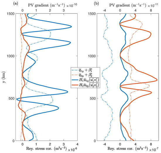
Figure 6.
Meridional profiles of energy transfer to the zonal mean flow through Reynolds stress correlations (solid) and meridional profiles of the meridional gradient in total PV (dash-dotted) in both layers—(a) ES; (b) WS. and represent the meridional gradient of the mean zonal velocity and mean PV, respectively; and () is the background PV gradient in ith layer. The profiles were averaged in the zonal direction and time for the last 10 years. The zonal mean flow receives more energy through Reynolds stress correlation in the upper (lower) layer in the ES (WS) case.
Given that both layers in the two-layer QG model experience the same magnitudes of velocity shear and stratification, the strong disparity in the strength of RSC terms is not obvious. Also, it is counterintuitive to see that the bottom layer is more energetic in the WS case, even though the westward background flow was imposed in the top layer. This indicates that the direction of the vertical shear is important rather than the layer in which the background flow is imposed. For example, one could also force the system with an eastward background flow in the lower layer, which would then create a westward shear in the vertical, and still the lower layer would be more energetic. We observed that, in both cases, the layer that was characterized by a positive background PV gradient received more energy through RSC terms (Figure 6). We also verified that the magnitude of the background PV gradient does not play any role here. We ran additional simulations with westward shear, where we imposed background flows of and cm · s in the upper layer, respectively. This resulted in a larger magnitude of the background PV gradient in the lower (upper) layer in cm · s ( cm · s) case. In all three simulations ( cm · s), we found that the lower layer was more energetic.
In order to understand this disparity in the upper- and lower-layer RSC terms, we analyze the eddy momentum fluxes more carefully. In general, a zonal mean flow can be generated by stirring due to baroclinic eddies. This stirring generates Rossby waves that carry energy away from the stirring region and eventually fade away or break and dissipate. Consequently, there is a strong convergence of eddy momentum into the stirring region. This results in an eastward zonal flow in the stirring region, and westward return flow in the wave-breaking region [52,53,54]. We can apply the same argument to the problem of multiple jets. As can be inferred from Figure 6, there is a strong convergence of eddy momentum into eastward jets in both layers. This indicates that, on average, Rossby waves carry energy from the regions of eastward jets to the westward jet regions. The direction of energy propagation is determined by the direction of group velocity, which we analyze in the linearized two-layer QG model. For simplicity, we treat the layers independent of each other by neglecting the buoyancy term perturbations in PV and also neglect the presence of jets. Then, approximate expressions for the dispersion relation and group velocity are given as (for a brief review, see Section 15.1.2 in Reference [55]):
where and are the frequency and meridional group velocity of Rossby waves in ith layer; is the background PV gradient; and k, l are the zonal and meridional wavenumbers, respectively ( is the Kronecker delta and ). Indeed, in the presence of multiple jets, Rossby wave dynamics is more complex than simple plane waves. Our aim here is only to understand the qualitative differences between the dynamics in terms of group velocity to examine why RSC terms differ in strength in the top and bottom layers. Since Reynolds stresses only depend on the eddy field, the presence of jets makes little difference. Reynolds stresses are also independent of the coupling between the layers. Hence, the usage of the simplified expressions is reasonable for our purposes.
Rossby waves carry energy away from the region of stirring, i.e., eastward jet cores (EJC). The direction of energy propagation is along the group velocity; thus, group velocity must be directed away from the stirring region [53]. In response, there is a convergence or divergence of momentum in EJC. For a disturbance of the form in the ith layer, the associated momentum flux is given as:
The direction of momentum flux depends on the sign of in each layer, which can be determined from Equation (8). is positive (negative) in the top (bottom) layer in the ES case, whereas it is positive (negative) in the bottom (top) layer in the WS case. For positive , northward (southward) of EJC we have (), which results in a convergence of eddy momentum into the eastward jets because this results in, northward of EJC and southward of EJC. Hence, eddies give energy to the eastward jets and make them sharper. On the other hand, for negative , northward (southward) of EJC, (), which results in a divergence of eddy momentum from the eastward jets and eddies tend to smoothen the jets. Thus, the jets are forced by eddies only for a positive background PV gradient. This simplified analysis predicts that Reynolds stresses should be more efficient in the top (bottom) layer in the ES (WS) case, which is clearly seen in Figure 6. Note that Reynolds stresses may still force the mean zonal flow in both layers as the dynamics in the two-layer QG model is more complex. However, we believe that the opposite signs of the background PV gradients in the layers would still affect the strength of Reynolds stresses.
Indeed, Equations (7) and (8) are a simplification, and group velocity would also depend on the mean flow and coupling between the layers. Our assumption of more stirring by eddies in eastward jet regions is only based on Figure 6, and we do not have any physical reasoning for this. However, our focus was only to understand the behavior of eddy momentum fluxes on the basis of the group-velocity direction, which we inferred from the fully nonlinear simulations (Figure 6). It is reasonable to believe that the group-velocity direction would be the same as deduced from Equation (8). Our crude analysis provides us with a reasonable explanation of why there should be disparity in the strength of Reynolds stresses. Although we only considered the background PV gradients in the layers, the argument also holds for the total layerwise PV gradients because the PV gradients are not significantly modified by the contribution from the developed flow (Figure 6). The more energetic layer is the one that experiences a positive meridional gradient in the background PV. Our qualitative analysis only explains the disparity in RSC terms in the top and bottom layers and does not predict their relative strengths. It also cannot predict which wave numbers contribute the most to eddy momentum convergence. Rigorous analysis that includes the presence of jets and buoyancy terms is necessary to address these aspects, which will be addressed in the future.
5. Summary
Multiple jets embedded in midlatitude gyre circulations and the southern oceans are seen in models and satellite observations. The jets are found in both eastward and westward sheared large-scale flows. In this study, we used an idealized two-layer QG setup forced with a uniform zonal vertical shear. The main aim was to understand how different or similar the dynamics in two systems are, in which one was forced with an eastward shear while the other was forced with a westward shear. We found that both systems were largely the same in terms of dynamics with a few differences. In both cases, eddies perform the same task, i.e., Reynolds stress terms force the jets in the entire fluid column, and the form stress term transfers momentum from the top layer to the bottom layer. We also confirmed this by analyzing the zonal mean energy balance. We found that, in an overall balance, eddies force the mean zonal flow via Reynolds stress correlations and transfer energy to the bottom layer via form stress correlations The momentum exchange between the top and bottom layers is in response to dissipation through bottom friction in the lower layer. As a result of this, the form stress term acts against the jets in the upper layer and forces the jets into the lower layer. The mechanism is similar to the dynamics in Earth’s atmosphere where eddies transfer momentum from the middle atmosphere to the surface, where it is balanced by surface friction [49].
At first glance, our results look somewhat in contrast to the studies by References [28,42], who concluded that dynamics are different in eastward- vs. westward-sheared flows. They found that the effects of the Reynolds stress and form stress terms on baroclinic jets are opposite in systems forced with an eastward vs. a westward vertical shear. However, deeper analysis revealed that the discrepancy between our results and previous works is due to the phase reversal of the mean baroclinic flow in the westward-sheared case. In the WS case, the bottom layer was more energetic, which resulted in a baroclinic flow that was in the opposite phase of the barotropic flow (Figure 2). Due to this reversal, the eddy effects look opposite, even though the overall dynamics are the same. For example, we found that bottom friction supports a baroclinic (barotropic) flow structure in the eastward (westward)-sheared case; however, both outcomes are just a result of momentum transfer by eddies from the top to the bottom layer and there is no difference in eddy dynamics in the two cases. Thus, the results presented in this study are consistent with References [28,42]. We would like to stress here that the goal of this work was only to study the overall behavior of eddies, which we found to be the same in both cases. Characteristics of meridional structure and eddy shapes are different in eastward- and westward-sheared cases [44,45].
Another important observation we made was that the mean zonal flow receives more energy through Reynolds stress correlations in one preferred layer (Table 2), which has been shown earlier [27]. We found that the disparity depends on the sign of the background PV meridional gradient, and the layer that experiences a positive gradient in the background PV receives more energy. In general, the maintenance of eastward jet cores can be understood in terms of stirring by baroclinic eddies, in which Rossby waves carry energy away from the stirring region, resulting in the convergence of eddy momentum into eastward jets [52,53,54]. We derived simplified expressions for the meridional group velocity of Rossby waves in both layers. We used the expressions to predict the direction of phase vectors associated with the group velocity of disturbances that propagate away from the region of stirring. For the phase vectors, we analyzed the direction of eddy momentum flux and found that there is a convergence of eddy momentum flux into eastward jets only in the layer having a positive meridional gradient in the background PV. This somewhat explains why Reynolds stresses are more efficient in either of the layers and are also in agreement with our simulations (Figure 6). We would like to stress here that the group-velocity expressions derived in this work are a simplification of the governing equations as we treated the layers independent of each other and neglected the presence of the jets. Nevertheless, our analysis provides us with a qualitative explanation for the discrepancy in the strength of Reynolds stresses. The usage of the expressions is limited to this work and extra care should be taken if a similar expression is used in other scenarios. A detailed computation that includes the contribution from the mean flow and coupling between the layers is required to quantitatively understand the efficiency of Reynolds stresses in each layer.
Author Contributions
H.K. performed the numerical experiments. H.K. and P.B. interpreted the results and wrote the paper.
Funding
This research received no external funding.
Acknowledgments
H.K. would like to acknowledge the support from President’s PhD scholarship and Mathematics for Planet Earth CDT at Imperial College. P.B. is funded by the NERC grant NE/R011567/1. The authors are grateful to the two anonymous reviewers for their comments and suggestions that improved the article. The authors would also like to thank the HPC team at Imperial College and Andrew Thomas for their help with computer clusters.
Conflicts of Interest
The authors declare no conflict of interest.
Abbreviations
The following abbreviations are used in this manuscript:
| PV | Potential vorticity |
| QG | Quasigeostrophic |
| BT-BC | Barotropic–Baroclinic |
| ES | Eastward shear |
| WS | Westward shear |
| Rs | Reynolds stress term |
| Fs | Form stress term |
| RSC | Reynolds stress correlations |
| FSC | Form stress correlations |
| EJC | Eastward jet cores |
References
- Ingersoll, A.P.; Beebe, R.F.; Mitchell, J.L.; Garneau, G.W.; Yagi, G.M.; Müller, J.P. Interaction of eddies and mean zonal flow on Jupiter as inferred from Voyager 1 and 2 images. J. Geophys. Res. Space Phys. 1981, 86, 8733–8743. [Google Scholar] [CrossRef]
- Gierasch, P.J.; Ingersoll, A.P.; Banfield, D.; Ewald, S.P.; Helfenstein, P.; Simon-Miller, A.; Vasavada, A.; Breneman, H.H.; Senske, D.A.; Team, G.I. Observation of moist convection in Jupiter’s atmosphere. Nature 2000, 403, 628–630. [Google Scholar] [CrossRef] [PubMed]
- Maximenko, N.A.; Bang, B.; Sasaki, H. Observational evidence of alternating zonal jets in the world ocean. Geophys. Res. Lett. 2005, 32, L12607. [Google Scholar] [CrossRef]
- Richards, K.J.; Maximenko, N.A.; Bryan, F.O.; Sasaki, H. Zonal jets in the Pacific Ocean. Geophys. Res. Lett. 2006, 33, L03605. [Google Scholar] [CrossRef]
- Sokolov, S.; Rintoul, S.R. Multiple jets of the Antarctic Circumpolar Current south of Australia. J. Phys. Oceanogr. 2007, 37, 1394–1412. [Google Scholar] [CrossRef]
- Ivanov, L.; Collins, C.; Margolina, T. System of quasi-zonal jets off California revealed from satellite altimetry. Geophys. Res. Lett. 2009, 36. [Google Scholar] [CrossRef]
- Van Sebille, E.; Kamenkovich, I.; Willis, J.K. Quasi-zonal jets in 3-D Argo data of the northeast Atlantic. Geophys. Res. Lett. 2011, 38, L02606. [Google Scholar] [CrossRef]
- Rhines, P.B. Waves and turbulence on a beta-plane. J. Fluid Mech. 1975, 69, 417–443. [Google Scholar] [CrossRef]
- Rhines, P.B. Jets. Chaos Interdiscip. J. Nonlinear Sci. 1994, 4, 313–339. [Google Scholar] [CrossRef] [PubMed]
- Dritschel, D.G.; McIntyre, M.E. Multiple jets as PV staircases: The Phillips effect and the resilience of eddy-transport barriers. J. Atmos. Sci. 2008, 65, 855–874. [Google Scholar] [CrossRef]
- Dunkerton, T.J.; Scott, R.K. A barotropic model of the angular momentum–conserving potential vorticity staircase in spherical geometry. J. Atmos. Sci. 2008, 65, 1105–1136. [Google Scholar] [CrossRef]
- Williams, G.P. Planetary circulations: 1. Barotropic representation of Jovian and terrestrial turbulence. J. Atmos. Sci. 1978, 35, 1399–1426. [Google Scholar] [CrossRef]
- Williams, G.P. Planetary circulations: 2. The Jovian quasi-geostrophic regime. J. Atmos. Sci. 1979, 36, 932–969. [Google Scholar] [CrossRef]
- Maltrud, M.E.; Vallis, G.K. Energy spectra and coherent structures in forced two-dimensional and beta-plane turbulence. J. Fluid Mech. 1991, 228, 321–342. [Google Scholar] [CrossRef]
- Vallis, G.K.; Maltrud, M.E. Generation of mean flows and jets on a beta plane and over topography. J. Phys. Oceanogr. 1993, 23, 1346–1362. [Google Scholar] [CrossRef]
- Panetta, R.L. Zonal jets in wide baroclinically unstable regions: Persistence and scale selection. J. Atmos. Sci. 1993, 50, 2073–2106. [Google Scholar] [CrossRef]
- Tréguier, A.M.; Panetta, R.L. Multiple zonal jets in a quasigeostrophic model of the Antarctic Circumpolar Current. J. Phys. Oceanogr. 1994, 24, 2263–2277. [Google Scholar] [CrossRef]
- Huang, H.P.; Robinson, W.A. Two-dimensional turbulence and persistent zonal jets in a global barotropic model. J. Atmos. Sci. 1998, 55, 611–632. [Google Scholar] [CrossRef]
- Berloff, P. On rectification of randomly forced flows. J. Mar. Res. 2005, 63, 497–527. [Google Scholar] [CrossRef]
- Lee, S. Baroclinic multiple zonal jets on the sphere. J. Atmos. Sci. 2005, 62, 2484–2498. [Google Scholar] [CrossRef]
- Nakano, H.; Hasumi, H. A series of zonal jets embedded in the broad zonal flows in the Pacific obtained in eddy-permitting ocean general circulation models. J. Phys. Oceanogr. 2005, 35, 474–488. [Google Scholar] [CrossRef]
- Nadiga, B.T. On zonal jets in oceans. Geophys. Res. Lett. 2006, 33, L10601. [Google Scholar] [CrossRef]
- Scott, R.K.; Polvani, L.M. Forced-dissipative shallow-water turbulence on the sphere and the atmospheric circulation of the giant planets. J. Atmos. Sci. 2007, 64, 3158–3176. [Google Scholar] [CrossRef]
- Kamenkovich, I.; Berloff, P.; Pedlosky, J. Role of eddy forcing in the dynamics of multiple zonal jets in a model of the North Atlantic. J. Phys. Oceanogr. 2009, 39, 1361–1379. [Google Scholar] [CrossRef]
- Read, P.; Yamazaki, Y.; Lewis, S.; Williams, P.D.; Miki-Yamazaki, K.; Sommeria, J.; Didelle, H.; Fincham, A. Jupiter’s and Saturn’s convectively driven banded jets in the laboratory. Geophys. Res. Lett. 2004, 31. [Google Scholar] [CrossRef]
- Read, P.L.; Yamazaki, Y.H.; Lewis, S.R.; Williams, P.D.; Wordsworth, R.; Miki-Yamazaki, K.; Sommeria, J.; Didelle, H. Dynamics of convectively driven banded jets in the laboratory. J. Atmos. Sci. 2007, 64, 4031–4052. [Google Scholar] [CrossRef]
- Thompson, A.F.; Young, W.R. Two-layer baroclinic eddy heat fluxes: Zonal flows and energy balance. J. Atmos. Sci. 2007, 64, 3214–3231. [Google Scholar] [CrossRef]
- Berloff, P.; Kamenkovich, I.; Pedlosky, J. A model of multiple zonal jets in the oceans: Dynamical and kinematical analysis. J. Phys. Oceanogr. 2009, 39, 2711–2734. [Google Scholar] [CrossRef]
- Wordsworth, R.; Read, P.; Yamazaki, Y. Turbulence, waves, and jets in a differentially heated rotating annulus experiment. Phys. Fluids 2008, 20, 126602. [Google Scholar] [CrossRef]
- Khatri, H.; Berloff, P. A mechanism for jet drift over topography. J. Fluid Mech. 2018, 845, 392–416. [Google Scholar] [CrossRef]
- Danilov, S.; Gryanik, V.M. Barotropic beta-plane turbulence in a regime with strong zonal jets revisited. J. Atmos. Sci. 2004, 61, 2283–2295. [Google Scholar] [CrossRef]
- Danilov, S.; Gurarie, D. Scaling, spectra and zonal jets in beta-plane turbulence. Phys. Fluids 2004, 16, 2592–2603. [Google Scholar] [CrossRef]
- Suhas, D.; Sukhatme, J. Low frequency modulation of jets in quasigeostrophic turbulence. Phys. Fluids 2015, 27, 016601. [Google Scholar] [CrossRef]
- Srinivasan, K.; Young, W. Reynolds stress and eddy diffusivity of β-plane shear flows. J. Atmos. Sci. 2014, 71, 2169–2185. [Google Scholar] [CrossRef]
- Kong, H.; Jansen, M.F. The Eddy Diffusivity in Barotropic β-Plane Turbulence. Fluids 2017, 2, 54. [Google Scholar] [CrossRef]
- Farrell, B.F.; Ioannou, P.J. Structure and spacing of jets in barotropic turbulence. J. Atmos. Sci. 2007, 64, 3652–3665. [Google Scholar] [CrossRef]
- Marston, J.B.; Conover, E.; Schneider, T. Statistics of an unstable barotropic jet from a cumulant expansion. J. Atmos. Sci. 2008, 65, 1955–1966. [Google Scholar] [CrossRef]
- Srinivasan, K.; Young, W.R. Zonostrophic instability. J. Atmos. Sci. 2012, 69, 1633–1656. [Google Scholar] [CrossRef]
- Constantinou, N.C.; Farrell, B.F.; Ioannou, P.J. Emergence and equilibration of jets in beta-plane turbulence: applications of stochastic structural stability theory. J. Atmos. Sci. 2014, 71, 1818–1842. [Google Scholar] [CrossRef]
- Lee, S. Maintenance of multiple jets in a baroclinic flow. J. Atmos. Sci. 1997, 54, 1726–1738. [Google Scholar] [CrossRef]
- Holloway, G. Eddy stress and shear in 2-D flow. J. Turbulence 2010, N14. [Google Scholar] [CrossRef]
- Berloff, P.; Kamenkovich, I.; Pedlosky, J. A mechanism of formation of multiple zonal jets in the oceans. J. Fluid Mech. 2009, 628, 395–425. [Google Scholar] [CrossRef]
- Berloff, P.; Karabasov, S.; Farrar, J.T.; Kamenkovich, I. On latency of multiple zonal jets in the oceans. J. Fluid Mech. 2011, 686, 534–567. [Google Scholar] [CrossRef]
- Berloff, P.; Kamenkovich, I. On spectral analysis of mesoscale eddies. Part I: Linear analysis. J. Phys. Oceanogr. 2013, 43, 2505–2527. [Google Scholar] [CrossRef]
- Berloff, P.; Kamenkovich, I. On spectral analysis of mesoscale eddies. Part II: Nonlinear analysis. J. Phys. Oceanogr. 2013, 43, 2528–2544. [Google Scholar] [CrossRef]
- Haidvogel, D.B.; Held, I.M. Homogeneous quasi-geostrophic turbulence driven by a uniform temperature gradient. J. Atmos. Sci. 1980, 37, 2644–2660. [Google Scholar] [CrossRef]
- Karabasov, S.A.; Berloff, P.; Goloviznin, V.M. CABARET in the ocean gyres. Ocean Model. 2009, 30, 155–168. [Google Scholar] [CrossRef]
- Manfroi, A.; Young, W. Slow evolution of zonal jets on the beta plane. J. Atmos. Sci. 1999, 56, 784–800. [Google Scholar] [CrossRef]
- Edmon, H. Jr.; Hoskins, B.; McIntyre, M. Eliassen-Palm cross sections for the troposphere. J. Atmos. Sci. 1980, 37, 2600–2616. [Google Scholar] [CrossRef]
- Dewar, W.K. Topography and barotropic transport control by bottom friction. J. Mar. Res. 1998, 56, 295–328. [Google Scholar] [CrossRef]
- Adcock, S.T.; Marshall, D.P. Interactions between geostrophic eddies and the mean circulation over large-scale bottom topography. J. Phys. Oceanogr. 2000, 30, 3223–3238. [Google Scholar] [CrossRef]
- Dickinson, R.E. Theory of planetary wave-zonal flow interaction. J. Atmos. Sci. 1969, 26, 73–81. [Google Scholar] [CrossRef]
- Thompson, R.O. Why there is an intense eastward current in the North Atlantic but not in the South Atlantic. J. Phys. Oceanogr. 1971, 1, 235–237. [Google Scholar] [CrossRef]
- Thompson, R.O. A prograde jet driven by Rossby waves. J. Atmos. Sci. 1980, 37, 1216–1226. [Google Scholar] [CrossRef]
- Vallis, G.K. Atmospheric and Oceanic Fluid Dynamics; Cambridge University Press: Cambridge, UK, 2017. [Google Scholar]


© 2018 by the authors. Licensee MDPI, Basel, Switzerland. This article is an open access article distributed under the terms and conditions of the Creative Commons Attribution (CC BY) license (http://creativecommons.org/licenses/by/4.0/).