A Hybrid Approach for Model Order Reduction of Barotropic Quasi-Geostrophic Turbulence


Abstract
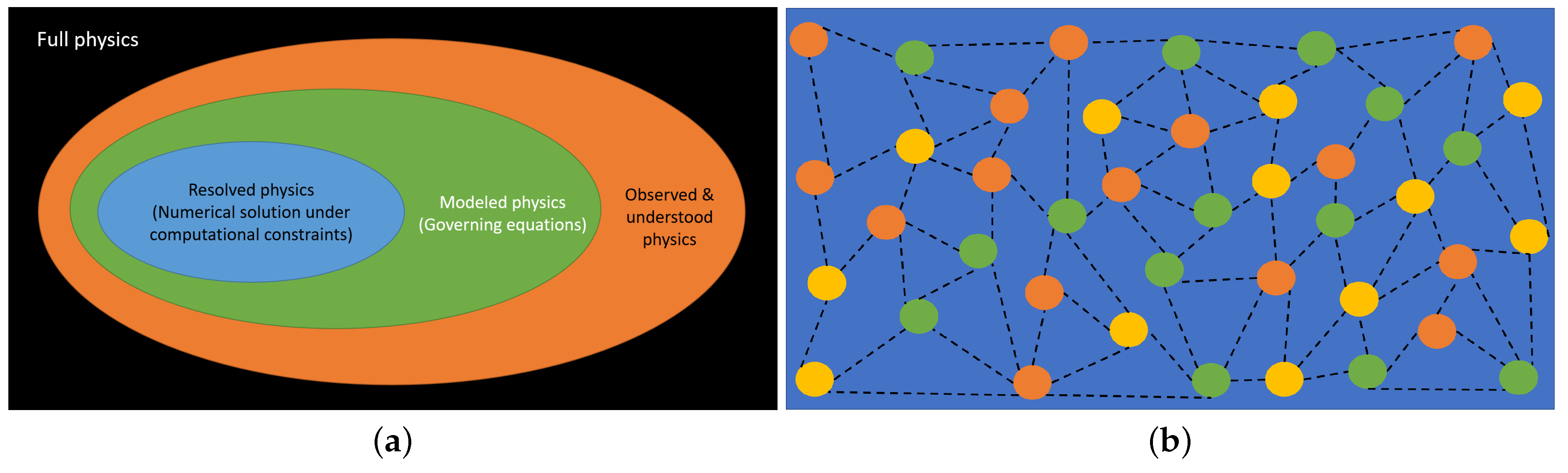
1. Introduction
2. Full Order Model (FOM)
2.1. Quasi-Geostrophic (QG) Ocean Model
2.2. Numerical Schemes
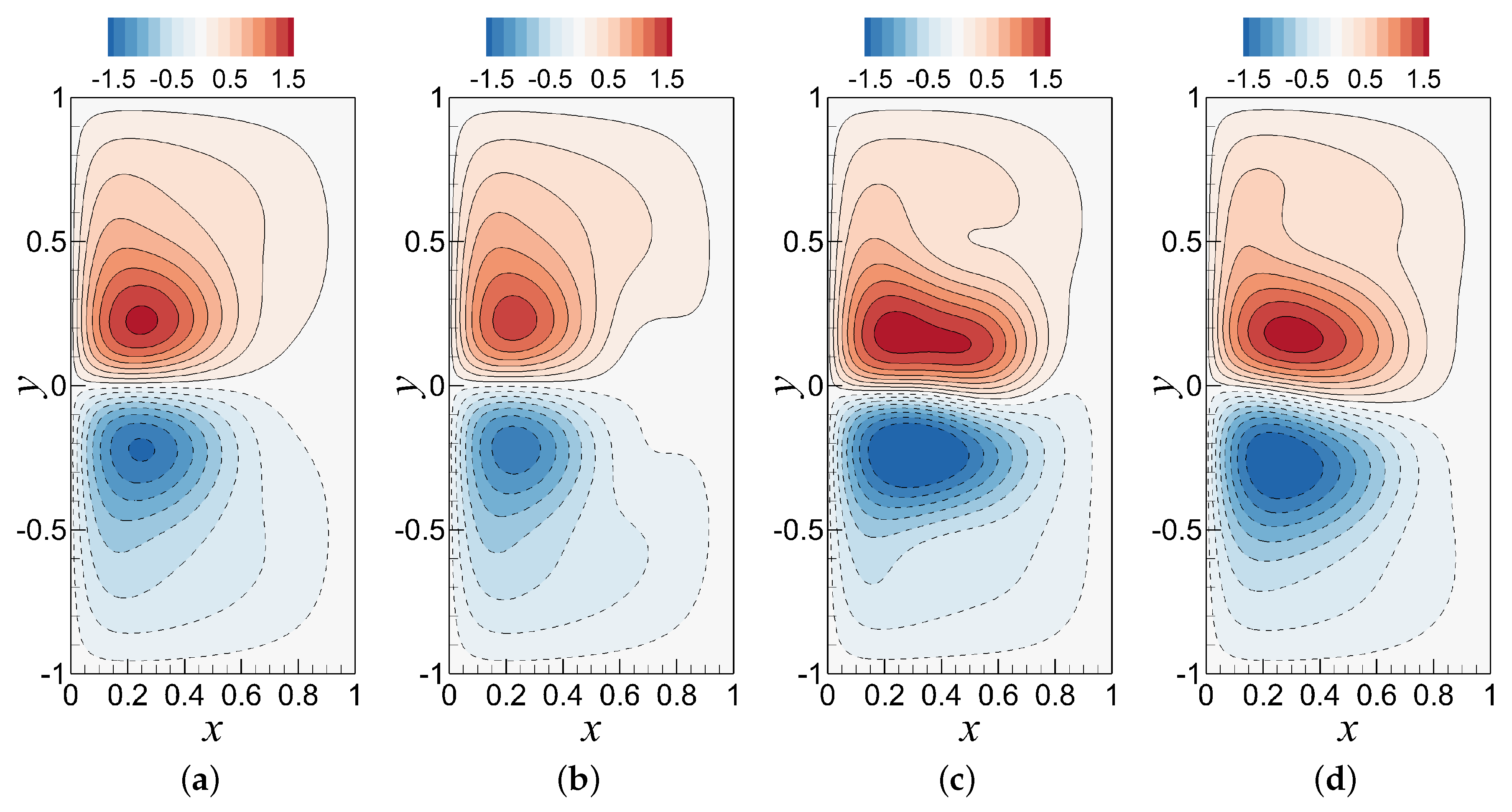
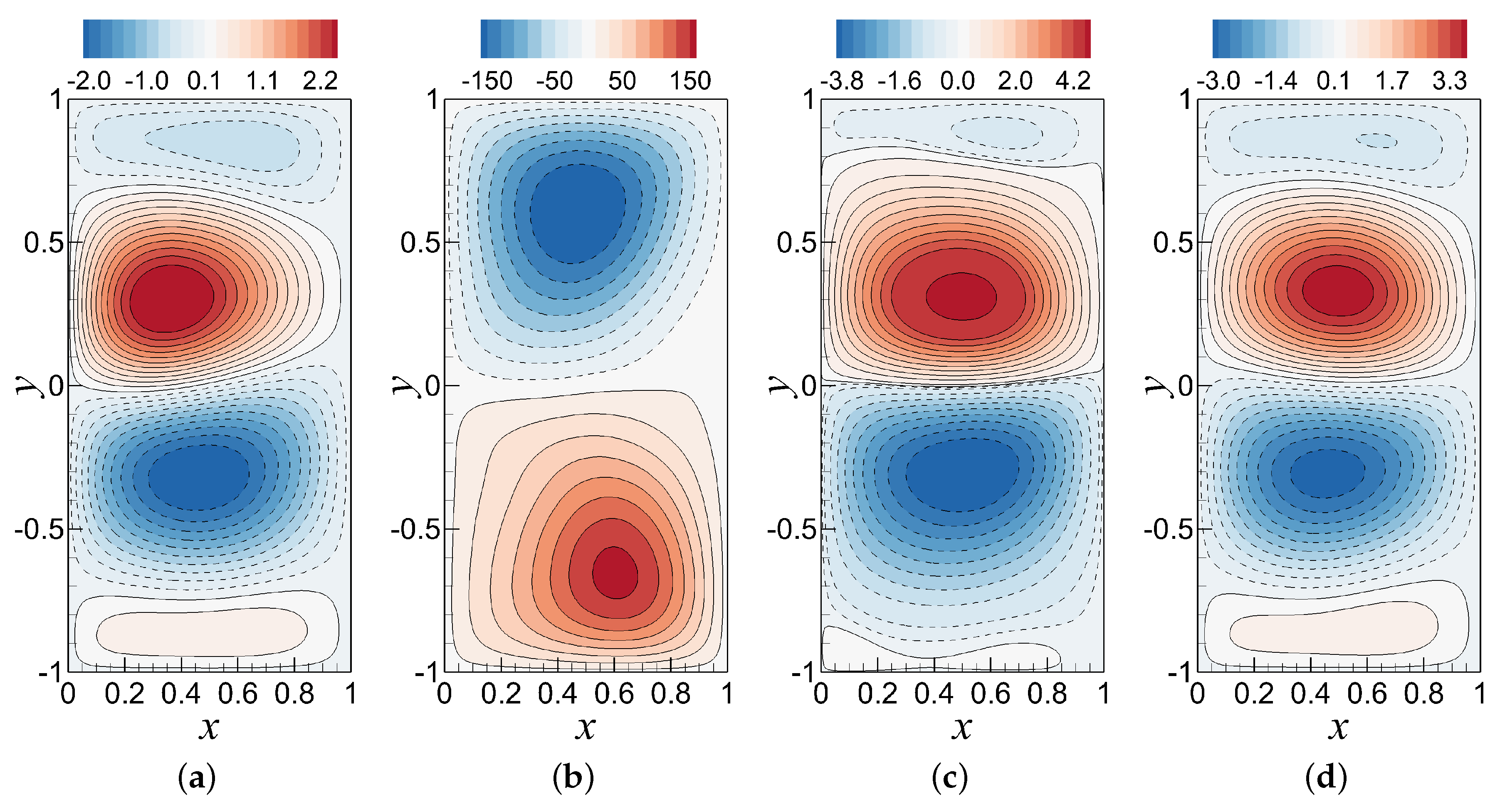
3. Galerkin Projection Based Reduced-Order Model (ROM-GP)
- POD basis construction:
- *
- Construct a data correlation matrix of the fluctuating part, from the snapshots where . Here, i and j refer to the snapshot indices.
- *
- Compute the optimal POD basis functions by solving where is the diagonal eigenvalue matrix and refers to right eigenvector matrix whose columns are eigenvectors of . In general, most of the subroutines for solving above eigenvalue equation give with all of the eigenvectors normalized to unity.
- *
- Using the eigenvalues stored in a descending order in the diagonal matrix, , define the orthogonal POD basis functions for the vorticity field aswhere is the kth eigenvalue, is the nth component of the kth eigenvector, and is the kth POD mode. We must mention that the eigenvectors must be normalized in such a way that the basis functions satisfy the orthogonality condition.
- *
- Obtain the kth mode for the stream function, , utilizing the linear dependence between stream function and vorticity given by Equation (6): .
- *
- Span the fluctuating component of the field variables into the POD modes by doing the separation of variable aswhere is the time-dependent modal coefficients and and refer to the POD modes. It should be noted that the same accounts for both stream function and vorticity based on the kinematic relation given by Equation (6).
- *
- Retain R modes where , such that these R largest energy containing modes correspond to the largest eigenvalues (). The resulting full expression for the field variables can be written as
- Galerkin projection to obtain ROM:
- *
- Perform an orthogonal Galerkin projection by multiplying the governing equation with the POD basis functions and integrating over the domain [74], which yields the following dynamical system for :where
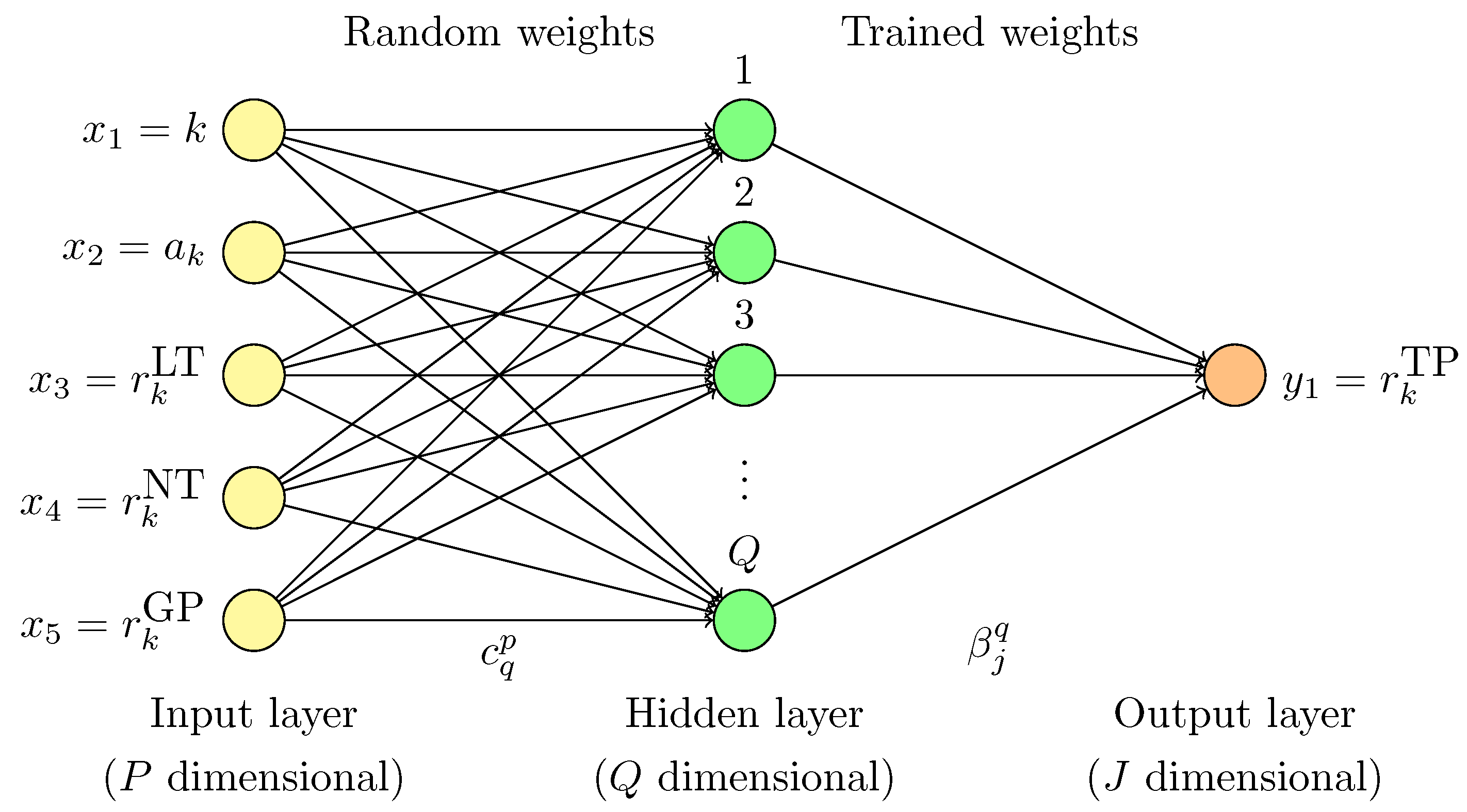
4. Artificial Neural Network Based Non-Intrusive Reduced-Order Model (ROM-ANN)
5. Hybrid Modeling (ROM-GP + ROM-ANN) Based Reduced-Order Model (ROM-H)
- Step 1 (offline):
- Generate a set of basis functions for from the snapshot data obtained from FOM.
- Step 2 (offline):
- Apply Galerkin projection to compute the coefficients required for ROM-GP.
- Step 3 (offline):
- Train the ELM network using the resolved ROM-GP coefficients and true projections datasets.
- Step 4 (online):
- Compute by solving the following ordinary differential equations in reduced-order space:where we define as a free weighting parameter in a range of to establish a relationship between the standard ROM-GP and non-intrusive ROM-ANN models. If , we recover Equation (23), whereas, for , Equation (40) can be obtained.
- Step 5 (offline):
- Obtain the full order solution by transferring data from reduced-order space by using Equation (20) as a post-processing task if needed.
6. Numerical Results
6.1. Case Setup Specifications for FOM Simulations
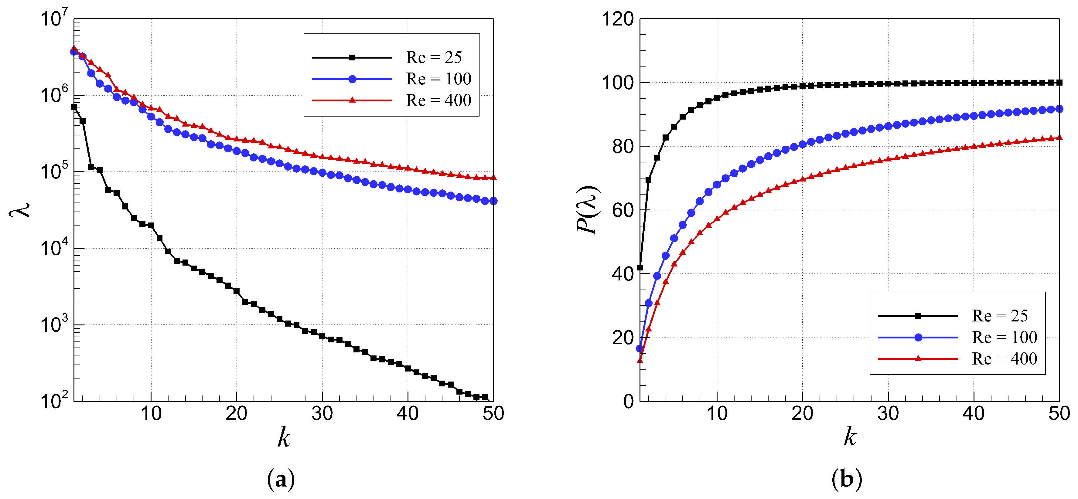
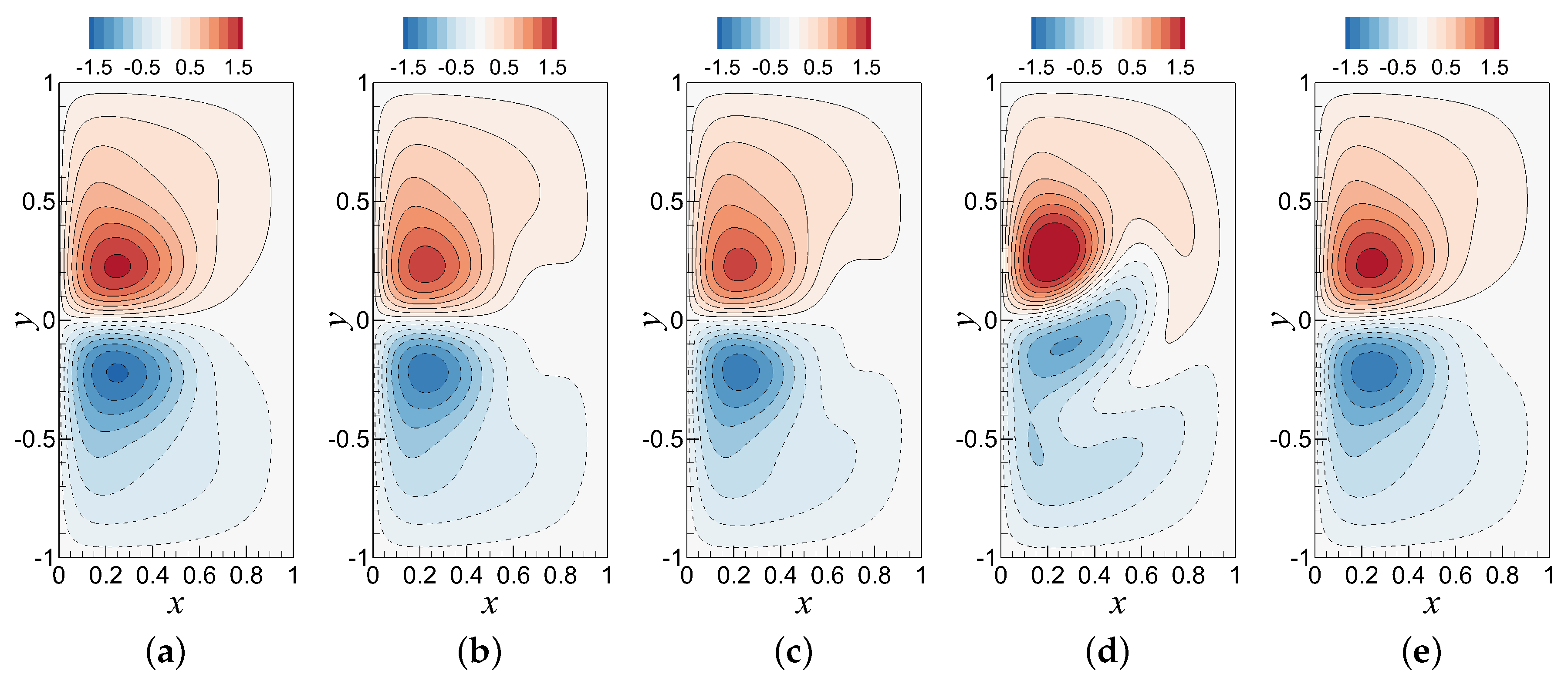
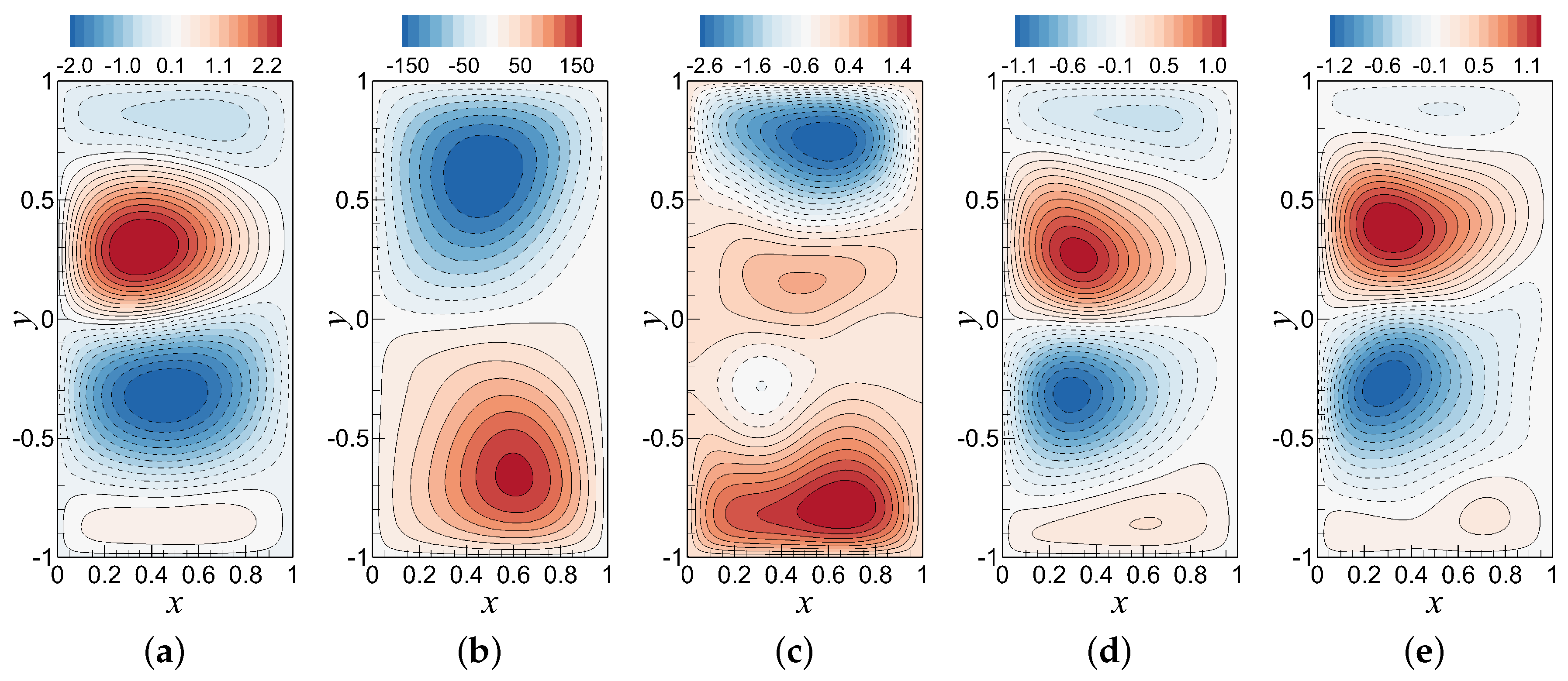
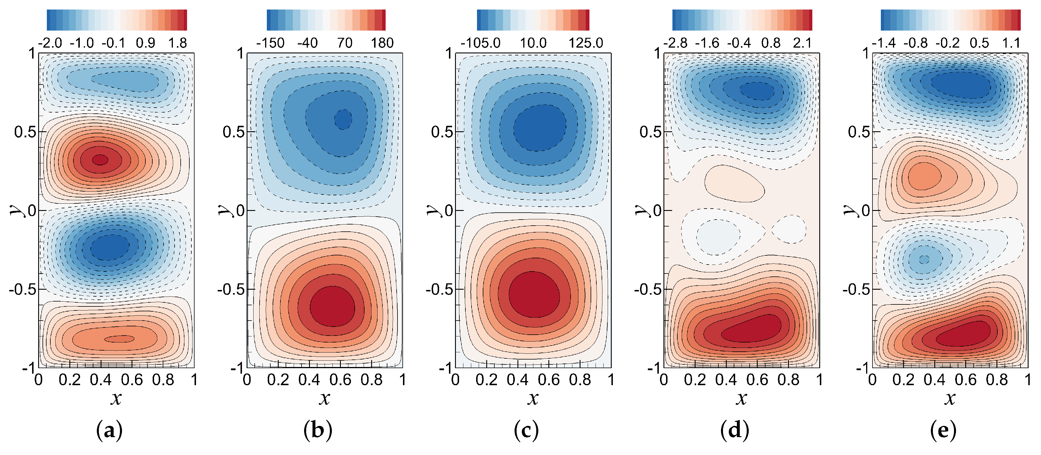
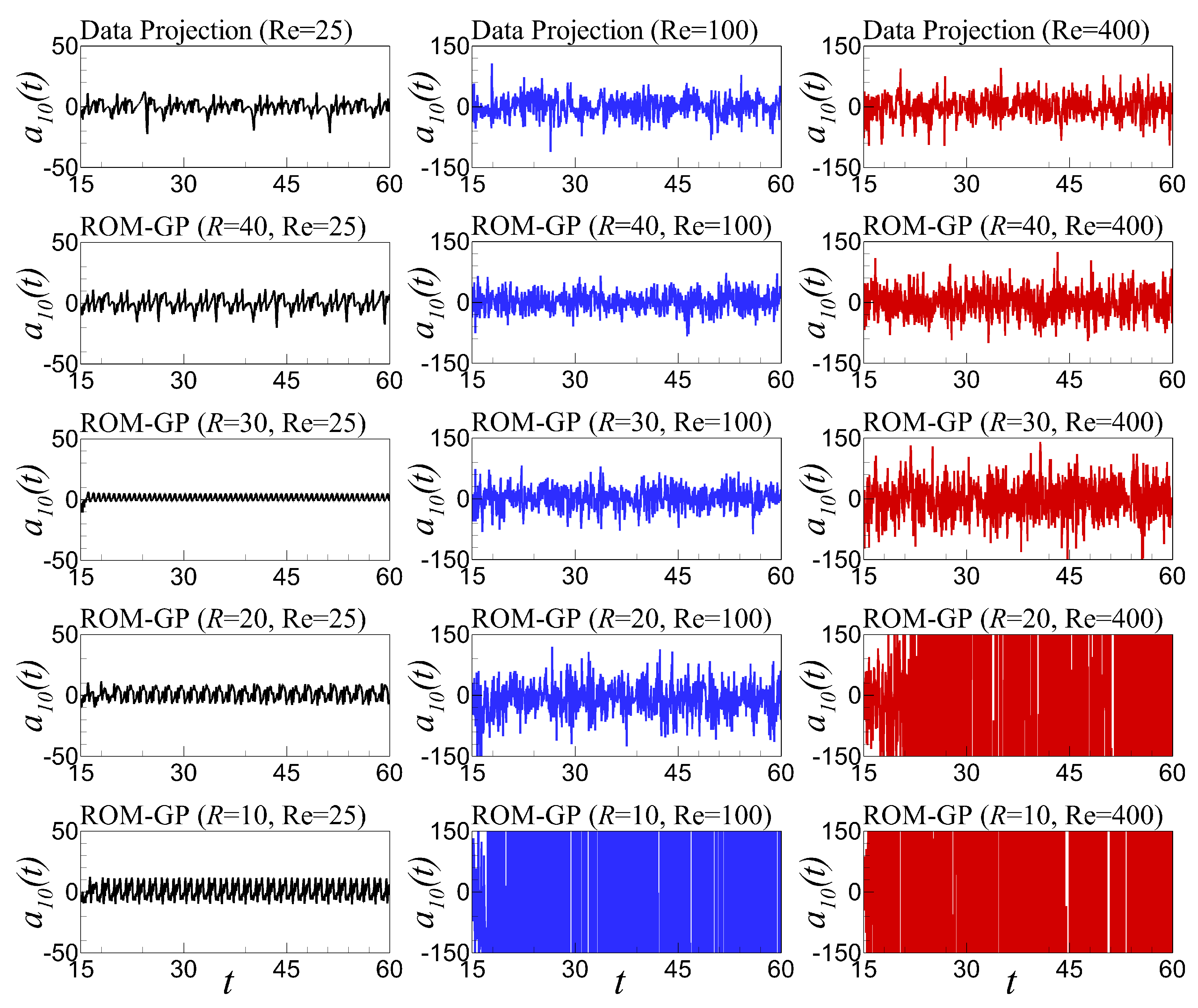
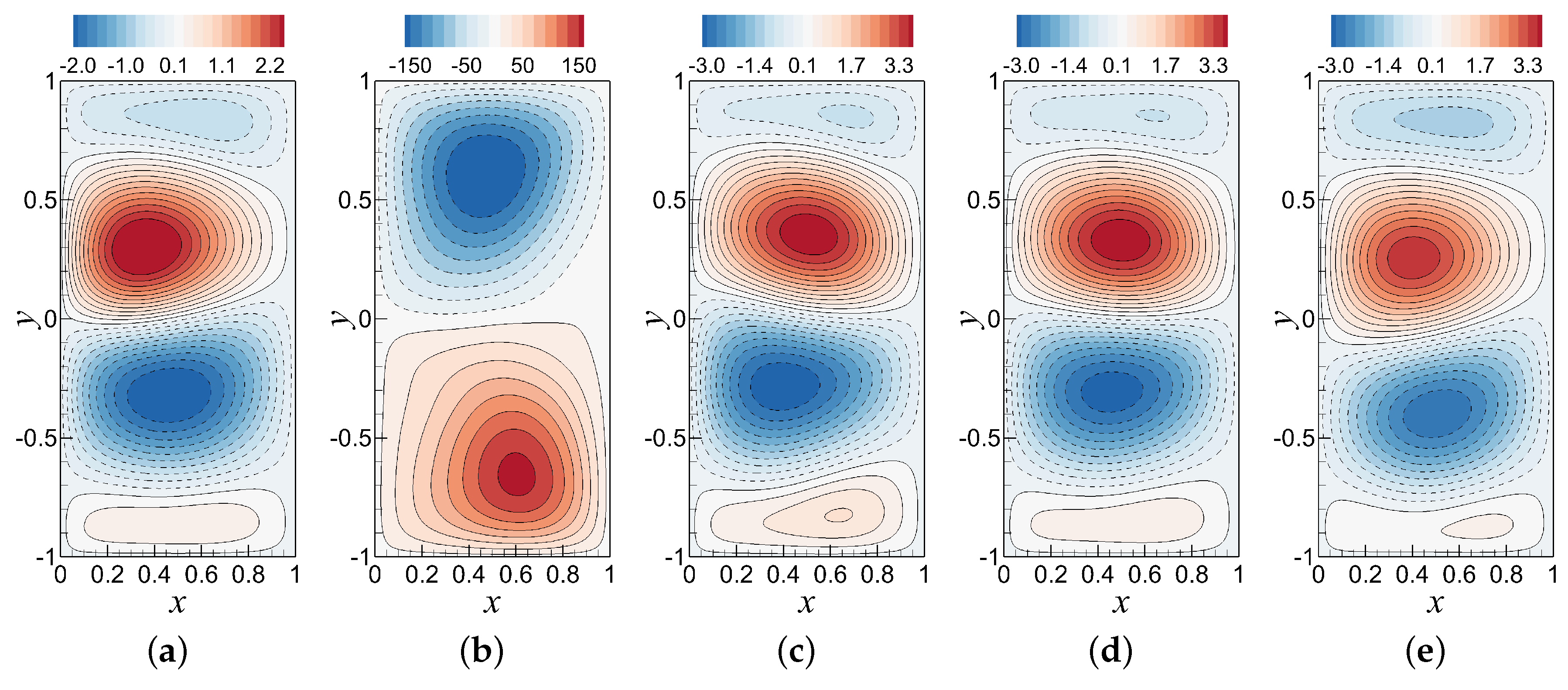
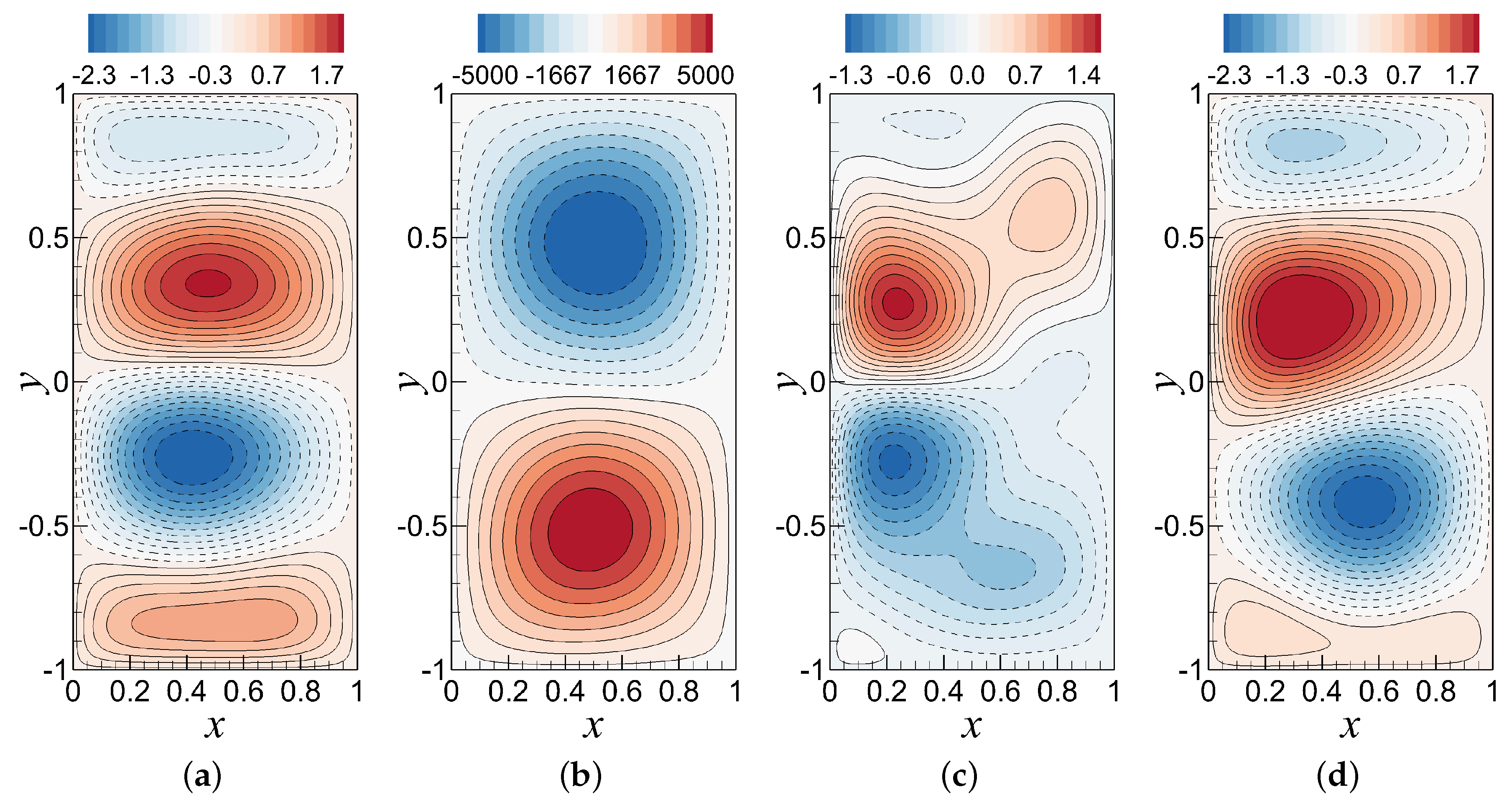
6.2. Analysis of the Standard ROM-GP Method
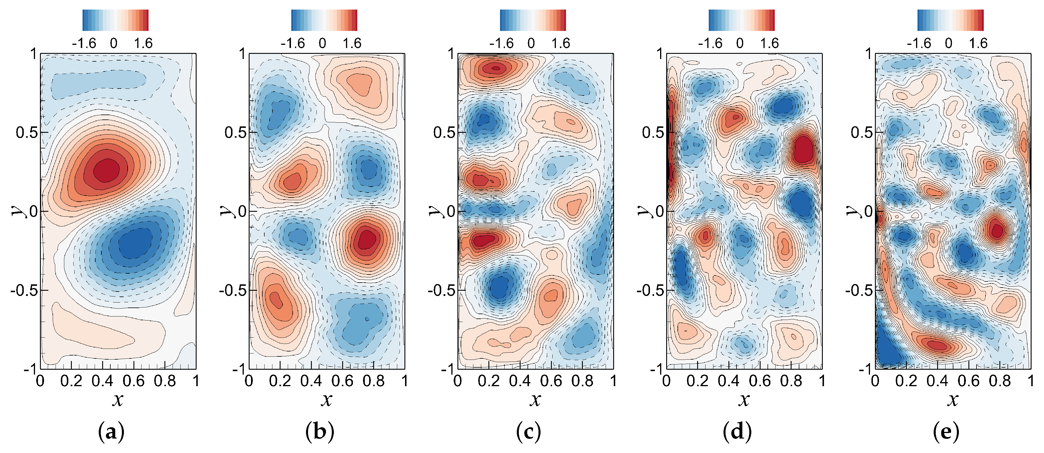
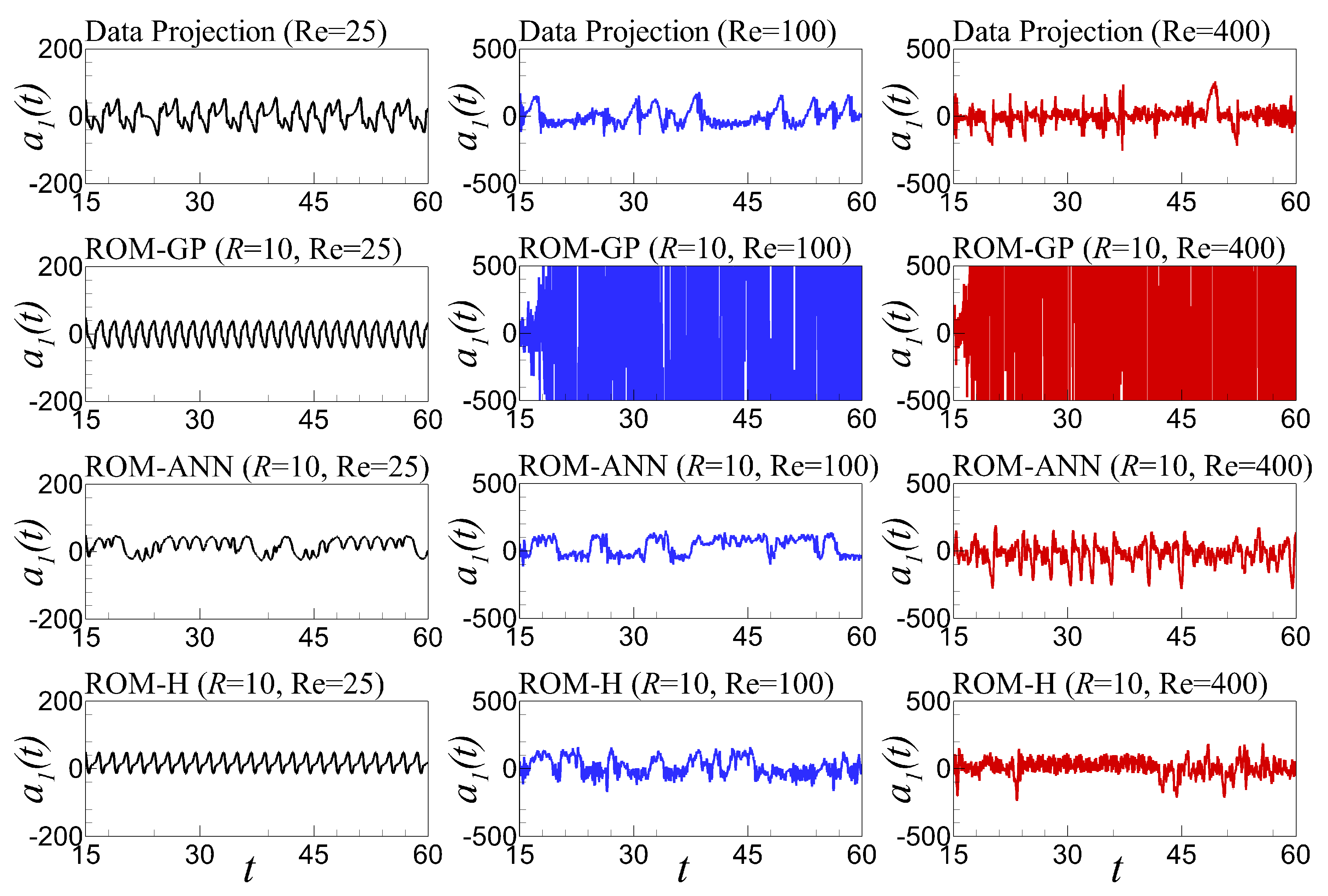
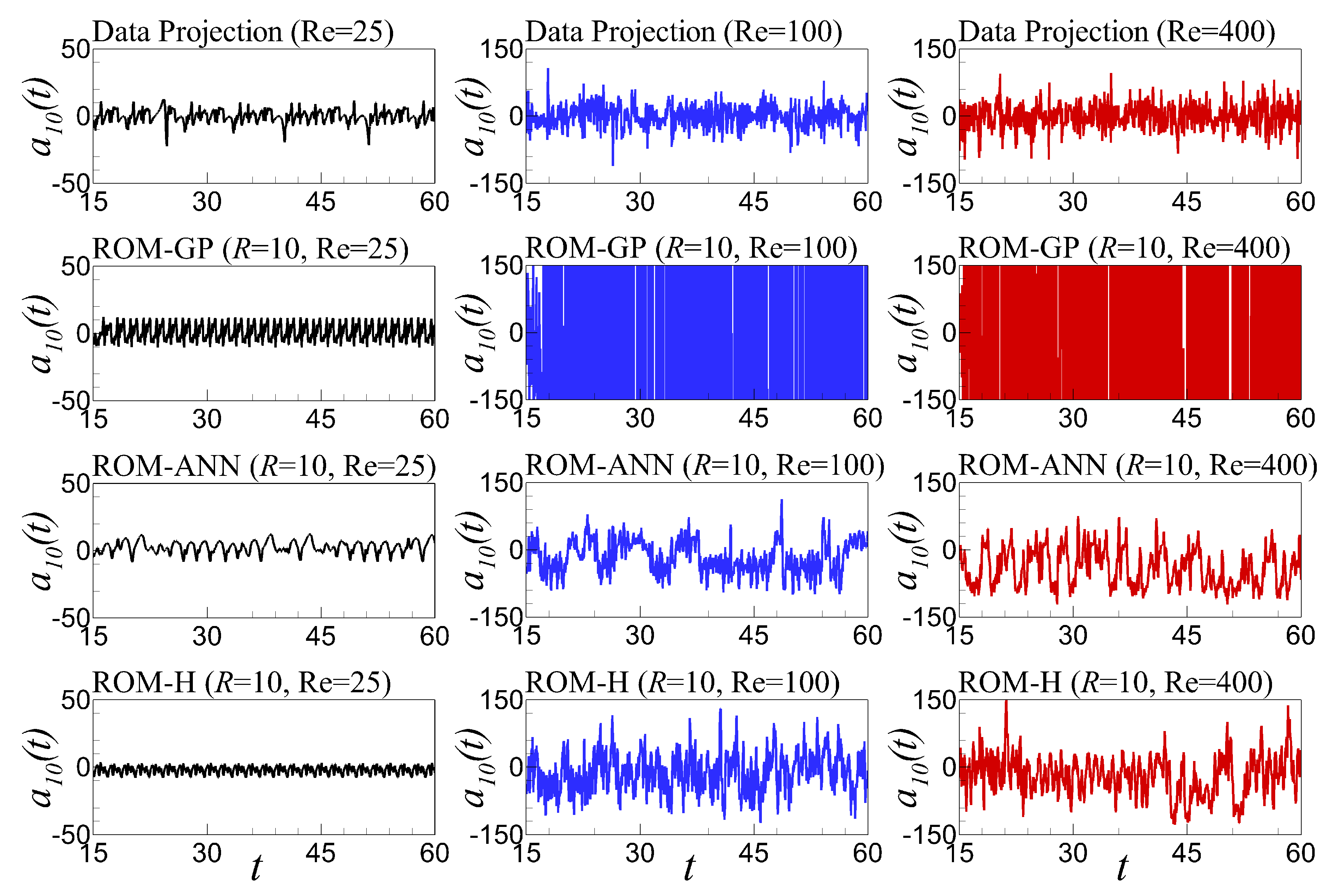
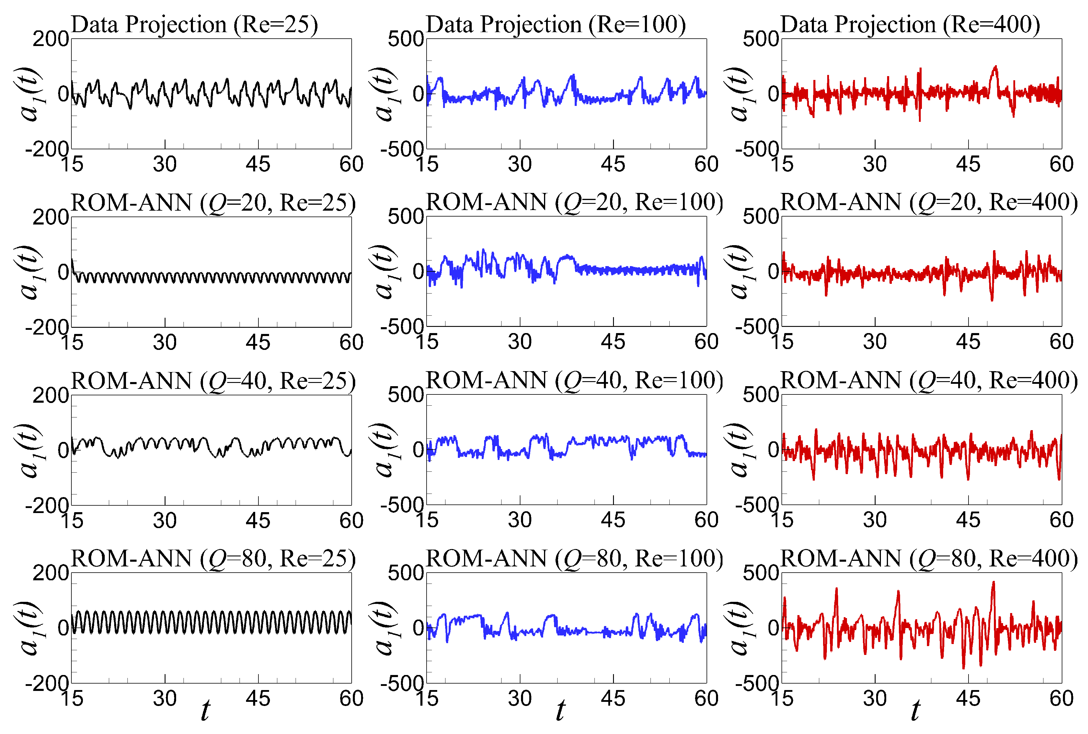
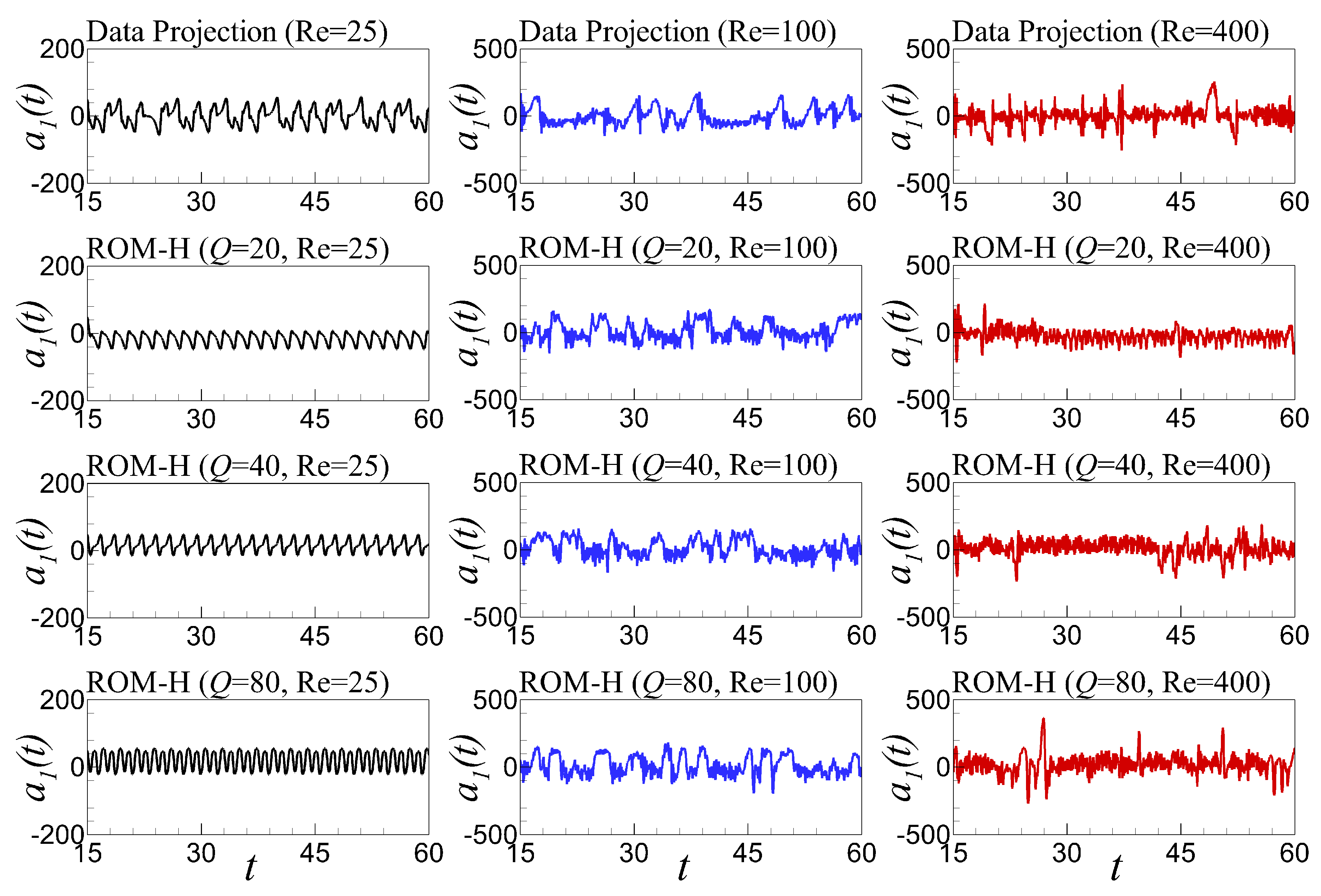
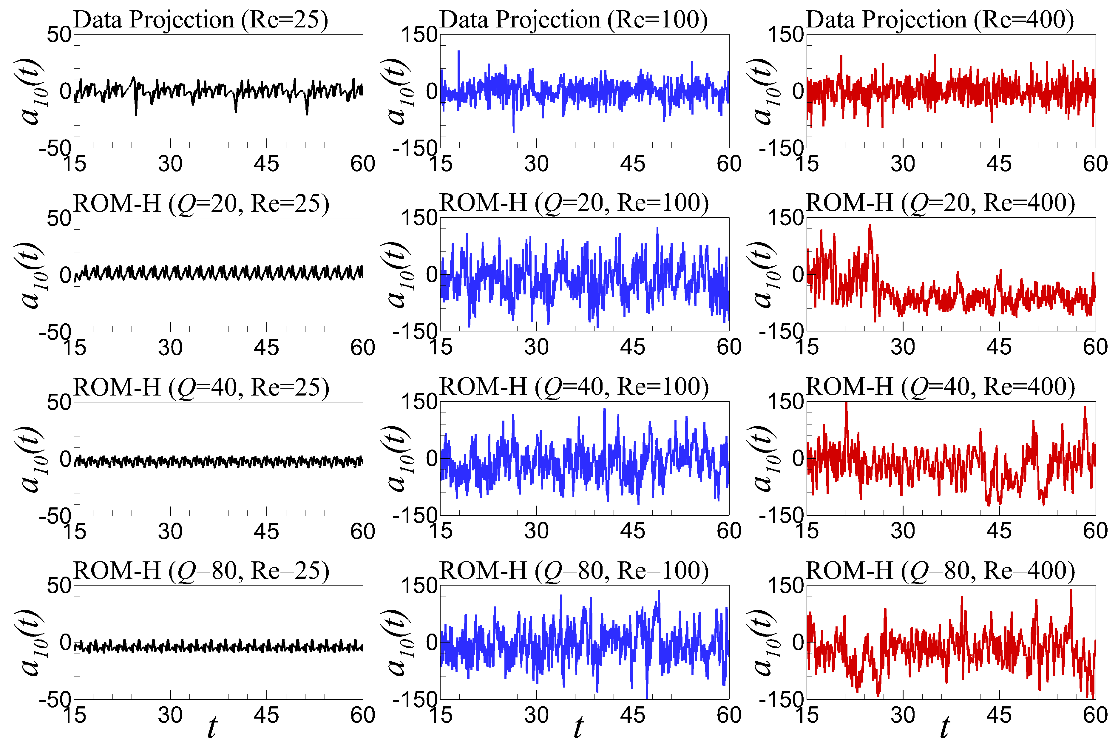
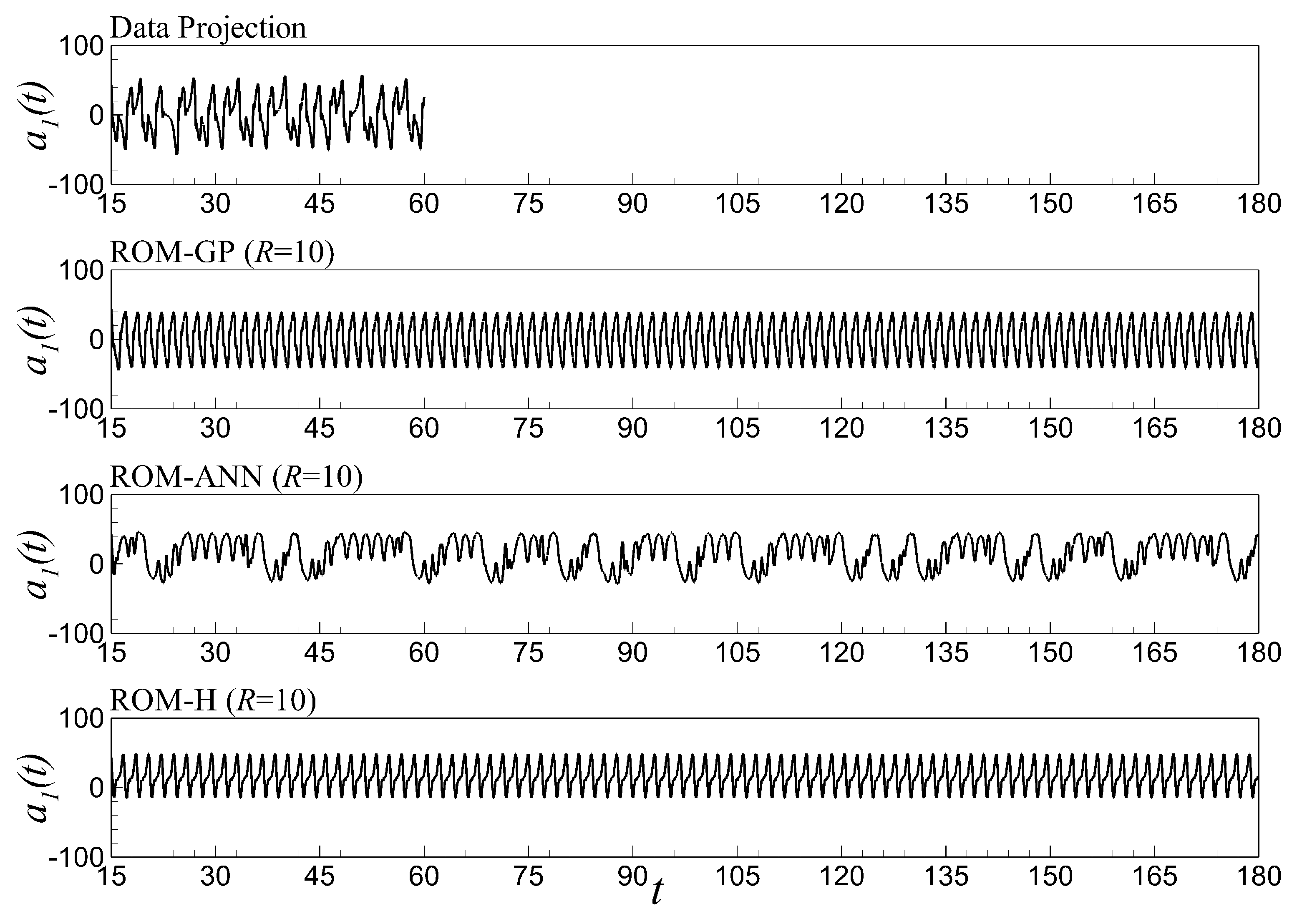
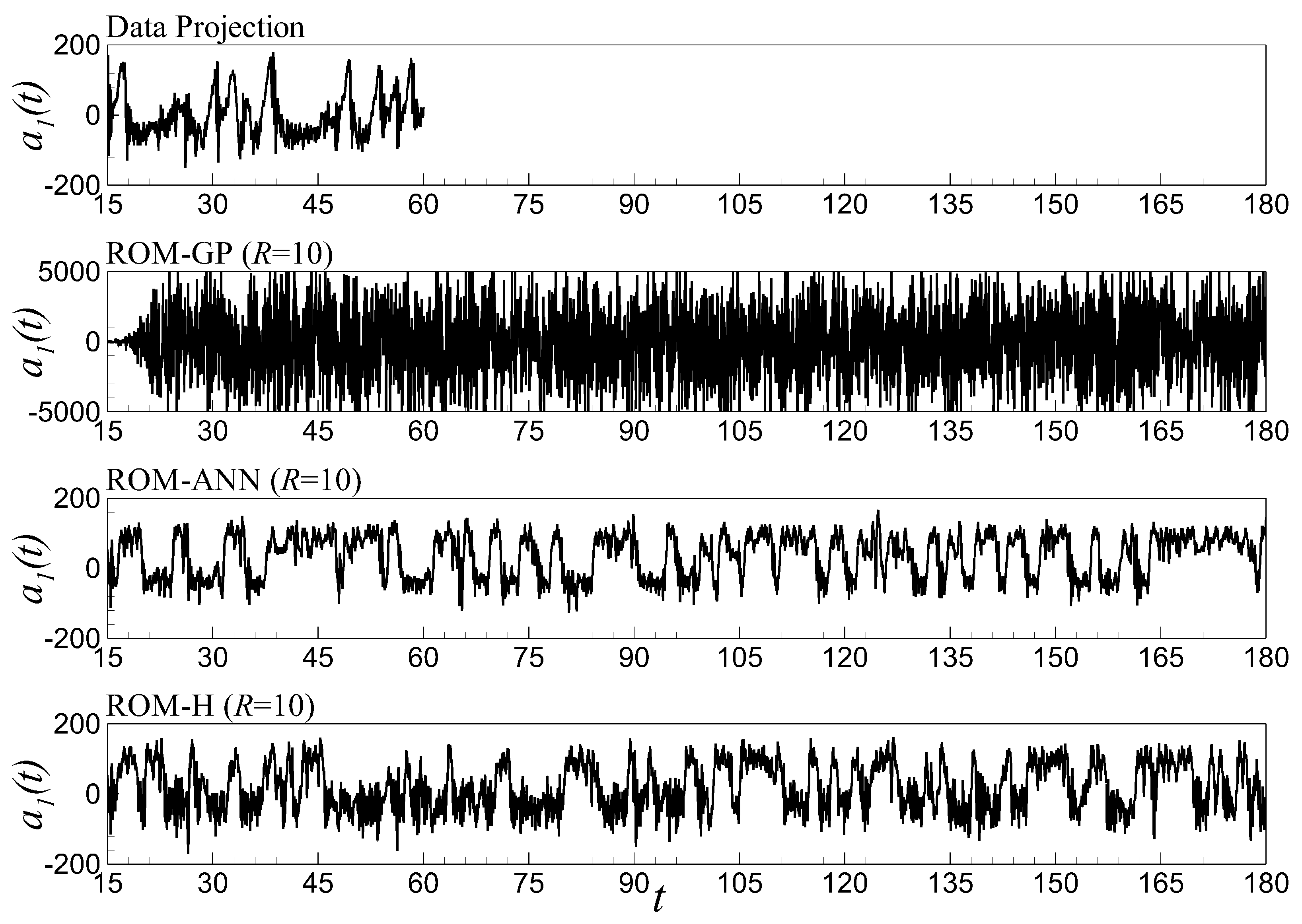
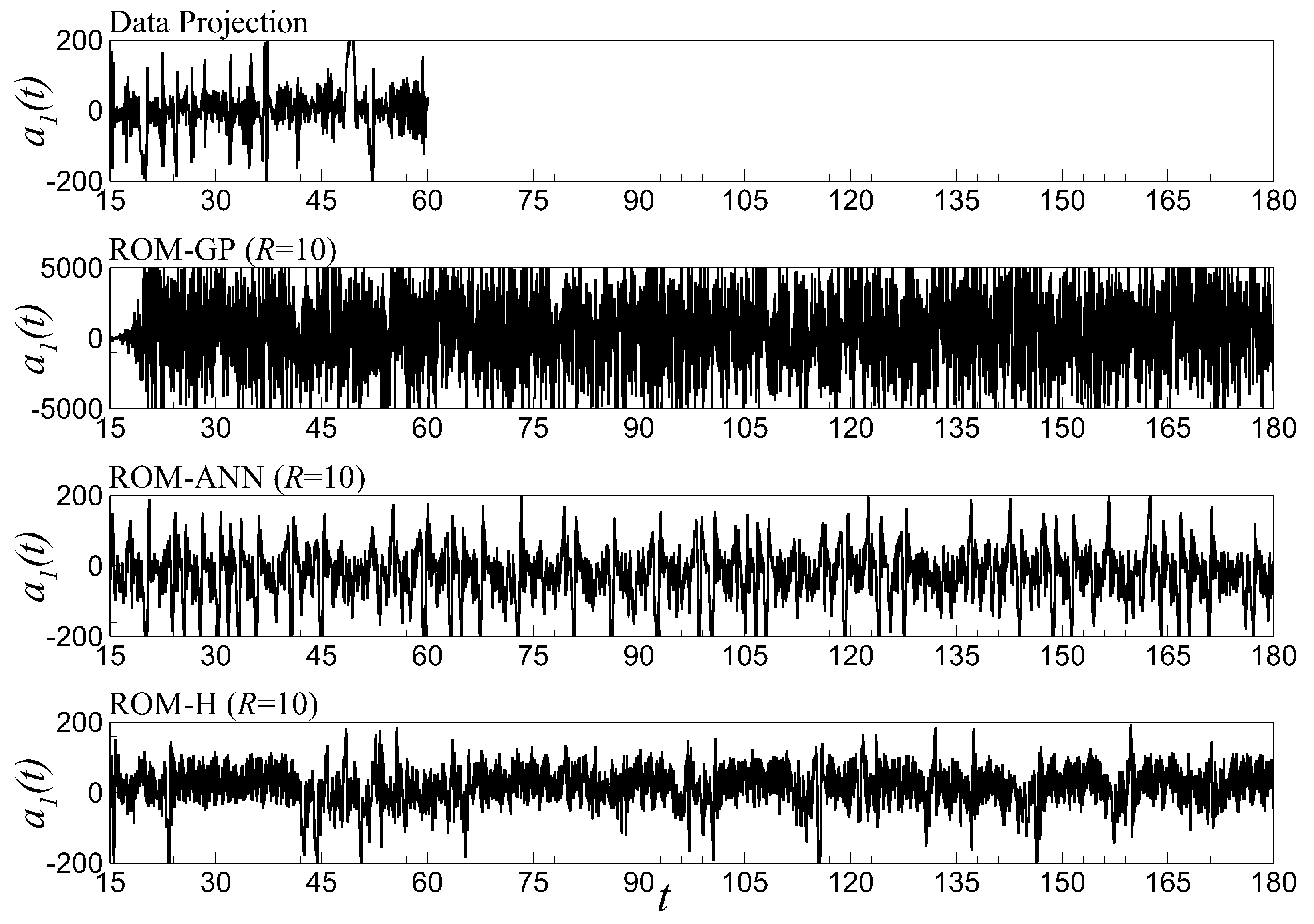
6.3. Assessments of the Prediction Performance of ROM-GP, ROM-ANN, ROM-H
6.4. Sensitivity Analysis with Respect to ELM Neurons
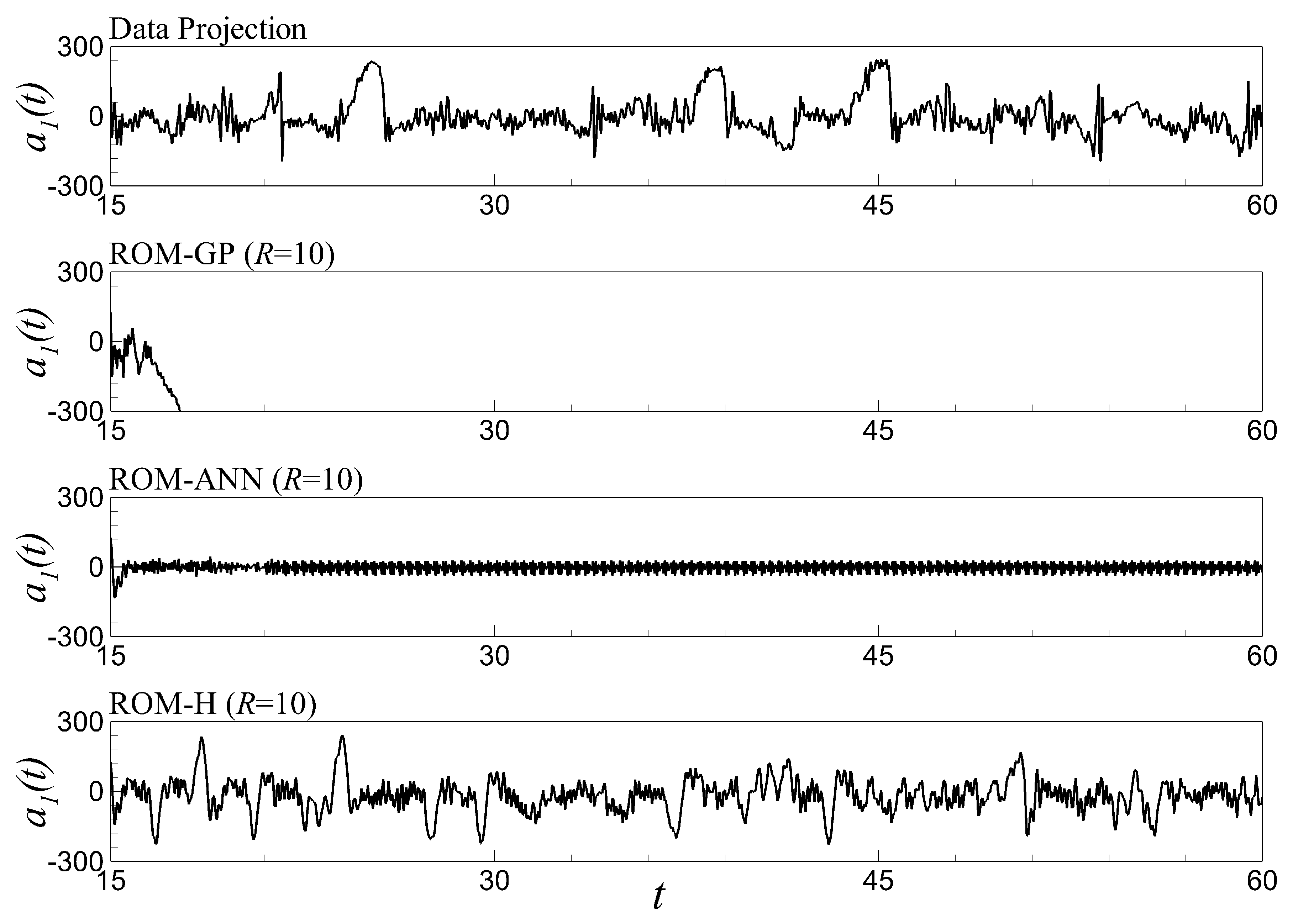
6.5. Time Series Evolution and Out-of-Sample Forecasting
7. Summary
Author Contributions
Funding
Acknowledgments
Conflicts of Interest
References
- Sagaut, P. Large Eddy Simulation for Incompressible Flows: An Introduction; Springer Science & Business Media: Berlin, Germany, 2006. [Google Scholar]
- Wilcox, D.C. Turbulence Modeling for CFD; DCW Industries: La Canada Flintridge, CA, USA, 1998. [Google Scholar]
- Durbin, P.A. Some recent developments in turbulence closure modeling. Ann. Rev. Fluid Mech. 2018, 50, 77–103. [Google Scholar] [CrossRef]
- Duraisamy, K.; Iaccarino, G.; Xiao, H. Turbulence modeling in the age of data. arXiv, 2018; arXiv:1804.00183. [Google Scholar]
- Munk, W.H. On the wind-driven ocean circulation. J. Meteorol. 1950, 7, 80–93. [Google Scholar] [CrossRef]
- Pelc, R.; Fujita, R.M. Renewable energy from the ocean. Mar. Policy 2002, 26, 471–479. [Google Scholar] [CrossRef]
- Esteban, M.; Leary, D. Current developments and future prospects of offshore wind and ocean energy. Appl. Energy 2012, 90, 128–136. [Google Scholar] [CrossRef]
- McWilliams, J.C. Fundamentals of Geophysical Fluid Dynamics; Cambridge University Press: New York, NY, USA, 2006. [Google Scholar]
- Berloff, P. Dynamically consistent parameterization of mesoscale eddies. Part I: Simple model. Ocean Model. 2015, 87, 1–19. [Google Scholar] [CrossRef]
- San, O.; Staples, A.E.; Wang, Z.; Iliescu, T. Approximate deconvolution large eddy simulation of a barotropic ocean circulation model. Ocean Model. 2011, 40, 120–132. [Google Scholar] [CrossRef]
- Berloff, P. Dynamically consistent parameterization of mesoscale eddies—Part II: Eddy fluxes and diffusivity from transient impulses. Fluids 2016, 1, 22. [Google Scholar] [CrossRef]
- Miller, R.N. Numerical Modeling of Ocean Circulation; Cambridge University Press: New York, NY, USA, 2007. [Google Scholar]
- Kondrashov, D.; Chekroun, M.D.; Berloff, P. Multiscale Stuart–Landau emulators: Application to wind-driven ocean gyres. Fluids 2018, 3, 21. [Google Scholar] [CrossRef]
- Lynch, P. The origins of computer weather prediction and climate modeling. J. Comput. Phys. 2008, 227, 3431–3444. [Google Scholar] [CrossRef]
- Laurie, J.; Bouchet, F. Computation of rare transitions in the barotropic quasi-geostrophic equations. New J. Phys. 2015, 17, 015009. [Google Scholar] [CrossRef]
- Rowley, C.W.; Dawson, S.T. Model reduction for flow analysis and control. Ann. Rev. Fluid Mech. 2017, 49, 387–417. [Google Scholar] [CrossRef]
- Taira, K.; Brunton, S.L.; Dawson, S.T.; Rowley, C.W.; Colonius, T.; McKeon, B.J.; Schmidt, O.T.; Gordeyev, S.; Theofilis, V.; Ukeiley, L.S. Modal analysis of fluid flows: An overview. AIAA J. 2017, 55, 4013–4041. [Google Scholar] [CrossRef]
- Ito, K.; Ravindran, S. A reduced-order method for simulation and control of fluid flows. J. Comput. Phys. 1998, 143, 403–425. [Google Scholar] [CrossRef]
- Lucia, D.J.; Beran, P.S.; Silva, W.A. Reduced-order modeling: New approaches for computational physics. Prog. Aerosp. Sci. 2004, 40, 51–117. [Google Scholar] [CrossRef]
- Brenner, T.A.; Fontenot, R.L.; Cizmas, P.G.; O’Brien, T.J.; Breault, R.W. A reduced-order model for heat transfer in multiphase flow and practical aspects of the proper orthogonal decomposition. Comput. Chem. Eng. 2012, 43, 68–80. [Google Scholar] [CrossRef]
- Iollo, A.; Lanteri, S.; Désidéri, J.A. Stability properties of POD–Galerkin approximations for the compressible Navier–Stokes equations. Theor. Comput. Fluid Dyn. 2000, 13, 377–396. [Google Scholar] [CrossRef]
- Freno, B.A.; Cizmas, P.G. A proper orthogonal decomposition method for nonlinear flows with deforming meshes. Int. J. Heat Fluid Flow 2014, 50, 145–159. [Google Scholar] [CrossRef]
- San, O.; Iliescu, T. A stabilized proper orthogonal decomposition reduced-order model for large scale quasigeostrophic ocean circulation. Adv. Comput. Math. 2015, 41, 1289–1319. [Google Scholar] [CrossRef]
- Behzad, F.; Helenbrook, B.T.; Ahmadi, G. On the sensitivity and accuracy of proper-orthogonal-decomposition-based reduced order models for Burgers equation. Comput. Fluids 2015, 106, 19–32. [Google Scholar] [CrossRef]
- Cizmas, P.G.; Richardson, B.R.; Brenner, T.A.; O’Brien, T.J.; Breault, R.W. Acceleration techniques for reduced-order models based on proper orthogonal decomposition. J. Comput. Phys. 2008, 227, 7791–7812. [Google Scholar] [CrossRef]
- Bistrian, D.; Navon, I. An improved algorithm for the shallow water equations model reduction: Dynamic Mode Decomposition vs. POD. Int. J. Numer. Methods Fluids 2015, 78, 552–580. [Google Scholar] [CrossRef]
- Behzad, F.; Helenbrook, B.T.; Ahmadi, G. Multilevel Algorithm for Obtaining the Proper Orthogonal Decomposition. AIAA J. 2018. [Google Scholar] [CrossRef]
- Bistrian, D.A.; Navon, I.M. Randomized dynamic mode decomposition for nonintrusive reduced order modelling. Int. J. Numer. Methods Eng. 2017, 112, 3–25. [Google Scholar] [CrossRef]
- Gautier, N.; Aider, J.L.; Duriez, T.; Noack, B.; Segond, M.; Abel, M. Closed-loop separation control using machine learning. J. Fluid Mech. 2015, 770, 442–457. [Google Scholar] [CrossRef]
- Lee, C.; Kim, J.; Babcock, D.; Goodman, R. Application of neural networks to turbulence control for drag reduction. Phys. Fluids 1997, 9, 1740–1747. [Google Scholar] [CrossRef]
- Gamahara, M.; Hattori, Y. Searching for turbulence models by artificial neural network. Phys. Rev. Fluids 2017, 2, 054604. [Google Scholar] [CrossRef]
- Duraisamy, K.; Zhang, Z.J.; Singh, A.P. New approaches in turbulence and transition modeling using data-driven techniques. In Proceedings of the 53rd AIAA Aerospace Sciences Meeting, Kissimmee, FL, USA, 5–9 January 2015; p. 1284. [Google Scholar]
- Maulik, R.; San, O. A neural network approach for the blind deconvolution of turbulent flows. J. Fluid Mech. 2017, 831, 151–181. [Google Scholar] [CrossRef]
- San, O.; Maulik, R. Extreme learning machine for reduced order modeling of turbulent geophysical flows. Phys. Rev. E 2018, 97, 042322. [Google Scholar] [CrossRef] [PubMed]
- Wu, J.L.; Xiao, H.; Paterson, E. Physics-informed machine learning approach for augmenting turbulence models: A comprehensive framework. Phys. Rev. Fluids 2018, 3, 074602. [Google Scholar] [CrossRef]
- Moosavi, A.; Stefanescu, R.; Sandu, A. Efficient construction of local parametric reduced order models using machine learning techniques. arXiv, 2015; arXiv:1511.02909. [Google Scholar]
- Huang, G.B.; Zhu, Q.Y.; Siew, C.K. Extreme learning machine: Theory and applications. Neurocomputing 2006, 70, 489–501. [Google Scholar] [CrossRef]
- Huang, G.B.; Chen, L. Convex incremental extreme learning machine. Neurocomputing 2007, 70, 3056–3062. [Google Scholar] [CrossRef]
- Xiang, J.; Westerlund, M.; Sovilj, D.; Pulkkis, G. Using extreme learning machine for intrusion detection in a big data environment. In Proceedings of the 2014 Workshop on Artificial Intelligent and Security Workshop, Scottsdale, AZ, USA, 3–7 November 2014; pp. 73–82. [Google Scholar]
- Williams, M.O.; Schmid, P.J.; Kutz, J.N. Hybrid reduced-order integration with proper orthogonal decomposition and dynamic mode decomposition. Multiscale Model. Simul. 2013, 11, 522–544. [Google Scholar] [CrossRef]
- Xie, X.; Mohebujjaman, M.; Rebholz, L.; Iliescu, T. Data-driven filtered reduced order modeling of fluid flows. SIAM J. Sci. Comput. 2018, 40, B834–B857. [Google Scholar] [CrossRef]
- Mohebujjaman, M.; Rebholz, L.; Iliescu, T. Physically-constrained data-driven, filtered reduced order modeling of fluid flows. arXiv, 2018; arXiv:1806.0035. [Google Scholar]
- Wan, Z.Y.; Vlachas, P.; Koumoutsakos, P.; Sapsis, T. Data-assisted reduced-order modeling of extreme events in complex dynamical systems. PLoS ONE 2018, 13, e0197704. [Google Scholar] [CrossRef] [PubMed]
- Pathak, J.; Wikner, A.; Fussell, R.; Chandra, S.; Hunt, B.R.; Girvan, M.; Ott, E. Hybrid forecasting of chaotic processes: Using machine learning in conjunction with a knowledge-based model. Chao Interdiscip. J. Nonlinear Sci. 2018, 28, 041101. [Google Scholar] [CrossRef]
- Siedler, G.; Griffies, S.M.; Gould, J.; Church, J.A. Ocean Circulation and Climate: A 21st Century Perspective; Academic Press: Cambridge, MA, USA, 2013; Volume 103. [Google Scholar]
- Byrne, D.; Münnich, M.; Frenger, I.; Gruber, N. Mesoscale atmosphere ocean coupling enhances the transfer of wind energy into the ocean. Nat. Commun. 2016, 7, ncomms11867. [Google Scholar] [CrossRef] [PubMed]
- Holland, W.R. The role of mesoscale eddies in the general circulation of the ocean—Numerical experiments using a wind-driven quasi-geostrophic model. J. Phys. Oceanogr. 1978, 8, 363–392. [Google Scholar] [CrossRef]
- Hogg, A.M.C.; Dewar, W.K.; Berloff, P.; Kravtsov, S.; Hutchinson, D.K. The effects of mesoscale ocean–atmosphere coupling on the large-scale ocean circulation. J. Clim. 2009, 22, 4066–4082. [Google Scholar] [CrossRef]
- Hua, B.; Haidvogel, D. Numerical simulations of the vertical structure of quasi-geostrophic turbulence. J. Atmos. Sci. 1986, 43, 2923–2936. [Google Scholar] [CrossRef]
- Ghil, M.; Chekroun, M.D.; Simonnet, E. Climate dynamics and fluid mechanics: Natural variability and related uncertainties. Phys. D Nonlinear Phenom. 2008, 237, 2111–2126. [Google Scholar] [CrossRef]
- Charney, J.G.; Fjörtoft, R.; Neumann, J.V. Numerical integration of the barotropic vorticity equation. Tellus 1950, 2, 237–254. [Google Scholar] [CrossRef]
- Bouchet, F.; Simonnet, E. Random changes of flow topology in two-dimensional and geophysical turbulence. Phys. Rev. Lett. 2009, 102, 094504. [Google Scholar] [CrossRef] [PubMed]
- Cushman-Roisin, B.; Beckers, J.M. Introduction to Geophysical Fluid Dynamics: Physical and Numerical Aspects; Academic Press: Waltham, MA, USA, 2011. [Google Scholar]
- Majda, A.; Wang, X. Nonlinear Dynamics and Statistical Theories for Basic Geophysical Flows; Cambridge University Press: New York, NY, USA, 2006. [Google Scholar]
- Vallis, G.K. Atmospheric and Oceanic Fluid Dynamics; Cambridge University Press: New York, NY, USA, 2017. [Google Scholar]
- Greatbatch, R.J.; Nadiga, B.T. Four-gyre circulation in a barotropic model with double-gyre wind forcing. J. Phys. Oceanogr. 2000, 30, 1461–1471. [Google Scholar] [CrossRef]
- Nadiga, B.T.; Margolin, L.G. Dispersive–dissipative eddy parameterization in a barotropic model. J. Phys. Oceanogr. 2001, 31, 2525–2531. [Google Scholar] [CrossRef]
- San, O. Numerical assessments of ocean energy extraction from western boundary currents using a quasi-geostrophic ocean circulation model. Int. J. Mar. Energy 2016, 16, 12–29. [Google Scholar] [CrossRef]
- San, O.; Staples, A.E. An efficient coarse grid projection method for quasigeostrophic models of large-scale ocean circulation. Int. J. Multiscale Comput. Eng. 2013, 11, 463–495. [Google Scholar] [CrossRef]
- Özgökmen, T.M.; Chassignet, E.P. Emergence of inertial gyres in a two-layer quasigeostrophic ocean model. J. Phys. Oceanogr. 1998, 28, 461–484. [Google Scholar] [CrossRef]
- Holm, D.D.; Nadiga, B.T. Modeling mesoscale turbulence in the barotropic double-gyre circulation. J. Phys. Oceanogr. 2003, 33, 2355–2365. [Google Scholar] [CrossRef]
- Medjo, T.T. Numerical simulations of a two-layer quasi-geostrophic equation of the ocean. SIAM J. Numer. Anal. 2000, 37, 2005–2022. [Google Scholar] [CrossRef]
- Arakawa, A. Computational design for long-term numerical integration of the equations of fluid motion: Two-dimensional incompressible flow. Part I. J. Comput. Phys. 1966, 1, 119–143. [Google Scholar] [CrossRef]
- Gottlieb, S.; Shu, C.W. Total variation diminishing Runge–Kutta schemes. Math. Comput. Am. Math. Soc. 1998, 67, 73–85. [Google Scholar] [CrossRef]
- Wedi, N.P. Increasing horizontal resolution in numerical weather prediction and climate simulations: Illusion or panacea? Philos. Trans. R. Soc. A 2014, 372, 20130289. [Google Scholar] [CrossRef] [PubMed]
- Brunton, S.L.; Noack, B.R. Closed-loop turbulence control: Progress and challenges. Appl. Mech. Rev. 2015, 67, 050801. [Google Scholar] [CrossRef]
- Navon, I.M.; Zou, X.; Derber, J.; Sela, J. Variational data assimilation with an adiabatic version of the NMC spectral model. Mon. Weather Rev. 1992, 120, 1433–1446. [Google Scholar] [CrossRef]
- Kalnay, E. Atmospheric Modeling, Data Assimilation and Predictability; Cambridge University Press: Cambridge, UK, 2003. [Google Scholar]
- Holmes, P.; Lumley, J.L.; Berkooz, G.; Rowley, C.W. Turbulence, Coherent Structures, Dynamical Systems and Symmetry; Cambridge University Press: New York, NY, USA, 2012. [Google Scholar]
- Lumley, J.L. Stochastic Tools in Turbulence; Academic Press: New York, NY, USA, 1970. [Google Scholar]
- Kosambi, D.D. Statistics in function space. In D D Kosambi; Ramaswamy, R., Ed.; Springer: New Delhi, India, 2016; pp. 115–123. [Google Scholar]
- Sirovich, L. Turbulence and the dynamics of coherent structures. I. Coherent structures. Q. Appl. Math. 1987, 45, 561–571. [Google Scholar] [CrossRef]
- Noack, B.R.; Afanasiev, K.; Morzński, M.; Tadmor, G.; Thiele, F. A hierarchy of low-dimensional models for the transient and post-transient cylinder wake. J. Fluid Mech. 2003, 497, 335–363. [Google Scholar] [CrossRef]
- Rapún, M.L.; Vega, J.M. Reduced order models based on local POD plus Galerkin projection. J. Comput. Phys. 2010, 229, 3046–3063. [Google Scholar] [CrossRef]
- Hoffman, J.D.; Frankel, S. Numerical Methods for Engineers and Scientists; CRC Press: Boca Raton, FL, USA, 2001. [Google Scholar]
- Hagan, M.T.; Demuth, H.B.; Beale, M.H.; De Jesús, O. Neural Network Design; Pws Pub.: Boston, MA, USA, 1996; Volume 20. [Google Scholar]
- Jang, J.S.R.; Sun, C.T.; Mizutani, E. Neuro-fuzzy and soft computing; a computational approach to learning and machine intelligence. IEEE Trans. Autom. Control 1997, 42, 1482–1484. [Google Scholar] [CrossRef]
- Hornik, K.; Stinchcombe, M.; White, H. Multilayer feedforward networks are universal approximators. Neural Netw. 1989, 2, 359–366. [Google Scholar] [CrossRef]
- Lapedes, A.S.; Farber, R.M. How neural nets work. In Neural Information Processing Systems; Springer: Berlin, Germany, 1988; pp. 442–456. [Google Scholar]
- Huang, G.B.; Wang, D.H.; Lan, Y. Extreme learning machines: A survey. Int. J. Mach. Learn. Cybern. 2011, 2, 107–122. [Google Scholar] [CrossRef]
- Zhou, H.; Soh, Y.C.; Jiang, C.; Wu, X. Compressed representation learning for fluid field reconstruction from sparse sensor observations. In Proceedings of the 2015 International Joint Conference on Neural Networks (IJCNN), Killarney, Ireland, 12–16 July 2015. [Google Scholar]
- Kasun, L.L.C.; Zhou, H.; Huang, G.B.; Vong, C.M. Representational learning with extreme learning machine for big data. IEEE Intell. Syst. 2013, 28, 31–34. [Google Scholar]
- Cordier, L.; El Majd, B.A.; Favier, J. Calibration of POD reduced-order models using Tikhonov regularization. Int. J. Numer. Methods Fluids 2010, 63, 269–296. [Google Scholar] [CrossRef]
- Cancelliere, R.; Deluca, R.; Gai, M.; Gallinari, P.; Rubini, L. An analysis of numerical issues in neural training by pseudoinversion. Comput. Appl. Math. 2017, 36, 599–609. [Google Scholar] [CrossRef]
- Huang, G.B.; Babri, H.A. Upper bounds on the number of hidden neurons in feedforward networks with arbitrary bounded nonlinear activation functions. IEEE Trans. Neural Netw. 1998, 9, 224–229. [Google Scholar] [CrossRef] [PubMed]
- Sun, Z.L.; Choi, T.M.; Au, K.F.; Yu, Y. Sales forecasting using extreme learning machine with applications in fashion retailing. Decis. Support Syst. 2008, 46, 411–419. [Google Scholar] [CrossRef]
- Wright, S.; Nocedal, J. Numerical Optimization; Springer Science: Berlin, Germany, 1999; Volume 35, p. 7. [Google Scholar]
- Lin, C.J.; Weng, R.C.; Keerthi, S.S. Trust region newton method for logistic regression. J. Mach. Learn. Res. 2008, 9, 627–650. [Google Scholar]
- Cushman-Roisin, B.; Manga, M. Introduction to Geophysical Fluid Dynamics. Pure Appl. Geophys. 1995, 144, 177–178. [Google Scholar]
- Cummins, P.F. Inertial gyres in decaying and forced geostrophic turbulence. J. Mar. Res. 1992, 50, 545–566. [Google Scholar] [CrossRef]
- Östh, J.; Noack, B.R.; Krajnović, S.; Barros, D.; Borée, J. On the need for a nonlinear subscale turbulence term in POD models as exemplified for a high-Reynolds-number flow over an Ahmed body. J. Fluid Mech. 2014, 747, 518–544. [Google Scholar] [CrossRef]
- Wang, Z.; Akhtar, I.; Borggaard, J.; Iliescu, T. Proper orthogonal decomposition closure models for turbulent flows: A numerical comparison. Comput. Methods Appl. Mech. Eng. 2012, 237, 10–26. [Google Scholar] [CrossRef]
- San, O.; Iliescu, T. Proper orthogonal decomposition closure models for fluid flows: Burgers equation. Int. J. Numer. Anal. Model. Ser. B 2014, 5, 217–237. [Google Scholar]
- Giere, S.; Iliescu, T.; John, V.; Wells, D. SUPG reduced order models for convection-dominated convection–diffusion–reaction equations. Comput. Methods Appl. Mech. Eng. 2015, 289, 454–474. [Google Scholar] [CrossRef]
- Montano, J.; Palmer, A. Numeric sensitivity analysis applied to feedforward neural networks. Neural Comput. Appl. 2003, 12, 119–125. [Google Scholar] [CrossRef]


| Approaches | Comments |
|---|---|
| Fully non-intrusive models | Data-based modeling; data could be generated by experimental measurements (observational data) or high-fidelity numerical simulations (synthetic data); no need to know the underlying physical system or model (no need to have access to a full order model generating data). |
| Semi non-intrusive models | It is a mixed approach with offline intrusive and online non-intrusive models; in addition to snapshot data, we should have access to the high-fidelity model to generate our surrogate model (ROM); after built, ROM stays on a reduced subspace, and we do not need to have access to a high-fidelity model during ROM computations; we often use a projection approach (with truncation) to obtain a dense low-order system. |
| Intrusive models | We need to have access to some parts (or whole) of a high-fidelity model during online ROM computations; sparse sampling or interpolation approaches might be incorporated; multilevel, multigrid, adaptive mesh refinement and dynamic time stepping approaches to accelerate high-fidelity simulations can be considered in this category. |
| Coarse-grained models | It is a special case of intrusive modeling; reduction approach might utilize a similar high-fidelity model with a reduced computational complexity (i.e., fewer grid points in LES or RANS approaches); they often need a closure model to compensate the effects of truncated scales; closure effects can be embedded into numerics as well. |
| Physics-Based Modeling (ROM-GP) | Data-Driven Modeling (ROM-ANN) | ||
|---|---|---|---|
| + | Solid foundation based on physics, first principles and reasoning (high interpretability) | − | Thus far, most of the algorithms have worked as black boxes (low interpretability) |
| − | Difficult to assimilate very long-term historical/ archival data into the computational models | + | Takes into account long-term historical/archival data and experiences |
| − | Sensitive and susceptible to numerical instability due to a range of reasons (boundary conditions, uncertainties in the input parameters and meshing) | + | Once the model is trained, it is very stable for making predictions |
| + | Errors/uncertainties can be bounded and estimated | − | Not quite possible to bound errors/uncertainties |
| + | Less biases | − | Bias in data is reflected in the prediction |
| + | Generalizes well to new problems with similar physics | − | Poor generalization on unseen problems |
| Pre-computing time for the inner products | 1.06 | 4.37 | 11.10 | 22.93 |
| ROM-GP simulation time | 5.56 | 41.51 | 153.68 | 380.54 |
| ROM-ANN simulation time | 16.41 | 96.73 | 209.16 | 428.51 |
| ROM-H simulation time | 21.29 | 92.67 | 273.70 | 496.32 |
© 2018 by the authors. Licensee MDPI, Basel, Switzerland. This article is an open access article distributed under the terms and conditions of the Creative Commons Attribution (CC BY) license (http://creativecommons.org/licenses/by/4.0/).
Share and Cite
Rahman, S.M.; San, O.; Rasheed, A. A Hybrid Approach for Model Order Reduction of Barotropic Quasi-Geostrophic Turbulence. Fluids 2018, 3, 86. https://doi.org/10.3390/fluids3040086
Rahman SM, San O, Rasheed A. A Hybrid Approach for Model Order Reduction of Barotropic Quasi-Geostrophic Turbulence. Fluids. 2018; 3(4):86. https://doi.org/10.3390/fluids3040086
Chicago/Turabian StyleRahman, Sk. Mashfiqur, Omer San, and Adil Rasheed. 2018. "A Hybrid Approach for Model Order Reduction of Barotropic Quasi-Geostrophic Turbulence" Fluids 3, no. 4: 86. https://doi.org/10.3390/fluids3040086
APA StyleRahman, S. M., San, O., & Rasheed, A. (2018). A Hybrid Approach for Model Order Reduction of Barotropic Quasi-Geostrophic Turbulence. Fluids, 3(4), 86. https://doi.org/10.3390/fluids3040086