Comparison of Blade Element Method and CFD Simulations of a 10 MW Wind Turbine

Abstract

The present studies deliver the computational investigations of a 10 MW turbine with a diameter of 205.8 m developed within the framework of the AVATAR (Advanced Aerodynamic Tools for Large Rotors) project. The simulations were carried out using two methods with different fidelity levels, namely the computational fluid dynamics (CFD) and blade element and momentum (BEM) approaches. For this purpose, a new BEM code namely B-GO was developed employing several correction terms and three different polar and spatial interpolation options. Several flow conditions were considered in the simulations, ranging from the design condition to the off-design condition where massive flow separation takes place, challenging the validity of the BEM approach. An excellent agreement is obtained between the BEM computations and the 3D CFD results for all blade regions, even when massive flow separation occurs on the blade inboard area. The results demonstrate that the selection of the polar data can influence the accuracy of the BEM results significantly, where the 3D polar datasets extracted from the CFD simulations are considered the best. The BEM prediction depends on the interpolation order and the blade segment discretization.

1. Motivation and State of the Art

The increased fossil fuel depletion in past decades has led to a shortage in electricity production causing an increasing need to find alternatives to fossil energy sources [1]. Wind energy has been identified as one of the most promising sources for the renewable energy industry [2,3]. There are two main categories of wind turbines according to its rotational axis: Horizontal Axis Wind Turbines (HAWTs) and Vertical Axis Wind Turbines (VAWTs). The former has been developed significantly during the last decades in terms of research and commercialization.

Following the successful flight of the Wright Brothers in 1903, researches within the aeronautical field increase significantly especially in the field of propeller aerodynamics. In 1920, a German researcher, Betz [4], from Göttingen University, developed a theory for a propeller to drive the airplanes. Later, this formula becomes the limit for energy extraction from the wind by simply reversing the flow of the equations that is well known as the Betz limit. This implies that, even for the most ideal wind turbine, the energy extracted cannot be higher than 59.3%. The performance of the turbine depends strongly upon the aerodynamic design of the blades, that influences the loads acting on the rotor. It has been shown from various studies that the lift driven turbine is more efficient compared to the drag driven turbines [5].

Throughout the years, various aerodynamic modelling approaches for wind turbine simulations have been developed, ranging from basic method to advanced high fidelity models. The works of Betz [4] and Glauert [6] have become the founding theory for the famous blade element and momentum (BEM) approach. This method, since then, has become the most widely used tool in wind turbine research and industry due to its simplicity and minimal computing requirement. The method allows one to perform a complete design of new blades or evaluating existing designs by using the existing lift and drag polar data of the airfoils constructing the blade, as described for example in [7].

The BEM approach models the turbine as a rotating actuator disc and the acting forces are evaluated at each blade segment. There is no interaction between the blade segments, and the method is based on the inviscid approach. As a result, the three-dimensional (3D) effects occurring on the blade cannot be captured at all by the model. This is especially true near the tip and the root areas. The former is caused by the flow recirculation resulting in the downwash effect and reduced effective angle of attack. This effect can be modelled using a simple tip loss correction implemented in the code, for example by the Prandtl tip loss correction [8], with a relatively good accuracy. On the other hand, the 3D effect occurring in the root area is harder to be modelled because this involves many factors including massive flow separation and three-dimensional flow behaviour. The effect is widely known as rotational augmentation and has been investigated intensively since it was found by Himmelskamp in 1945 [9], for example by Sörensen [10], Snel et al. [11], Du and Selig [12] and Bangga et al. [1,13,14,15,16]. Under the influence of rotational augmentation, the sectional lift coefficient in the blade root increases compared to the two-dimensional (2D) conditions causing the stall delay effect. The centrifugal and Coriolis forces within the blade boundary layer are believed to be the main causes of the phenomena for delaying the occurrence of separation. Wood [17] suggested an alternative explanation that the inviscid effect is actually the main cause of the phenomenon, not the viscous effect. Very recently, Bangga [13] found that both inviscid and viscous effects have their own importance for the 3D rotational augmentation.

With the development of computing performance in the recent years, the use of the high fidelity computational fluid dynamics (CFD) approach for fully resolved wind turbine rotor becomes possible. This way, the three-dimensional effects occurring on the rotor blade can be physically captured. Duque et al. [18] carried CFD computations of the National Renewable Energy Laboratory (NREL) Phase VI blade using a lifting line code and a CFD code that made use of overset grids and an algebraic turbulence model known as the Baldwin-Lomax model, showing an improved prediction for the CFD approach compared to the lifting line model. Pape and Lecanu [19] compared two turbulence models, namely the Wilcox [20] and shear stress transport (SST) models [21], for wind turbine predictions. The results demonstrated that the SST model was superior compared to the Wilcox model, but both were failed to accurately simulate the post-stall behaviour of the turbine blade. Bangga et al. [16,22] performed CFD computations for a small MEXICO (Model Experiments in Controlled Conditions) rotor [23]. They obtained a good agreement with experimental data by using the Hybrid Reynolds-Averaged Navier-Stokes (RANS)/Large Eddy Simulation (LES) approach based on the SST model within the boundary layer area. They observed that the 3D rotational augmentation is prominent in the root area of the rotor. It was observed that the lift coefficient in the tip area reduces compared to the 2D condition due to the tip loss effect. The same behaviour was also observed in [13,15]. With a sufficiently accurate CFD computation, it was possible to reproduce the airfoil characteristics under rotational augmentation without using empirical stall correction models.

One may think that there is no benefit in using the 3D polar as expensive 3D CFD computations need to be done in advance. Despite that, this effort is useful when code-to-code comparison shall be done in the absence of experimental data. Learning from the experience of similar comparison for the Advanced Aerodynamic Tools for Large Rotors (AVATAR) blade in [24], a significant discrepancy was obtained between different simulation tools with different fidelity orders. At this point it was difficult to argue whether the differences are coming from the polar data or the modelling approach. In this sense, the input polar data at least shall be consistent if one intends to really assess the modelling behaviour of the method. The use of the 3D polar data is expected to be more beneficial for this purpose. Schneider et al. [25] documented that the polar data extracted from the 3D CFD simulation of a 7.5 MW wind turbine enhanced the BEM prediction significantly. A similar conclusion was obtained very recently by Guma et al. [26] for a 750 kW research turbine. They observed that the origin of the polars is a crucial input that can make strong difference in the results. The tangential component of the loads was proven to be harder to reproduce for this case. They further indicated that the results of BEM may depend on the polar interpolation. BEM codes usually employ the linear interpolation approach, for example FAST (Fatigue, Aerodynamics, Structures, and Turbulence) [27] and QBlade [28]. To obtain a good representation of the blade geometry and polar data, a large number of blade elements need to be specified. This was supported by the work of Heramarwan [29] using the QBlade code, especially near the tip region. Marten et al. [30] documented that the BEM results linearly interpolated based on the real airfoil geometry in comparison to the direct polar data can differ depending on the characteristic of the neighbouring airfoil sections. McCrink and Gregory [31] provided an example for the BEM calculations based on the polynomial interpolation functions in MATLAB [32]. Despite that, the results were not compared to the other interpolation approaches.

It becomes clear that the source of the polar data and the type of interpolation used can influence the blade element method predictions. Indeed these studies have been carried out long ago for wind turbine applications. However, to the date no literature investigates the highlighted issues for a very large wind turbine where the rotor diameter is greater than 200 m. The main aim of the present work is to investigate the consistency of simulation tools with different fidelity levels to predict the performance of a large 10 MW wind turbine. This becomes increasingly important as wind turbine is significantly increasing in size nowadays to meet the energy demand. On the other hand, the design is still based on a simple BEM model. The importance of the usage of 3D polar data and interpolation order will be demonstrated in the paper. The paper is constructed as follows; the simulation approaches are described in Section 2, the results are discussed in Section 3 and all the findings are concluded in Section 4.

2. Simulation Approaches

2.1. Blade Element and Momentum

The blade element and momentum theory has its origins in momentum theory and the development from this to the useful calculation tool is well explained in many texts [33,34,35]. The general mathematical descriptions of this approach will be given in the following discussions, divided into two sections. The first one is by using the momentum balance on a rotating annular stream tube passing on a turbine (momentum theory). The second part is by examining the forces acting at the blade elements at various sections along the blade (blade element theory). These two methods then provide a series of equations that can be solved iteratively.

2.1.1. One Dimensional Momentum Theory and the Momentum Transfer

The one-dimensional momentum theory that serves as a foundation for the BEM theory is described in this section. This approach assumes the flow to be steady, inviscid, incompressible and axisymmetric [1]. The rotor in this case can be modelled as a frictionless permeable actuator disc which is assumed to impart no rotational velocity to the flow [33]. The momentum theory basically consists of a control volume for conservation of mass, axial and angular momentum balances, and energy conservation [36]. This surrounds the actuator disc and is bounded by a stream-tube, with two cross sections far upstream and far downstream of the disc [33]. A commonly used general assumption for the BEM theory is that the stream-tube is not interacting with the fluid flow outside of the evaluated boundary. The modelled actuator disc extracts the energy from the stream-tube by generating an axial force acting on the disc. The stream-tube enlarges downstream of the rotor plane. This causes a pressure drop of the fluid flow just downstream of the disc. In the farfield region, the pressure is usually assumed to reach the ambient atmospheric pressure level. In this sense, the flow velocity must be smaller than the inflow speed to satisfy the Bernoulli’s equation.

The following equations define the energy equations upstream and downstream of the actuator disc.

$$p_{amb}+\frac{1}{2}\rho U^2=p_{ud}+\frac{1}{2}\rho U_{disc}^2$$

(1)

$$p_{dd}+\frac{1}{2}\rho U_{disc}^2=p_{amb}+\frac{1}{2}\rho U_1^2$$

(2)

where $p_{amb}$, $p_{ud}$ and $p_{dd}$ define the ambient pressure, the pressure just upstream of the disc and downstream of the disc, respectively. The velocity components U, $U_{disc}$ and $U_1$ represent the inflow velocity, the wind speed at the rotor disc and far downstream of the disc, respectively. The axial force can then easily be obtained based on the pressure drop, between upstream-and-downstream-vicinity of the actuator disc, derived from Equations (1) and (2) as

$$F_n=\frac{1}{2}\rho A_{disc}\left(U^2-U_1^2\right).$$

(3)

Based on the momentum balance, the difference in the momentum between the upstream and downstream planes of the disc must be compensated by an acting force in axial direction. In this sense, the axial force can also be written in form of the flow momentum difference as

$$F_n=\dot{m}\left(U-U_1\right),$$

(4)

where the mass flow rate can be written as $\dot{m}=\rho A_{disc}{U}_{disc}$. By comparing Equations (3) and (4), the wind velocity at the actuator disc location is none other than the average velocity of the far upstream and downstream the rotor plane. A new parameter a is defined as the fractional reduction in flow speed between the free-stream and the actuator disc.

$$a=\frac{U-U_{disc}}{U}.$$

(5)

Then, the velocities at the rotor plane and far downstream of the disc can be redefined as a function of a. The axial force in Equation (3) then can be rewritten as

$$F_n=2\rho A_{disc}{U}^{2}a\left(1-a\right).$$

(6)

Using the axial induction factor with Equation (3), one may obtain the expression for the power extraction

$$P=2\rho A_{disc}{U}^{3}a{\left(1-a\right)}^2.$$

(7)

According to one dimensional momentum theory, there is a pressure drop (energy lost) when the wind flows through the rotor. Some of the energy loss from this axial flow is converted into rotational momentum of the stream-tube, as a reaction to the rotational torque imparted to the turbine rotor thus rotating annular stream tube is then introduced [1]

Rotating annular stream tube is shown in Figure 1. Four stations are shown in the diagram, some way upstream of the turbine (1), just before the blades (2), just after the blades (3) and some way downstream of the blades (4). As the wind passes between stations 2 and 3, the motion of the turbine causes the wind to rotate in the wake downstream of the turbine. The blade wake rotates with an angular velocity $\omega$ and the blades rotate with an angular velocity of $\Omega$. Recalling the conservation of angular momentum, the torque calculation of a rotating annular element of fluid at a radius r can be written as

$$dQ=d\dot{m}\left(\omega r\right)r=\rho U_{disc}2\pi rdr\left(\omega r\right)r$$

(8)

by introducing the angular (tangential) induction factor $b=\frac{\omega }{2\Omega }$, the elemental torque can then be rewritten as

$$dQ=4b(1-a)\rho U\Omega r^2\pi rdr$$

(9)

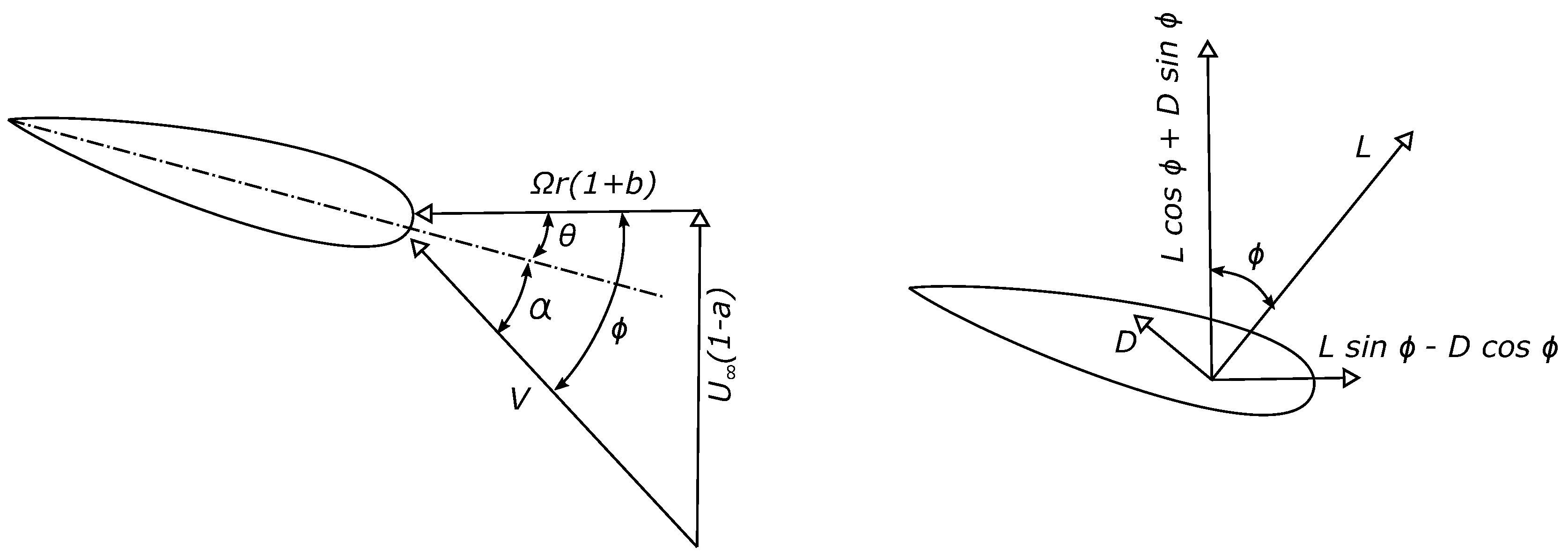
2.1.2. Blade Element Theory

The blade element theory divides the rotor blade into several discrete radial elements (airfoils) as described earlier in Section 2.1. This theory relies on two key assumptions: (1) There are no aerodynamic interactions between the 2D airfoil elements in different sections, and (2) the forces acting on the elements are solely determined by the lift and drag characteristics of the airfoils shape and relative inflow [1].

The definitions of the velocity vector and the lift (L) and drag (D) acting on the blade section are illustrated in Figure 2. The total angle between the circumferential direction to the relative inflow (V) is represented by variable $\varphi$. This angle is composed by the local angle of attack ($\alpha$) and the sum of the pitch and twist angles ($\theta$). The variable $U_{\infty }$ represents the inflow wind speed and $\Omega$ is the rotational speed of the turbine. Please note that $U_{\infty }$ in Figure 2 is the same as U used in Section 2.1.1.

The axial force and torque acting on the blade element can be obtained using the relations for lift and drag, that are represented by the lift ($C_L$) and drag ($C_D$) coefficients assuming the chord length (c) of the blade element is known from the geometrical model. These are formulated as following

$$d{F}_A=N\frac{1}{2}\rho V^{2}c(C_L\cos \varphi +C_D\sin \varphi )dr$$

(10)

$$dT=N\frac{1}{2}\rho V^{2}cr(C_L\sin \varphi -C_D\cos \varphi )dr.$$

(11)

By introducing a new parameter that represents the ratio of the tangential to the inflow velocity, ${\lambda }_r=\frac{r\Omega }{U_{\infty }}$, well known as the local speed ratio, the total flow angle can be redefined as

$$\varphi ={\tan }^{-1}\left(\frac{U(1-a)}{r\Omega (1+b)}\right)={\tan }^{-1}\left(\frac{(1-a)}{{\lambda }_r(1+b)}\right).$$

(12)

2.1.3. B-GO Code Description

A short description of the BEM code B-GO will be presented in the following section. The B-GO code was written in Python language employing several commonly used packages. B-GO is constructed by several subroutines that is called in the main calculations. These routines are read_data, variable_assignment, data_preparation, interpolate_polar, interpolate_radial, extrapolation, induction_calculation and tip_loss_correction, illustrated in Figure 3. By writing each main part of the code as a subroutine, the code can be further developed in the future by simply modifying only the respective functions.

The BEM computation is started by reading the input data. First, the axial (a) and tangential ($a^{\prime }$) induction factors are set to a small value (0.0001) to initialize the calculation. The angle of attack is calculated by applying the following formula

$$\alpha =\varphi -\theta .$$

(13)

$C_L$ and $C_D$ can then be obtained from the polar data of the respective sections. Please note that interpolation and extrapolation of the polar data are necessary because there is a high probability that the polar data does not exist for the corresponding angle of attack. The interpolation can be carried out using one of the three different interpolation options that the user can choose, namely linear-, quadratic- and cubic-spline interpolations. These can be expressed as:

$$S_{1,n}\left(x\right)=\left\{\begin{array}{cc}{p}_1\left(x\right)=f_0\frac{x-x_1}{x_0-x_1}+f_1\frac{x-x_0}{x_1-x_0}\hfill & x\in [x_0,x_1]\hfill \\ p_2\left(x\right)=f_1\frac{x-x_2}{x_1-x_2}+f_2\frac{x-x_1}{x_2-x_1}\hfill & x\in [x_1,x_2]\hfill \\ ⋮\hfill \\ p_n\left(x\right)=f_{n-1}\frac{x-x_n}{x_{n-1}-x_n}+f_n\frac{x-x_{n-1}}{x_n-x_{n-1}}\hfill & x\in [x_{n-1},x_n]\hfill \end{array}\right.$$

(14)

$$S_{2,n}\left(x\right)=\left\{\begin{array}{cc}{p}_1\left(x\right)=a_1+b_{1}x+c_1{x}^2\hfill & x\in [x_0,x_1]\hfill \\ p_2\left(x\right)=a_2+b_{2}x+c_2{x}^2\hfill & x\in [x_1,x_2]\hfill \\ ⋮\hfill \\ p_n\left(x\right)=a_n+b_{n}x+c_n{x}^2\hfill & x\in [x_{n-1},x_n]\hfill \end{array}\right.$$

(15)

$$S_{3,n}\left(x\right)=\left\{\begin{array}{cc}{p}_1\left(x\right)=a_1+b_{1}x+c_1{x}^2+d_1{x}^3\hfill & x\in [x_0,x_1]\hfill \\ p_2\left(x\right)=a_2+b_{2}x+c_2{x}^2+d_2{x}^3\hfill & x\in [x_1,x_2]\hfill \\ ⋮\hfill \\ p_n\left(x\right)=a_n+b_{n}x+c_n{x}^2+d_n{x}^3\hfill & x\in [x_{n-1},x_n]\hfill \end{array}\right.$$

(16)

where $S_{1,n}\left(x\right)$, $S_{2,n}\left(x\right)$ and $S_{3,n}\left(x\right)$ are the linear, quadratic and cubic continuous functions, respectively, that interpolate the data constructed by several polynomials $p_1\left(x\right)$, $p_1\left(x\right)$, ..., $p_n\left(x\right)$. The constants ($a_n$, $b_n$, $c_n$, $d_n$) shall be determined on each function for the corresponding dataset range $[x_{n-1},x_n]$. Most of BEM codes usually employ the linear interpolation approach. New a and $a^{\prime }$ can be calculated using

$$a=\frac{1}{\phantom{(}\frac{4}{\phantom{(}{C}_n\sigma }{F}_{tip}{\sin }^2\varphi +1}$$

(17)

$$a^{\prime }=\frac{1}{\phantom{(}\frac{4}{\phantom{(}{C}_t\sigma }{F}_{tip}\sin \varphi \cos \varphi -1},$$

(18)

where

$$C_n=C_L\cos \varphi +C_D\sin \varphi$$

(19)

$$C_t=C_L\sin \varphi -C_D\cos \varphi$$

(20)

$$\sigma =\frac{cB}{2\pi r}.$$

(21)

The Prandtl tip loss correction is given as [8]

$$F_{tip}=\frac{2}{\pi }{\cos }^{-1}\left(e^{-\frac{B(R-r)\sqrt{1+{\lambda }^2}}{\phantom{(}2R}}\right),$$

(22)

where B and R are the number of blades and the rotor radius, respectively. The obtained inductions are then compared with the inductions from the previous iteration, and the residual is calculated. The converge is defined when the residual is smaller than the user defined tolerance, that was set to 1 × 10${}^{-11}$ for the present studies. Otherwise, 100 iterations were applied. The calculations are performed for each blade section until the maximum number of blade elements of N. The interpolation is also applied to refine the evaluated segments in the radial directions, both for the polar and the blade geometry, using one of the three available interpolation options as mentioned above. This allows a more accurate computation to be performed.

In case the induction factor is higher than 0.4, the Froude momentum theory is no longer valid. Spera [37] suggested a correction for the axial induction, if $a>a_c$, as

$$a=1+\frac{1}{2}K(1-2a_c)-\frac{1}{2}\sqrt{{(K(1-2a_c)+2)}^2+4(K{a}_c^2-1)}$$

(23)

where $a_c$ is commonly about 0.2 and K is defined as

$$K=\frac{4F_{tip}{\sin }^2\varphi }{\sigma C_n}.$$

(24)

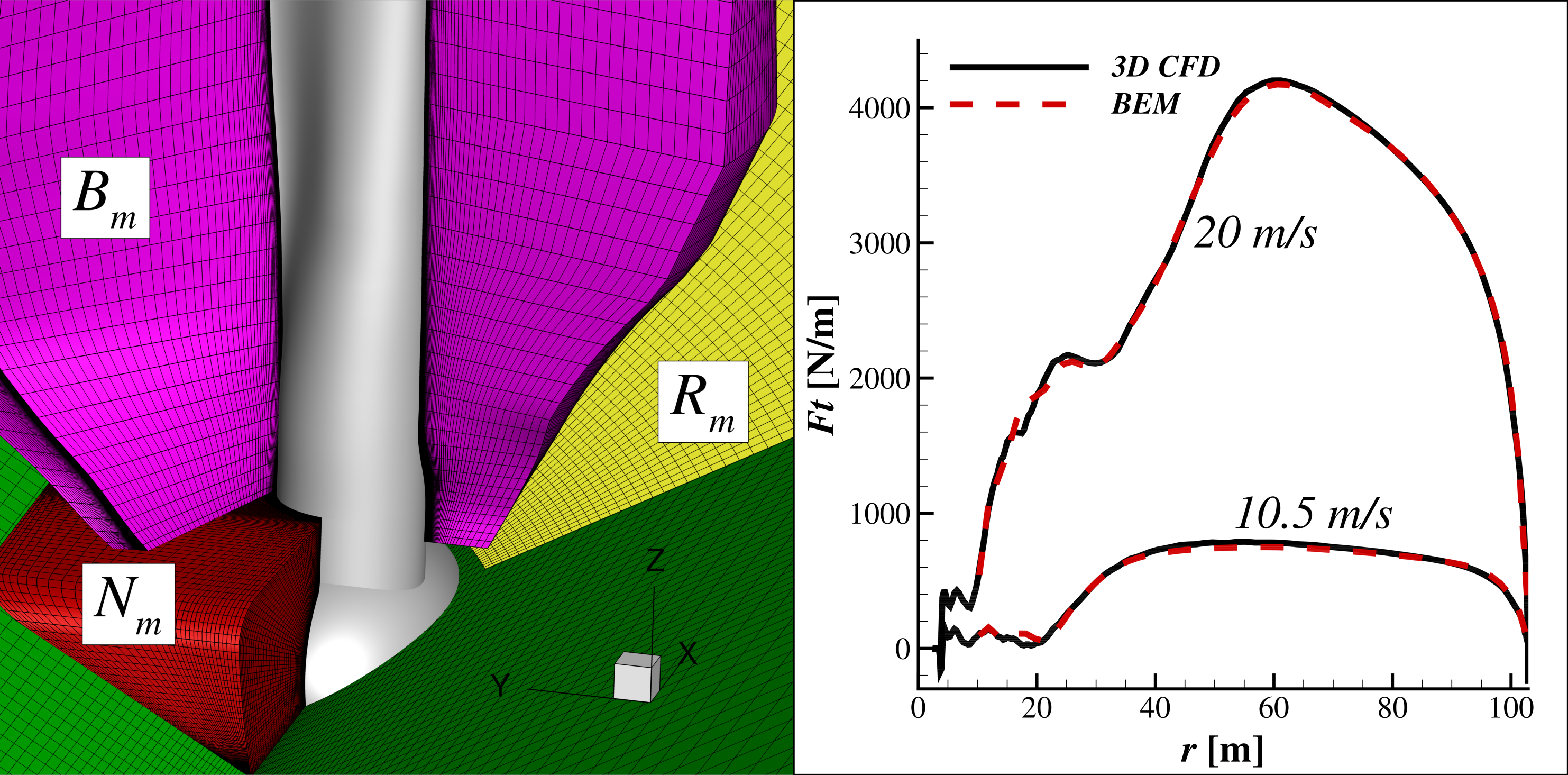
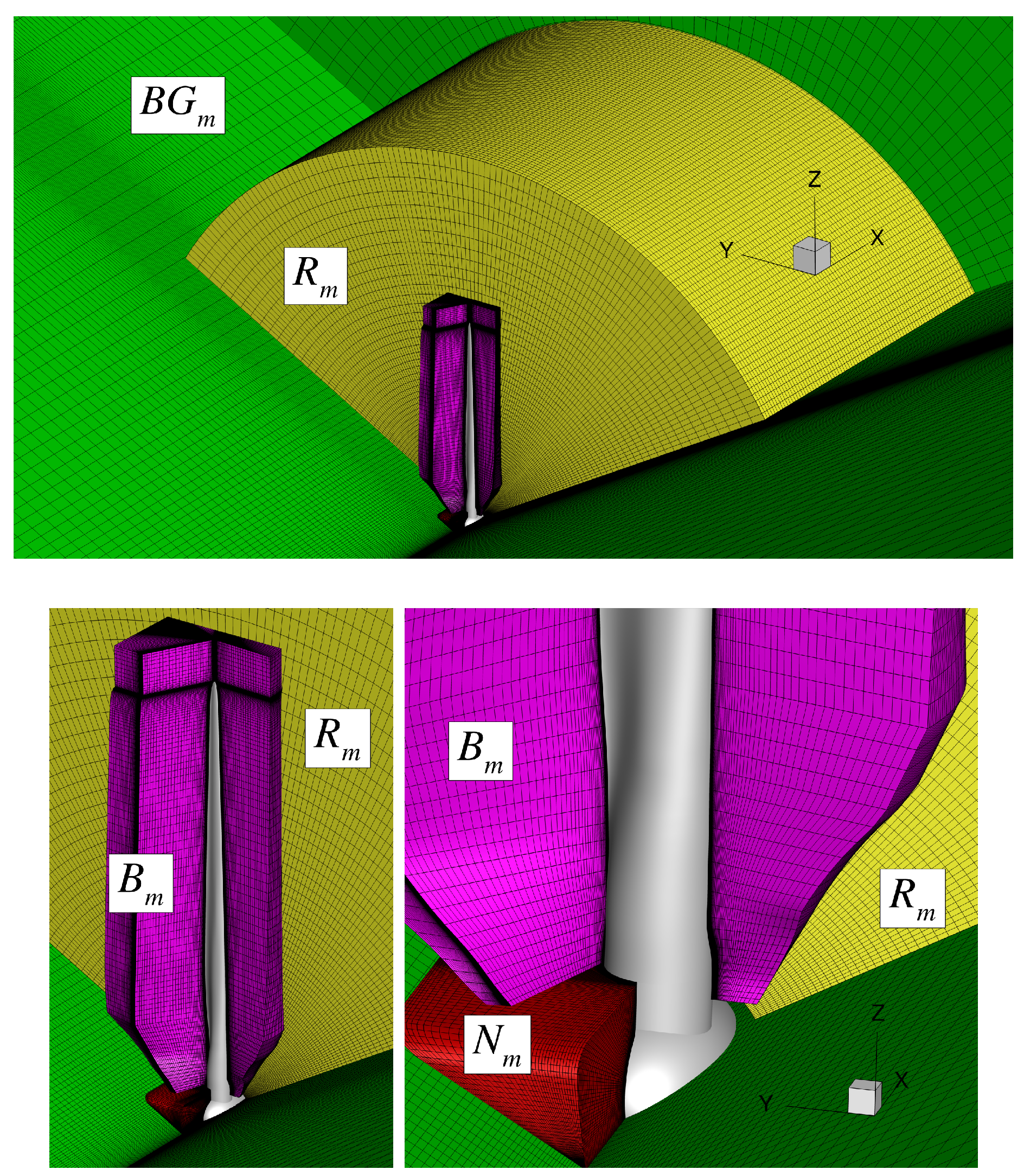
2.2. Computational Fluid Dynamics

The Computational Fluid Dynamics (CFD) approach is a combination of interdisciplinary fields such as physics, numerical mathematics and computer sciences to model the physical fluid flow phenomena. Turbulence is the main concern for accuracy and applicability for flow simulations using CFD. One way out of this issue is to simplify the solution variables of the Navier-Stokes equations by the Reynolds-Averaged Navier-Stokes (RANS) approach, which pose the time-averaged form of the Navier-Stokes equations. The fluid flow variables in the governing equations are subdivided into the mean and fluctuating components. For compressible flow, it is advocated to use the weighted density well known as the Favré averaging technique. This is done by using the Reynolds averaging for density and pressure, yet for velocity, internal energy, enthalpy and temperature the Favré averaging procedure can be used [38,39,40]. The Favré averaged equation for velocity is acquired using:

$$\begin{array}{c}\hfill {\tilde{u}}_i=\frac{1}{\overline{\rho }}\underset{T\to \infty }{lim}\frac{1}{T}{\int }_t^{t+T}\rho u_i\mathrm{ṭ}.\end{array}$$

(25)

The Favré decomposition can be also written as $u_i={\tilde{u}}_i+u_i^{″}$. The Reynolds-averaged density is embodied by $\overline{\rho }$, the mean velocity is symbolized by $\widetilde{u_i}$, and $u_i^{″}$ stands for the fluctuating part of the velocity accordingly [38]. The average of the fluctuating part is zero. For correlated quantities, the averaged product of the two fluctuating quantities is not zero. If the Reynolds averaging is employed for density and pressure and the Favré averaging to the other flow variables, the average momentum equation is obtained. This mathematical expression is referred to as the Favré- and Reynolds-averaged Navier-Stokes equations [13]. In the cartesian tensor form the equations add up to

$$\begin{array}{c}\frac{\partial \overline{\rho }}{\partial t}+\frac{\partial }{\partial x_i}\left(\overline{\rho }{\tilde{u}}_i\right)=0\end{array}$$

(26)

$$\begin{array}{c}\frac{\partial }{\partial t}\left(\overline{\rho }{\tilde{u}}_i\right)+\frac{\partial }{\partial x_j}\left(\overline{\rho }{\tilde{u}}_i{\tilde{u}}_j\right)=\frac{\partial \overline{p}}{\partial x_i}+\frac{\partial }{\partial x_j}\left[\mu \left(\frac{\partial {\tilde{u}}_i}{\partial x_j}+\frac{\partial {\tilde{u}}_j}{\partial x_i}\right)\right]-\frac{\partial }{\partial x_j}{\tilde{\tau }}_{ij}^{\mathrm{RANS}}.\end{array}$$

(27)

The left hand side of Equation (27) accounts for the fluid momentum incorporating the variation of the mean flow with the time. This is balanced by the mean pressure gradient, viscous stresses and the apparent stress ${\tilde{\tau }}_{ij}^{\mathrm{RANS}}$, also known as the Reynolds stress (Favré-averaged) on the other side of the equation. Since the equation cannot directly be solved, the equation is remodeled to close the equation [13]. The Boussinesq hypothesis is generally taken as an approach to relate the mean velocity gradients to the Reynolds stress, for comparison see Hinze [41]. In this model the turbulent viscosity is expressed in the variable ${\mu }_t$ [13].

$$\begin{array}{c}\hfill -{\tilde{\tau }}_{ij}^{\mathrm{RANS}}={\mu }_t\left(\frac{\partial {\tilde{u}}_i}{\partial x_j}+\frac{\partial {\tilde{u}}_j}{\partial x_i}\right)-\frac{2}{3}\left(\overline{p}\tilde{k}+{\mu }_t\frac{\partial {\tilde{u}}_k}{\partial x_k}\right){\delta }_{ij}\end{array}$$

(28)

Many turbulence models are developed based on this relation through the modeling of the turbulent viscosity, commonly referred to as eddy viscosity turbulence models (EVTMs). Examples of the EVTMs are the Spalart-Allmaras (SA) model and its derivatives (1-equation), $k-\epsilon$ model and the $k-\omega$ model and their derivatives (2-equation), and the Reynolds stress model (RSM) and its derivatives (7-equation). The shear stress transport (SST) $k-\omega$ model according to Menter [21] is a two-equation model family widely used in industry and research, because the model is able to deliver reasonable predictions for flows with a strong adverse pressure gradient. The model can be mathematically expressed as

$$\begin{array}{c}\frac{\partial \rho k}{\partial t}+\frac{\partial \rho u_{j}k}{\partial x_j}=P-{\beta }^{*}\rho \omega k+\frac{\partial }{\partial x_j}\left[\left(\mu +{\sigma }_k{\mu }_t\right)\frac{\partial k}{\partial x_j}\right]\end{array}$$

(29)

$$\begin{array}{c}\frac{\partial \rho \omega }{\partial t}+\frac{\partial \rho u_j\omega }{\partial x_j}=\frac{\gamma \omega }{{\nu }_t}P-\beta \rho {\omega }^2+\frac{\partial }{\partial x_j}\left[\left(\mu +{\sigma }_{\omega }{\mu }_t\right)\frac{\partial \omega }{\partial x_j}\right]+2\left(1-F_1\right)\frac{\rho {\sigma }_{{\omega }_2}}{\omega }\frac{\partial k}{\partial x_j}\frac{\partial \omega }{\partial x_j}.\end{array}$$

(30)

The parameters used in these equations are determined as

$$\begin{array}{c}P={\tau }_{ij}\frac{u_i}{x_j}\end{array}$$

(31)

$$\begin{array}{c}{\tau }_{ij}={\mu }_t\left(2S_{ij}-\frac{2}{3}\rho k{\delta }_{ij}\right)\end{array}$$

(32)

$$\begin{array}{c}{S}_{ij}=\frac{1}{2}\left(\frac{u_i}{x_j}+\frac{u_j}{x_i}\right)\end{array}$$

(33)

$$\begin{array}{c}{\mu }_t=\frac{\rho a_{1}k}{max\left(a_1\omega ,\Omega F_2\right)}.\end{array}$$

(34)

For the present studies, the generic 10 MW AVATAR blade [42] was chosen. The rotor is designed based on the DTU 10 MW wind turbine [43] with a larger blade radius of R = 102.9 m. The blade was constructed by 6 different DU airfoils as presented in

Table 1. Airfoil sections used for the AVATAR reference blade [15,42].

Airfoil Thickness [$\mathit{t}/\mathit{c}$]	Airfoil Type
60.0%	Artificial, based on thickest available DU
40.1%	DU 00-W2-401
35.0%	DU 00-W2-350
30.0%	DU 97-W300
24.0%	DU 91-W2-250 (modified for $t/c=$ 24%)
21.0%	Based on DU 00-W212, added trailing edge thickness

. The airfoils are interpolated along the blade radius, and the shapes are illustrated in Figure 4. For further detail, the reader is suggested to refer to [42]. The calculations were performed without tower to avoid the unsteady tower disturbance effects. A Cartesian coordinate system was adopted in the present studies, where the details are illustrated in Figure 5. In the rotating (local) coordinate system, x, y and z represent chordwise, normal and spanwise directions of the blade which rotate together with the rotor.

The grid for the rotor simulations consist of several components, background ($B{G}_m$), wake refinement ($R_m$), blade ($B_m$) and nacelle ($N_m$) meshes as shown in Figure 6. The blade mesh consists of 280 × 128 cells in chordwise and normal directions, respectively. The blade is discretized by 192 cells along the radius with significant refinement near the root and tip areas. Figure 5 shows the surface meshes and the sectional mesh of the blade used in the present investigations. The mesh of the blade is C-H type and was constructed using the commercial grid generator Gridgen [44] with the “automesh” script developed at the institute. The 3D blade mesh was refined near the wall area satisfying the non-dimensional wall distance $y^{+}<$ 1 to resolve the viscous sub-layer. The total resolution for the complete domain reaches 39 million grid points.

The CFD FLOWer code [45,46] was used to numerically model the fluid flow over the rotor by solving the Navier-Stokes equations on the structured meshes. A central scheme based on the Jameson-Schmidt-Turkel (JST) formulation was employed for flux discretization, resulting in a second order accuracy on smooth meshes. For turbulent closure, the two-equation shear stress transport (SST) $k-\omega$ model according to Menter [21] was used. In the present analysis, fully turbulent computations were carried out for the 3D rotor. The simulations were performed with the time step size of 0.037 s which corresponds to two degree blade revolution per physical time step. The time step can be calculated as $\Delta t\left[s\right]=\Delta t{[}^{\circ }]/(\Omega {360}^{\circ })$, where $\Delta t{[}^{\circ }]$ is the azimuthal time step size. Each physical time step was iterated towards a pseudo steady state using 35 sub-iterations. The simulations have been carried out for 11 rotor revolutions. The last one revolution was employed for the data extraction purpose. The impacts of different rotor revolutions on the extracted data are shown in [13]. The basic sensitivity of the CFD computations towards the blade grid and time resolutions have been presented in Ref [15,47], respectively. For a better overview of the grid convergence studies, the results of the quantified grid convergence index (GCI) according to Celik et al. [48] are presented in

Table 2. Grid convergence study for the AVATAR blade using the GCI approach. Data are obtained from the URANS calculations.

Parameter	Power	Thrust
Value fine	9.28 × 10${}^6$ W	1.330 × 10${}^6$ N
Value medium	9.26 × 10${}^6$ W	1.328 × 10${}^6$ N
Value coarse	9.20 × 10${}^6$ W	1.326 × 10${}^6$ N
Extrapolated rel. error
-fine	0.12%	0.27%
-medium	0.36%	0.47%
-coarse	1.02%	0.58%
Grid convercence index	0.15%	0.34%

and the sectional loads are shown in Figure 7. The coarse blade mesh consists of 136 cells in radial direction (blade total cells number of 8.1 × 10${}^6$), medium mesh of 192 cells (10.9 × 10${}^6$) and fine mesh of 272 cells (15.9 × 10${}^6$). The background, wake refinement and nacelle meshes consist of 1.9 × 10${}^6$, 16.34 × 10${}^6$ and 3.5 × 10${}^6$ cells, respectively. The grid convergence index for the fine grid is very small (less than 0.5%), stating that the solutions are spatially converged. It can be seen that the magnitude of power and thrust for the medium and the fine grids are very close. The extrapolated relative errors are less than 0.5% in both parameters, while a higher error is observed for the coarse grid due to inaccurate prediction of the sectional forces in the blade inboard region. This is indicated in the sectional loads predictions displayed in Figure 7 showing the sectional axial ($F_n$) and tangential force ($F_t$) distributions over the radius. It can be seen clearly that the coarse grid shows a strong underestimation of the sectional loads in the inboard area at $r\approx$ 20 m. The main reason is that the rotational augmentation effects are not well captured by the corresponding grid, that separated flow is stronger. On the other hand, the medium and fine grids have similar results, indicating grid convergence. Considering the accuracy and computational effort, the selection of the medium grid for CFD simulations is reasonable.

3. Results and Discussion

3.1. 3D CFD and BEM Comparison

This section presents the results of the comparative studies between the expensive fully resolved CFD with the lower fidelity BEM computations for the AVATAR turbine. The simulations were conducted at a wind speed of $U_{\infty }$ = 10.5 m/s, rotational speed of n = 9.02 rpm and at zero pitch angle (${\alpha }_p$). This is the standard test case in the code-to-code comparison for the AVATAR project in [24]. To avoid the necessity for 3D correction in the root area, the 3D polar data extracted from CFD simulations in Ref [15] were considered in the BEM computations. The term 3D polar means that the polar data is obtained directly from the 3D CFD simulations of wind turbine. In this sense, all the 3D effects are already included in the polar. To demonstrate that this polar dataset is suitable for the computations, two different polar datasets, namely the polar obtained from 2D CFD computations with and without a stall delay model based on [49], are considered for comparison. The same 2D polar datasets were used in [50]. The comparison is displayed in Figure 8, showing $F_n$ $F_t$ distributions over the blade radius. Please note that the Prandtl tip loss correction is activated only for the 2D polar data, with and without the stall delay model. It is clearly shown that the 3D CFD simulations can only be modelled accurately by the use of the 3D polar dataset, especially in the root area. The pure 2D polar definitely underestimates the loads in the inboard region of the blade as the 3D rotational effect is missing. The use of the stall delay model improves the BEM prediction at certain regions. However, the blade forces are overestimated significantly in the extreme root area for $r\le$ 20 m. A slight overestimation is also observed starting for $r\le$ 40 m for $F_n$. The quantified error of the BEM simulations relative to the 3D CFD results is presented in

Table 3. Error quantification of the sectional loads with respect to the 3D CFD data.

	$\mathit{ϵ}$$\mathit{Fn}$ [%]			$\mathit{ϵ}$$\mathit{Ft}$ [%]
	r = 15 m	r = 60 m	r = 90 m	r = 15 m	r = 60 m	r = 90 m
2D Polar	99.01	3.45	2.56	598.24	6.67	6.06
2D Polar + Stall Delay	127.80	3.19	2.56	468.88	6.48	6.06
3D Polar	11.84	3.08	0.24	19.58	4.81	0.33

. In Figure 9, the effects of the polar origin on the $C_L$, $C_D$ and $\alpha$ distributions are presented. A large discrepancy between the results is observed in the grey shaded area in the root region of the blade in comparison with the 3D CFD results when the 2D polar is employed. The uncorrected 2D polar underestimates $C_L$ while the corrected 2D polar overestimates it. It is interesting to see that an inverse behaviour is shown for $\alpha$. In terms of $C_D$, results from the 2D and 2D corrected polars consistently show overpredictive values within this area. In contrast, the usage of the 3D polar extracted from the 3D CFD simulations yields a consistent agreement with the 3D CFD data.

Despite the usefulness of the 3D polar, there is a limitation of its use. For example, it requires the expensive 3D simulations to be carried out in advance and the tip loss effect is already present in the extracted polar results. Regarding the latter, it is an advantage for BEM because this removes the dependency of the calculations on the employed tip loss model, but is a side effect when a lifting line approach will be used as the tip loss is calculated directly in the calculation of the induced velocity itself. Therefore, a simple approach combining the 3D polar dataset with the 2D polar is suggested in the present studies. The 2D polar, for example, can be applied in the region that is affected by the tip loss influence. This is expected to arise starting from $r\ge$ 90 m. The evidence of this can be seen on the $\alpha$ and $C_L$ distributions in Figure 10, indicated by the vertical lines. Figure 11 displays the comparison of three cases; (1) 3D polar without a tip loss, (2) 3D polar with a tip loss model and (3) hybrid polar with a tip loss model. It is shown that the 3D polar dataset accuracy in modelling the axial (Figure 11a) and tangential (Figure 11b) forces near the tip area reduces as the tip loss model is activated. The use of the hybrid polar is clearly able to minimize this drawback. Despite that, the hybrid polar trend is clearly different than the 3D CFD results in terms of the induction distributions. Figure 11c shows the axial induction (a) distributions predicted using different models. It can be seen that the pure 3D and the hybrid polar datasets predict an increasing axial induction factor near the tip when the tip loss model is activated. This is caused simply by the modelling behaviour of the Prandtl tip loss factor that increases the induction term in order to reduce the local effective angle of attack. A similar behaviour is observed for the tangential induction ($a^{\prime }$) distribution shown in Figure 11d, but is less prominent. The local drop and increase of the tangential induction in the middle and in the root area is hardly captured by BEM using all polar datasets. This fluctuating behaviour is caused by the trailing vortices influence within that area as demonstrated in [13,47], that surely cannot be modelled by BEM.

As the polar and the blade geometry has to be interpolated, the use of several interpolation options in B-GO for BEM predictions is investigated. Figure 12 presents the influence of the linear and cubic spline interpolations for polar on the BEM results. It can be seen that the effect of polar interpolation is minimum if the polar data points for a blade section is sufficient. Experience has shown that if the data points are limited, i.e., the polar has no enough resolution, the interpolation option can determine the accuracy of the results.

The interpolation order of the blade geometry and the polar in radial direction, however, can strongly influence the results as demonstrated in Figure 13, Figure 14, Figure 15 and Figure 16. For linear interpolation in Figure 13, it can be seen that the number of blade elements strongly influence the accuracy of the prediction especially in the tip area of the blade. With increasing blade element number, the accuracy of the computation improves. This is, however, does not hold true for the quadratic interpolation displayed in Figure 14. A prominent periodic change of the polar trend is shown in the middle part of the blade even though though the accuracy of the results near the tip improves. Therefore, this interpolation type is not recommended for further simulations. Figure 15 shows the effects of using the cubic interpolation approach on the results. It can be seen that the accuracy improves significantly for all blade regions by increasing the blade elements from 10 to 20. This interpolation type shows a better prediction than the linear interpolation for the same amount of blade elements. This behaviour is shown in Figure 16 where the BEM prediction using the cubic interpolation is more accurate than the linear interpolation especially at the maximum axial force level in Figure 16a. Therefore, the cubic interpolation is suggested for further studies.

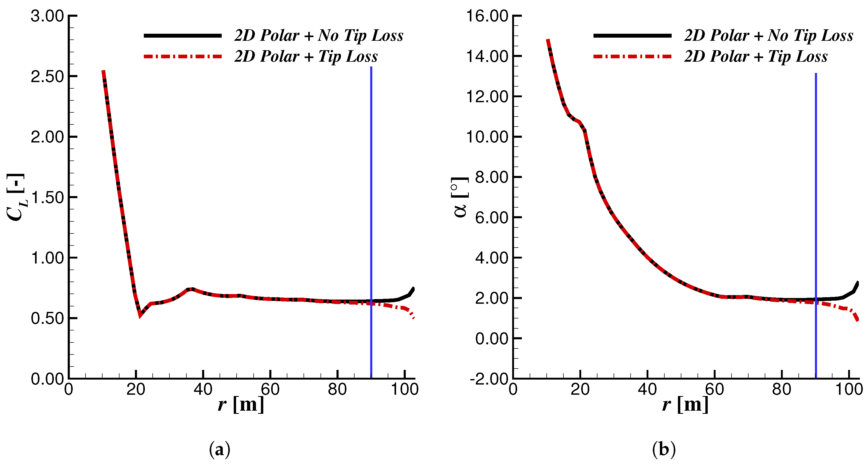
3.2. Simulations at Various Operating Conditions

In this sections, the influence of various operating conditions on the rotor performance is evaluated. Figure 17 presents the numerical simulations of the AVATAR rotor for two different wind speeds, namely $U_{\infty }$ = 10.5 m/s and 20 m/s. The rotational speed and pitch angle are kept constant (n = 9.02 rpm and ${\alpha }_p$ = 0${}^{\circ }$). The higher wind speed case is characterized by massive flow separation for most of the blade sections as the operating angle of attack is high, especially in the inboard area as already shown in [47]. Despite that, the BEM simulations carried out in the B-GO code are able to mimic the 3D CFD results with an excellent agreement for the whole blade region. This indicates that the use of the 3D polar data and cubic interpolation for polar and blade geometry is a suitable approach to be used for wind turbine simulations at various flow situations.

In Figure 18, the effects of tip speed ratio ($\lambda$) and pitch angle of the blade on the rotor performance are evaluated. The results of the 3D CFD simulations are also presented for comparison. Three different pitch angles are considered; ${\alpha }_p$ = −5${}^{\circ }$, 0${}^{\circ }$ and 5${}^{\circ }$. Please note that positive pitch reduces the angle of attack. It can be seen that the turbine power coefficient $C_P$ is about 0.2 regardless of the pitch angle value. This shows that a higher pitch angle than 5${}^{\circ }$ is required to control the turbine when it is operating at a wind speed higher than 20 m/s, assuming the rotational speed is 9.02 rpm. With increasing $\lambda$, the power coefficient value differs considerably. The smallest pitch angle generates the most mechanical power as the angle of attack increases. The operating range of the turbine is also broader, from 2 $<\lambda <$ 14, that is ideal for the turbine operation. The turbine performance in terms of the power coefficient reduces accordingly as the pitch angle increases to 0${}^{\circ }$ and 5${}^{\circ }$. The maximum power coefficient is, however, located at a similar flow situation for ${\alpha }_p$ = −5${}^{\circ }$ and 0${}^{\circ }$ at $\lambda \approx$ 9, while it occurs at $\lambda \approx$ 5.5 for ${\alpha }_p$ = 5${}^{\circ }$. Despite that, the increased power coefficient for the reduced pitch angle is not appearing without price. The thrust coefficient $C_T$ increases considerably for the lower pitch value than the higher one. This may be dangerous for the rotor and tower structure and may reduce the lifetime of the machines.

4. Conclusions

Numerical simulations employing Blade Element and Momentum (BEM) and Computational Fluid Dynamics (CFD) approaches for a large 10 MW wind turbine have been carried out. The AVATAR (Advanced Aerodynamic Tools for Large Rotors) turbine with a diameter of 205.8 m developed within the framework of the AVATAR project was chosen for this purpose.

A careful selection of the polar dataset for BEM computations is important to ensure the accuracy of the results. It was shown that the 3D polar obtained from fully resolved 3D CFD simulations is the most accurate dataset. The inability of the 3D polar to use the tip loss correction in BEM or ultimately in the lifting line approach can be compensated by using the hybrid polar, replacing the area where the tip loss appear by the 2D polar data. The accuracy of the BEM computations is also influenced by the discretization of the blade segments and how they are interpolated from the existing polar dataset. The studies reveal that the cubic-spline interpolation is suitable for the prediction. The linear interpolation is also suitable for this purpose. However, it requires more number of blade segments to achieve similar results especially in the tip area. On the other hand, the quadratic-spline interpolation produces non physical oscillations of the data in the middle blade area. Thus, this is not recommended to be used for later studies. Considering all the parameters above, the comparison between BEM and CFD shows an excellent agreement for all blade sections even at a high wind speed case where massive flow separation takes place in the inboard area. At last, it has been documented that the turbine performance depends upon the pitch angle and tip speed ratio. The smaller pitch angle increases the maximum power coefficient and rotor operating range, but the thrust force coefficient enhances as well as a price. This may put more stress on the structure and can reduce the lifetime of the machine itself.

References

1. Bangga, G.; Hutomo, G.; Syawitri, T.; Kusumadewi, T.; Oktavia, W.; Sabila, A.; Setiadi, H.; Faisal, M.; Hendranata, Y.; Lastomo, D.; et al. Enhancing BEM simulations of a stalled wind turbine using a 3D correction model. J. Phys. Conf. Ser. 2018, 974, 012020. [Google Scholar] [CrossRef] [Green Version]
2. Hutomo, G.; Bangga, G.; Sasongko, H. CFD studies of the dynamic stall characteristics on a rotating airfoil. Appl. Mech. Mater. 2016, 836, 109–114. [Google Scholar] [CrossRef]
3. Bangga, G.; Lutz, T.; Dessoky, A.; Krämer, E. Unsteady Navier-Stokes studies on loads, wake, and dynamic stall characteristics of a two-bladed vertical axis wind turbine. J. Renew. Sustain. Energy 2017, 9, 053303. [Google Scholar] [CrossRef] [Green Version]
4. Betz, A. Das Maximum der theoretisch möglichen Ausnutzung des Windes durch Windmotoren. Zeitschrift Gesamte Turbinenwesten 1920, 20, 307–309. [Google Scholar]
5. Gasch, R.; Twele, J. Wind Power Plants: Fundamentals, Design, Construction and Operation; Springer Science & Business Media: Berlin, Germany, 2011. [Google Scholar]
6. Glauert, H. The Elements of Aerofoil and Airscrew Theory; Cambridge University Press: Cambridge, UK, 1983. [Google Scholar]
7. Ingram, G. Wind Turbine Blade Analysis Using the Blade Element Momentum Method Version 1.0; School of Engineering, Durham University: Durham, UK, 2005. [Google Scholar]
8. Prandtl, L.; Betz, A. Vier Abhandlungen zur Hydrodynamik und Aerodynamik; Universitätsverlag Göttingen: Göttingen, Germany, 2010; Volume 3. [Google Scholar]
9. Himmelskamp, H. Profile Investigations on a Rotating Airscrew; MAP: Göttingen, Germany, 1947. [Google Scholar]
10. Sørensen, J.N. Three-Level, Viscous-Inviscid Interaction Technique for the Prediction of Separated Flow Past Rotating Wing. Ph.D. Thesis, Technical University of Denmark (DTU), Lyngby, Denmark, 1986. [Google Scholar]
11. Snel, H.; Houwink, R.; Bosschers, J.; Piers, W.; Van Bussel, G.; Bruining, A. Sectional prediction of 3D effects for stalled flow on rotating blades and comparison with measurements. In Proceedings of the European Community Wind Energy Conference, HS Stevens and Associates, LÃ1, Travemuende, Germany, 8–12 March 1993; Volume 4. [Google Scholar]
12. Du, Z.; Selig, M. The effect of rotation on the boundary layer of a wind turbine blade. Renew. Energy 2000, 20, 167–181. [Google Scholar] [CrossRef]
13. Bangga, G. Three-Dimensional Flow in the Root Region of Wind Turbine Rotors; Kassel University Press GmbH: Kassel, Germany, 2018. [Google Scholar]
14. Bangga, G.; Kim, Y.; Lutz, T.; Weihing, P.; Krämer, E. Investigations of the inflow turbulence effect on rotational augmentation by means of CFD. J. Phys. Conf. Ser. 2016, 753, 022026. [Google Scholar] [CrossRef]
15. Bangga, G.; Lutz, T.; Jost, E.; Krämer, E. CFD studies on rotational augmentation at the inboard sections of a 10 MW wind turbine rotor. J. Renew. Sustain. Energy 2017, 9, 023304. [Google Scholar] [CrossRef]
16. Bangga, G.; Lutz, T.; Krämer, E. Root flow characteristics and 3D effects of an isolated wind turbine rotor. J. Mech. Sci. Technol. 2017, 31, 3839–3844. [Google Scholar] [CrossRef]
17. Wood, D. A three-dimensional analysis of stall-delay on a horizontal-axis wind turbine. J. Wind Eng. Ind. Aerodyn. 1991, 37, 1–14. [Google Scholar] [CrossRef]
18. Duque, E.P.; Burklund, M.D.; Johnson, W. Navier-Stokes and comprehensive analysis performance predictions of the NREL phase VI experiment. In Proceedings of the Wind Energy Symposium, Reno, NV, USA, 6–9 January 2003; pp. 43–61. [Google Scholar]
19. Pape, A.L.; Lecanu, J. 3D Navier–Stokes computations of a stall-regulated wind turbine. Wind Energy Int. J. Prog. Appl. Wind Power Convers. Technol. 2004, 7, 309–324. [Google Scholar] [CrossRef]
20. Wilcox, D.C. Turbulence Modeling for CFD; DCW Industries: La Cañada Flintridge, CA, USA, 1998; Volume 2. [Google Scholar]
21. Menter, F.R. Two-equation eddy-viscosity turbulence models for engineering applications. AIAA J. 1994, 32, 1598–1605. [Google Scholar] [CrossRef] [Green Version]
22. Bangga, G.; Weihing, P.; Lutz, T.; Krämer, E. Effect of computational grid on accurate prediction of a wind turbine rotor using delayed detached-eddy simulations. J. Mech. Sci. Technol. 2017, 31, 2359–2364. [Google Scholar] [CrossRef]
23. Boorsma, K.; Schepers, J. New MEXICO experiment. Preliminary Overview with Initial Validation Technical Report ECN-E–14-048 ECN. 2014. Available online: https://www.ecn.nl/docs/library/report/2014/e14048.pdf (accessed on 16 October 2018).
24. Sørensen, N.; Hansen, N.; Garcia, N.; Florentie, L.; Boorsma, K.; Gomez-Iradi, S.; Prospathopoulus, J.; Barakos, G.; Wang, Y.; Jost, E.; et al. AVATAR D2. 3–Power Curve Predictions. AVATAR Proj. 2015. Available online: http://www.eera-avatar.eu/fileadmin/mexnext/user/report-d2p3.pdf (accessed on 16 October 2018).
25. Schneider, M.S.; Nitzsche, J.; Hennings, H. Accurate load prediction by BEM with airfoil data from 3D RANS simulations. J. Phys. Conf. Ser. 2016, 753, 082016. [Google Scholar] [CrossRef] [Green Version]
26. Guma, G.; Bangga, G.; Jost, E.; Lutz, T.; Krämer, E. Consistent 3D CFD and BEM simulations of a research turbine considering rotational augmentation. J. Phys. Conf. Ser. 2018, 1037, 022024. [Google Scholar] [CrossRef]
27. Jonkman, J.M.; Buhl, M.L., Jr. FAST User’S Guide; Technical Report No. NREL/EL-500-38230; National Renewable Energy Laboratory: Golden, CO, USA, 2005.
28. Marten, D.; Wendler, J.; Pechlivanoglou, G.; Nayeri, C.; Paschereit, C. QBLADE: An open source tool for design and simulation of horizontal and vertical axis wind turbines. Int. J. Emerg. Technol. Adv. Eng. 2013, 3, 264–269. [Google Scholar]
29. Heramarwan, H. Sensitivity of Wind Turbine Loads to Variation of Aerodynamic Polars Predicted by BEM and Free Vortex Approaches. Bachelor’s Thesis, University of Stuttgart, Stuttgart, Germany, 2018. [Google Scholar]
30. Marten, D.; Pechlivanoglou, G.; Nayeri, C.; Paschereit, C. Integration of a WT Blade Design tool in XFOIL/XFLR5. In Proceedings of the 10th German Wind Energy Conference (DEWEK 2010), Bremen, Germany, 17–18 November 2010; pp. 17–18. [Google Scholar]
31. McCrink, M.; Gregory, J.W. Blade element momentum modeling of low-Re small UAS electric propulsion systems. In Proceedings of the 33rd AIAA Applied Aerodynamics Conference, Dallas, TX, USA, 22–26 June 2015; p. 3296. [Google Scholar]
32. Li, L. MATLAB User Manual; The MathWorks, Inc.: Natick, MA, USA, 2001. [Google Scholar]
33. Masters, I.; Chapman, J.; Willis, M.; Orme, J. A robust blade element momentum theory model for tidal stream turbines including tip and hub loss corrections. J. Mar. Eng. Technol. 2011, 10, 25–35. [Google Scholar] [CrossRef]
34. Moriarty, P.J.; Hansen, A.C. AeroDyn Theory Manual; National Renewable Energy Laboratory: Golden, CO, USA, 2005.
35. Manwell, J.F.; McGowan, J.G.; Rogers, A.L. Wind Energy Explained: Theory, Design and Application; John Wiley & Sons: Hoboken, NJ, USA, 2010. [Google Scholar]
36. Sørensen, J.N. General Momentum Theory for Horizontal Axis Wind Turbines; Springer: Berlin, Germany, 2016; Volume 4. [Google Scholar]
37. Spera, D.A. Wind Turbine Technology; The American Society of Mechanical Engineers: New York, NY, USA, 1994. [Google Scholar]
38. Blazek, J. Computational Fluid Dynamics—Principles and Applications; Butterworth-Heinemann: Oxford, UK, 2015. [Google Scholar]
39. Jameson, A. Multigrid algorithms for compressible flow calculations. In Lecture Notes in Mathematics; Springer: Berlin, Germany, 1986; Volume 1228, pp. 166–201. [Google Scholar]
40. Favre, A. Equations des gaz turbulents compressibles, part 1 et 2. J. Mech. 1965, 4, 391. [Google Scholar]
41. Hinze, J. Turbulence; McGraw-Hill: New York, NY, USA, 1975; Volume 218. [Google Scholar]
42. Lekou, D.; Chortis, D.; Chaviaropoulos, P.; Munduate, X.; Irisarri, A.; Madsen, H.; Yde, K.; Thomsen, K.; Stettner, M.; Reijerkerk, M. Avatar Deliverable d1.2 Reference Blade Design. Technical Report, ECN Wind Energy. 2015. Available online: http://www.eera-avatar.eu/publications-results-and-links/ (accessed on 16 October 2018).
43. Bak, C.; Zahle, F.; Bitsche, R.; Kim, T.; Yde, A.; Henriksen, L.; Andersen, P.; Natarajan, A.; Hansen, M. Design and Performance of a 10 MW Turbine; Technical Report; Technical University of Denmark: Lyngby, UK, 2013. [Google Scholar]
44. Pointwise Inc. Gridgen Version 15 User Manual; Pointwise Inc.: Fort Worth, TX, USA, 2012. [Google Scholar]
45. Kroll, N.; Rossow, C.C.; Becker, K.; Thiele, F. The MEGAFLOW project. Aerosp. Sci. Technol. 2000, 4, 223–237. [Google Scholar] [CrossRef]
46. Aumann, P.; Bartelheimer, W.; Bleecke, H.; Kuntz, M.; Lieser, J.; Monsen, E.; Eisfeld, B.; Fassbender, J.; Heinrich, R.; et al. FLOWer Installation and User Manual; Deutsches Zentrum fur Luft- und Raumfahrt: Cologne, Germany, 2008. [Google Scholar]
47. Bangga, G.; Weihing, P.; Lutz, T.; Krämer, E. Hybrid RANS/LES simulations of the three-dimensional flow at root region of a 10 MW wind turbine rotor. In New Results in Numerical and Experimental Fluid Mechanics XI; Springer: Berlin, Germany, 2018; pp. 707–716. [Google Scholar]
48. Celik, I.B.; Ghia, U.; Roache, P.J. Procedure for estimation and reporting of uncertainty due to discretization in CFD applications. J. Fluids Eng. 2008, 130. [Google Scholar] [CrossRef]
49. Chaviaropoulos, P.; Hansen, M.O. Investigating three-dimensional and rotational effects on wind turbine blades by means of a quasi-3D Navier-Stokes solver. J. Fluids Eng. 2000, 122, 330–336. [Google Scholar] [CrossRef]
50. Bangga, G.; Guma, G.; Lutz, T.; Krämer, E. Numerical simulations of a large offshore wind turbine exposed to turbulent inflow conditions. Wind Eng. 2018, 42, 88–96. [Google Scholar] [CrossRef]
Figure 1. Rotating annular stream tube at various streamwise positions. The illustration is redrawn with modifications based on Ref [7].
Fluids 03 00073 g001
Figure 2. Velocity vector and forces acting on the blade element.
Fluids 03 00073 g002
Figure 3. List of subroutines constructing the BEM code and the calculation procedure.
Fluids 03 00073 g003
Figure 4. Visualization of the sectional airfoils employed in the Advanced Aerodynamic Tools for Large Rotors (AVATAR) blade.
Fluids 03 00073 g004
Figure 5. Surface mesh and detailed cross-section mesh of the blade. Variables x, y and z represent local coordinate of the blade section in the rotating frame of reference.
Fluids 03 00073 g005
Figure 6. Grid setup showing blade (purple); spinner and nacelle (red); refinement (yellow) and background grids (green). Variables X, Y and Z represent coordinate system in the inertial frame of reference.
Fluids 03 00073 g006
Figure 7. Grid density influence on the sectional loads predictions of the generic 10 MW AVATAR blade; (a) normal force, (b) tangential force.
Fluids 03 00073 g007
Figure 8. Effects of various polar datasets on the accuracy of BEM predictions; (a) normal force, (b) tangential force.
Fluids 03 00073 g008
Figure 9. Effects of various polar datasets on the accuracy of BEM predictions in terms of (a) C L and (b) C D and α .
Fluids 03 00073 g009
Figure 10. The effects of tip loss on the 2D polar data; (a) lift coefficient, (b) angle of attack.
Fluids 03 00073 g010
Figure 11. Tip loss model influence on the 3D polar datasets; (a) normal force, (b) tangential force, (c) axial induction, (d) tangential induction.
Fluids 03 00073 g011
Figure 12. Effects of interpolation order of the polar data on the sectional force distributions along the blade radius; (a) normal force, (b) tangential force.
Fluids 03 00073 g012
Figure 13. Effects of blade element discretization for radial-linear interpolation on the sectional force distributions along the blade radius; (a) normal force, (b) tangential force.
Fluids 03 00073 g013
Figure 14. Effects of blade element discretization for radial-quadratic spline interpolation on the sectional force distributions along the blade radius; (a) normal force, (b) tangential force.
Fluids 03 00073 g014
Figure 15. Effects of blade element discretization for radial-cubic spline interpolation on the sectional force distributions along the blade radius; (a) normal force, (b) tangential force.
Fluids 03 00073 g015
Figure 16. Effects of the radial interpolation order on the sectional force distributions along the blade radius; (a) normal force, (b) tangential force.
Fluids 03 00073 g016
Figure 17. Sectional loads predicted by BEM and CFD for two different wind speeds. 3D polar and cubic-spline interpolation are employed; (a) normal force, (b) tangential force.
Fluids 03 00073 g017
Figure 18. Power (a) and thrust (b) coefficients at various tip speed ratios and pitch angles.
Fluids 03 00073 g018