Two-Way Coupling Fluid-Structure Interaction (FSI) Approach to Inertial Focusing Dynamics under Dean Flow Patterns in Asymmetric Serpentines


Abstract
1. Introduction
2. Model and Methods
3. Results and Discussion
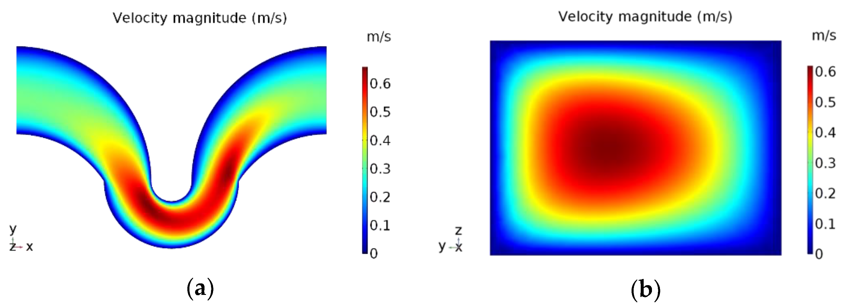
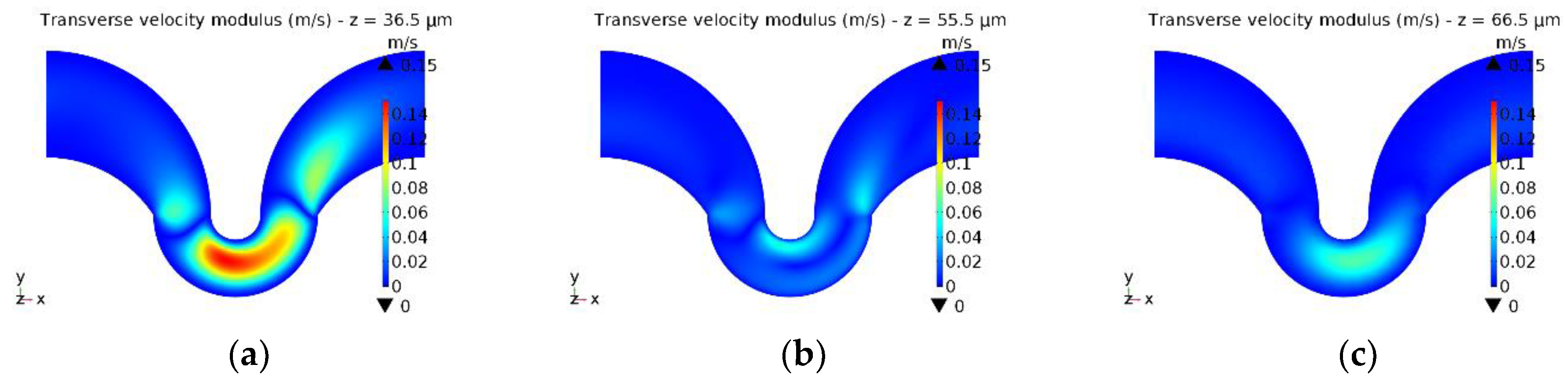
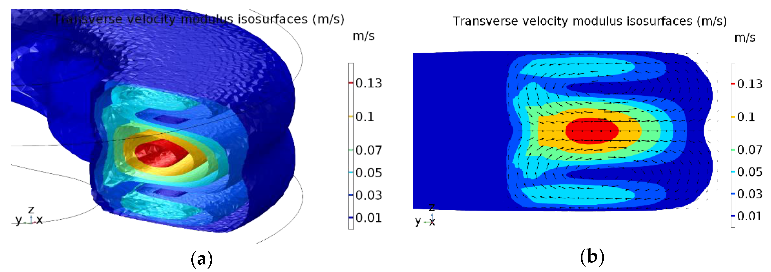
3.1. Stationary Solution for the Transverse Flow Field
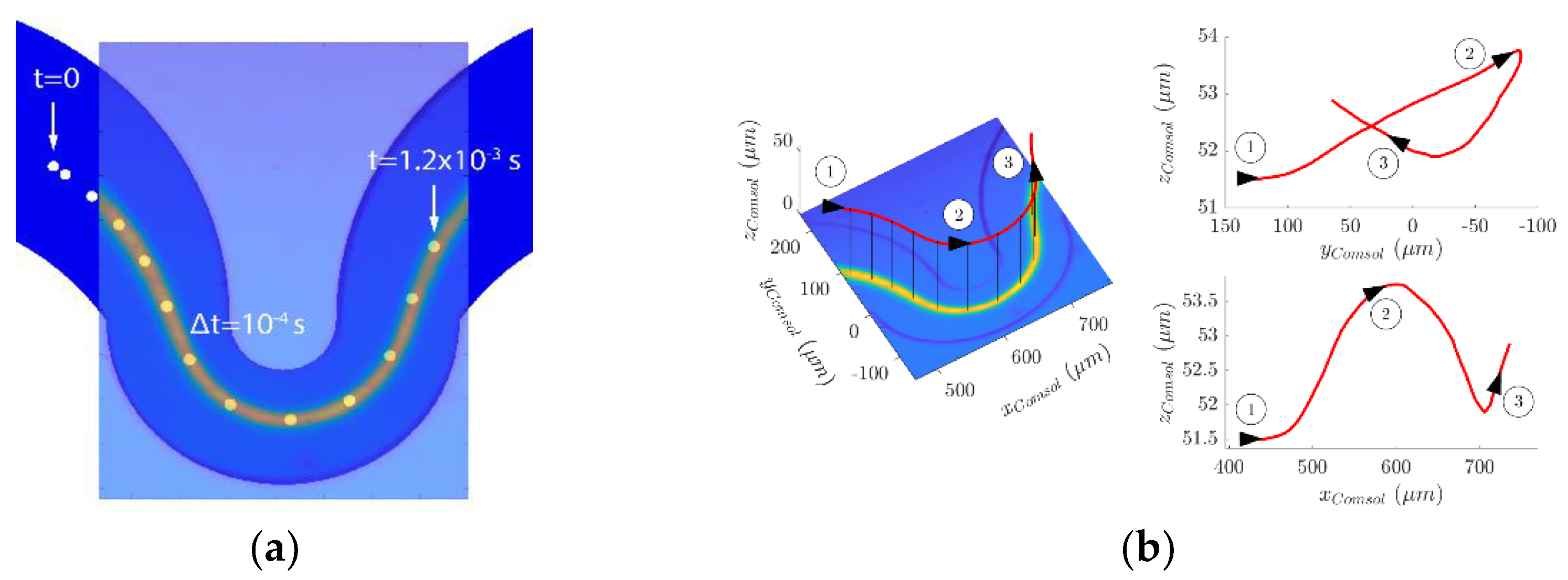
3.2. FSI Simulation
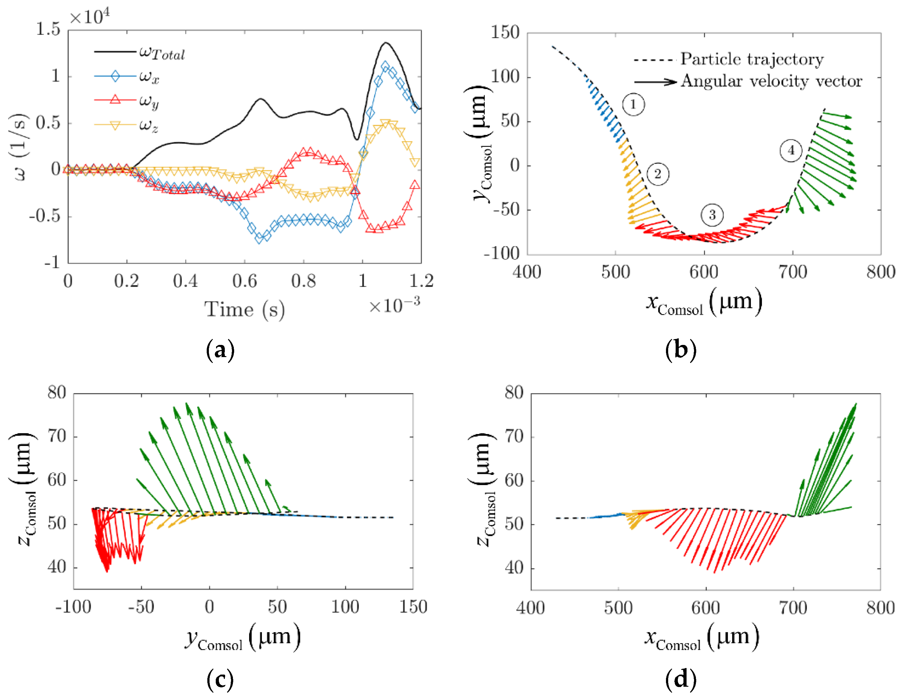
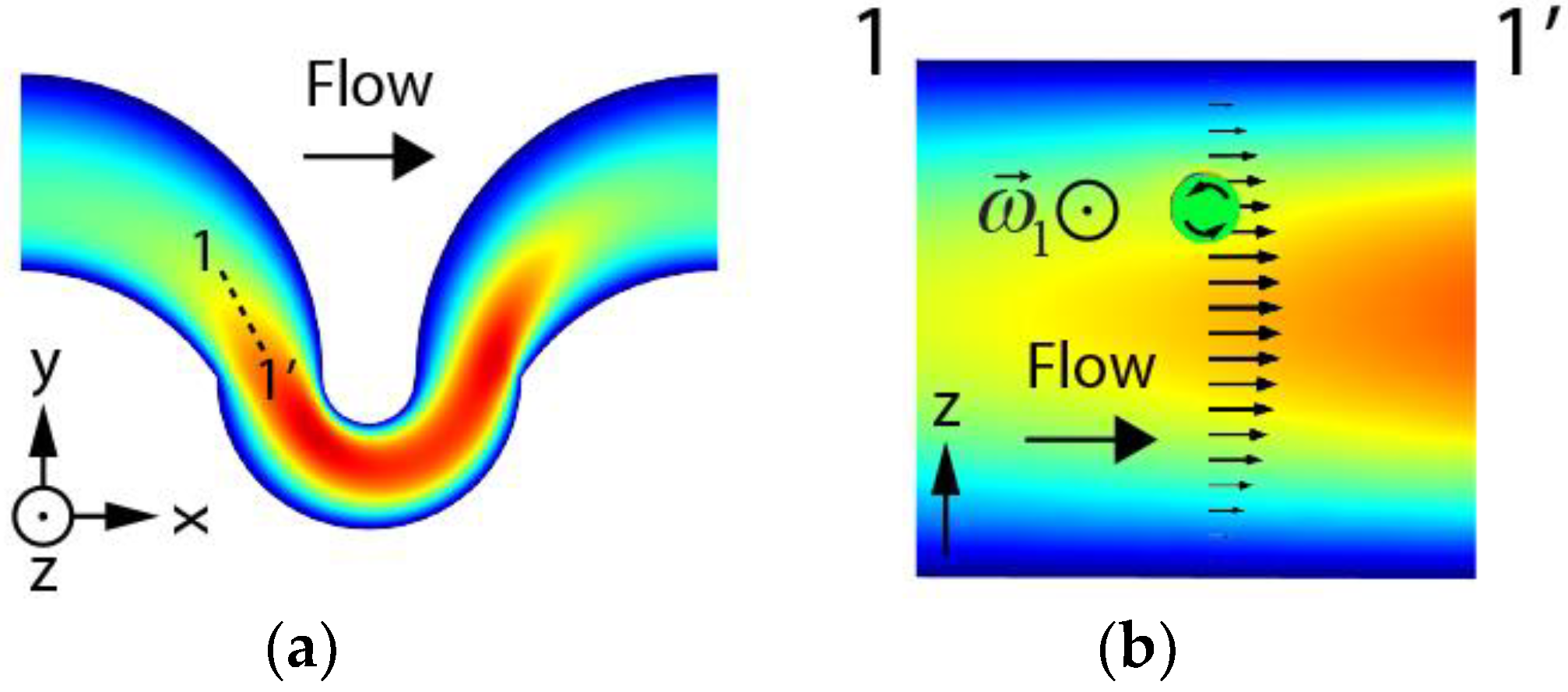
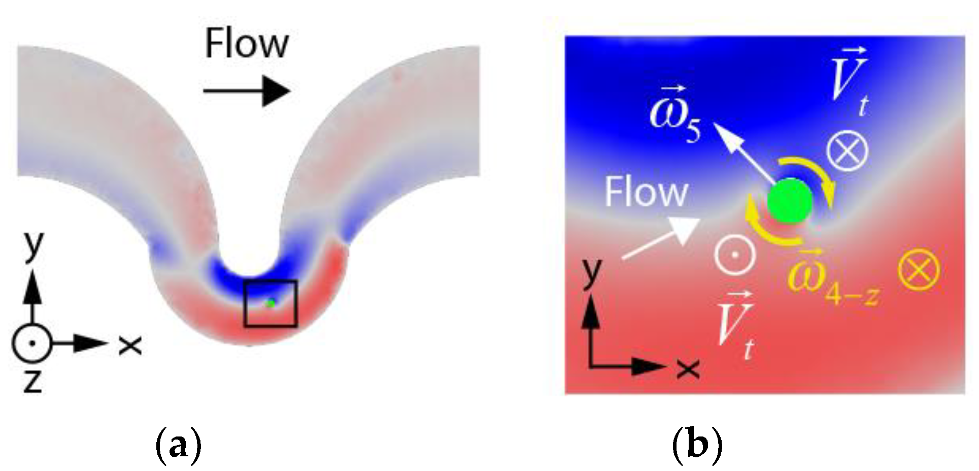
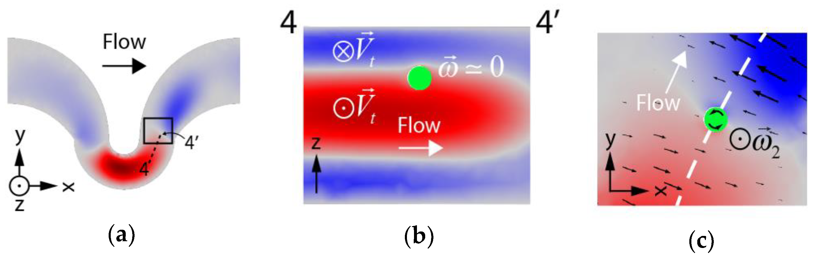
3.3. Particle Rotational Velocity Components
4. Conclusions
Author Contributions
Funding
Conflicts of Interest
References
- Poiseuille, J.L.M. Recherches sur les causes du mouvement du sang dans les vaisseaux capillaires. C. R. Acad. Sci. 1835, 6, 554–560. [Google Scholar]
- Tollert, H. Die Wirkung der Magnus-Kraft in laminaren Strömungen. Chem. Ing. Tech. 1954, 26, 141–150. [Google Scholar] [CrossRef]
- Taylor, M. The flow of blood in narrow tubes. Aust. J. Exp. Biol. 1955, 33, 1–16. [Google Scholar] [CrossRef]
- Maude, A.D.; Whitmore, R.L. The wall effect and the viscometry of suspensions. Br. J. Appl. Phys. 1956, 7, 98–102. [Google Scholar] [CrossRef]
- Saffman, P. On the motion of small spheroidal particles in a viscous liquid. J. Fluid Mech. 1956, 1, 540–553. [Google Scholar] [CrossRef]
- Di Carlo, D.; Irimia, D.; Tompkins, R.G.; Toner, M. Continuous inertial focusing, ordering, and separation of particles in microchannels. Proc. Natl. Acad. Sci. USA 2007, 104, 18892–18897. [Google Scholar] [CrossRef] [PubMed]
- Di Carlo, D.; Edd, J.F.; Irimia, D.; Tompkins, R.G.; Toner, M. Equilibrium separation and filtration of particles using differential inertial focusing. Anal. Chem. 2008, 80, 2204–2211. [Google Scholar] [CrossRef] [PubMed]
- Di Carlo, D. Inertial microfluidics. Lab Chip 2009, 9, 3038–3046. [Google Scholar] [CrossRef] [PubMed]
- Gossett, D.R.; Di Carlo, D. Particle focusing mechanisms in curving confined flows. Anal. Chem. 2009, 81, 8459–8465. [Google Scholar] [CrossRef] [PubMed]
- Kuntaegowdanahalli, S.S.; Bhagat, A.A.S.; Kumar, G.; Papautsky, I. Inertial microfluidics for continuous particle separation in spiral microchannels. Lab Chip 2009, 9, 2973–2980. [Google Scholar] [CrossRef] [PubMed]
- Oakey, J.; Applegate, R.W.; Arellano, E.; Di Carlo, D.; Graves, S.W.; Toner, M. Particle focusing in staged inertial microfluidic devices for flow cytometry. Anal. Chem. 2010, 82, 3862–3867. [Google Scholar] [CrossRef] [PubMed]
- Martel, J.M.; Toner, M. Inertial focusing dynamics in spiral microchannels. Phys. Fluids 2012, 24, 032001. [Google Scholar] [CrossRef] [PubMed]
- Sun, J.; Li, M.; Liu, C.; Zhang, Y.; Liu, D.; Liu, W.; Hu, G.; Jiang, X. Double spiral microchannel for label-free tumor cell separation and enrichment. Lab Chip 2012, 12, 3952–3960. [Google Scholar] [CrossRef] [PubMed]
- Cox, R.G.; Brenner, H. The lateral migration of solid particles in Poiseuille flow—I theory. Chem. Eng. Sci. 1968, 23, 147–173. [Google Scholar] [CrossRef]
- Ho, B.P.; Leal, L.G. Inertial migration of rigid spheres in two-dimensional unidirectional flows. J. Fluid Mech. 1974, 65, 365–400. [Google Scholar] [CrossRef]
- Vasseur, P.; Cox, R.G. The lateral migration of a spherical particle in two-dimensional shear flows. J. Fluid Mech. 1976, 78, 385–413. [Google Scholar] [CrossRef]
- Asmolov, E.S. The inertial lift on a spherical particle in a plane Poiseuille flow at large channel Reynolds number. J. Fluid Mech. 1999, 381, 63–87. [Google Scholar] [CrossRef]
- Subramanian, G.; Koch, D.L. Inertial effects on the transfer of heat or mass from neutrally buoyant spheres in a steady linear velocity field. Phys. Fluids 2006, 18, 073302. [Google Scholar] [CrossRef]
- Yang, C.; Zhang, J.; Koch, D.L.; Yin, X. Mass/heat transfer from a neutrally buoyant sphere in simple shear flow at finite Reynolds and Peclet numbers. AIChE J. 2011, 15, 1419–1433. [Google Scholar] [CrossRef]
- Hood, K.; Lee, S.; Roper, M. Inertial migration of a rigid sphere in three-dimensional Poiseuille flow. J. Fluid Mech. 2015, 765, 452–479. [Google Scholar] [CrossRef]
- Di Carlo, D.; Edd, J.F.; Humphry, K.J.; Stone, H.A.; Toner, M. Particle segregation and dynamics in confined flows. Phys. Rev. Lett. 2009, 109, 094503. [Google Scholar] [CrossRef] [PubMed]
- Amini, H.; Sollier, E.; Weaver, W.M.; Di Carlo, D. Intrinsic particle-induced lateral transport in microchannels. Proc. Natl. Acad. Sci. USA 2012, 109, 11593–11598. [Google Scholar] [CrossRef] [PubMed]
- Lee, W.; Amini, H.; Stone, H.A.; Di Carlo, D. Microfluidic crystals: Self-assembly and control of particle streams. Proc. Natl. Acad. Sci. USA 2010, 107, 22413–22418. [Google Scholar] [CrossRef] [PubMed]
- Wang, Q.; Yuan, D.; Li, W. Analysis of hydrodynamic mechanism on particles focusing in micro-channel flows. Micromachines 2017, 8, 197. [Google Scholar] [CrossRef]
- Liu, C.; Hu, G.; Jiang, X.; Sun, J. Inertial focusing of spherical particles in rectangular microchannels over a wide range of Reynolds numbers. Lab Chip 2015, 15, 1168–1177. [Google Scholar] [CrossRef] [PubMed]
- Liu, C.; Xue, C.; Sun, J.; Hu, G. A generalized formula for inertial lift on a sphere in microchannels. Lab Chip 2016, 16, 884–892. [Google Scholar] [CrossRef] [PubMed]
- Ladd, A.J.C. Numerical simultaions of particulate suspensions via a discretized Boltzmann equation. Part 1. Theoretical foundation. J. Fluid Mech. 1994, 271, 285–309. [Google Scholar] [CrossRef]
- Ladd, A.J.C. Numerical simultaions of particulate suspensions via a discretized Boltzmann equation. Part 2. Numerical results. J. Fluid Mech. 1994, 271, 311–339. [Google Scholar] [CrossRef]
- Ladd, A.J.C.; Verberg, R. Lattice-Boltzmann simulations of particle-fluid suspensions. J. Stat. Phys. 2001, 104, 1191–1251. [Google Scholar] [CrossRef]
- Yi, H. The lift on a spherical particle in rectangular pipe flow. Chin. J. Phys. 2013, 52, 174–184. [Google Scholar] [CrossRef]
- Kandhai, D.; Vidal, D.J.-E.; Hoekstra, A.G.; Hoefsloot, H.; Iedema, P.; Sloot, P.M.A. Lattice-Boltzmann and finite element simulations of fluid flow in a SMRX static mixer reactor. Int. J. Numer. Methods Fluids 1999, 31, 1019–1033. [Google Scholar] [CrossRef]
- Feng, Z.-G.; Michaelides, E.E. The immersed boundary-lattice Boltzmann method for solving fluid-particles interaction problems. J. Comput. Phys. 2004, 195, 602–628. [Google Scholar] [CrossRef]
- Peskin, C.S. The immersed boundary method. Acta Numer. 2002, 11, 479–517. [Google Scholar] [CrossRef]
- Jiang, D.; Tang, W.; Xiang, N.; Ni, Z. Numerical simulation of particle focusing in symmetrical serpentine microchannel. RSC Adv. 2016, 6, 57647–57657. [Google Scholar] [CrossRef]
- Le Tallec, P.; Gerbeau, J.-F.; Hauret, P.; Vidrascu, M. Fluid structure interaction problems in large deformation. C. R. Mec. 2005, 333, 910–922. [Google Scholar] [CrossRef]
- Wall, W.A.; Gerstenberger, A.; Gamnitzer, P.; Förster, C.; Ramm, E. Large Deformation Fluid-Structure Interaction—Advances in ALE Methods and New Fixed Grid Approaches; Springer: Berlin/Heidelberg, Germany, 2006; pp. 195–232. ISBN 978-3-540-34596-1. [Google Scholar]
- Bak, S.; Yoo, J.; Song, C.Y. Fluid-structure interaction analysis of deformation of sail of 30-foot yacht. Int. J. Naval Archit. Ocean Eng. 2013, 5, 263–276. [Google Scholar] [CrossRef]
- Tian, F.-B.; Dai, H.; Luo, H.; Doyle, J.F.; Rousseau, B. Fluid-structure interaction involving large deformations: 3D simulations and applications to biological systems. J. Comput. Phys. 2014, 258, 451–469. [Google Scholar] [CrossRef] [PubMed]
- Dubini, G.; Pietrabissa, R.; Montevecchi, F.M. Fluid-structure interaction problems in bio-fluid mechanics: A numerical study of the motion of an isolated particle freely suspended in channel flow. Med. Eng. Phys. 1995, 17, 609–617. [Google Scholar] [CrossRef]
- Barreiro, A.; Crespo, A.J.C.; Domínguez, J.M.; Gómez-Gesteira, M. Smoothed particle hydrodynamics applied in fluid structure interactions. WIT Trans. Built Environ. 2013, 129, 75–84. [Google Scholar] [CrossRef]
- He, Y.; Bayly, A.E.; Hassanpour, A. Coupling CFD-DEM with dynamic meshing: A new approach for fluid-structure interaction in particle-fluid flows. Powder Technol. 2018, 325, 620–631. [Google Scholar] [CrossRef]
- Warkiani, M.E.; Guan, G.; Luan, K.B.; Lee, W.C.; Bhagat, A.A.; Chaudhuri, P.K.; Tan, D.S.; Lim, W.T.; Lee, S.C.; Chen, P.C.; et al. Slanted spiral microfluidics for the ultra-fast, label-free isolation of circulating tumor cells. Lab Chip 2014, 14, 128–137. [Google Scholar] [CrossRef] [PubMed]
- Kim, T.H.; Yoon, H.J.; Stella, P.; Nagrath, S. Cascaded spiral microfluidic device for deterministic and high purity continuous separation of circulating tumor cells. Biomicrofluidics 2014, 8, 064117. [Google Scholar] [CrossRef] [PubMed]
- Zhang, J.; Yan, S.; Li, W.; Alici, G.; Nguyen, N.-T. High throughput extraction of plasma using a secondary flow-aided inertial microfluidic device. RSC Adv. 2014, 4, 33149–33159. [Google Scholar] [CrossRef]
- Zhou, J.; Kasper, S.; Papautsky, I. Enhanced size-dependent trapping of particles using microvortices. Microfluid. Nanofluid. 2013, 15, 611–623. [Google Scholar] [CrossRef] [PubMed]
- Javaid, M.U.; Cheema, T.A.; Park, C.W. Analysis of passive mixing in a serpentine microchannel with sinusoidal side walls. Micromachines 2018, 9, 8. [Google Scholar] [CrossRef]
- Rosaguti, N.R.; Fletcher, D.F.; Haynes, B.S. Laminar flow in a periodic serpentine channel. In Proceedings of the 15th Australasian Fluid Mechanics Conference, Sydney, Australia, 13–17 December 2004. [Google Scholar]
- Ahn, Y.-C.; Jung, W.; Chen, Z. Optical sectioning for microfluidics: Secondary flow and mixing in a meandering microchannel. Lab Chip 2008, 8, 125–133. [Google Scholar] [CrossRef] [PubMed]
- Nivedita, N.; Ligrani, P.; Papautsky, I. Evolution of secondary Dean vortices in spiral microchannels for cell separations. In Proceedings of the 17th International Conference on Miniaturized Systems for Chemistry and Life Sciences, Freiburg, Germany, 27–31 October 2013. [Google Scholar]
- Martel, J.M.; Toner, M. Inertial focusing in microfluidics. Annu. Rev. Biomed. Eng. 2014, 16, 371–396. [Google Scholar] [CrossRef] [PubMed]


© 2018 by the authors. Licensee MDPI, Basel, Switzerland. This article is an open access article distributed under the terms and conditions of the Creative Commons Attribution (CC BY) license (http://creativecommons.org/licenses/by/4.0/).
Share and Cite
Pedrol, E.; Massons, J.; Díaz, F.; Aguiló, M. Two-Way Coupling Fluid-Structure Interaction (FSI) Approach to Inertial Focusing Dynamics under Dean Flow Patterns in Asymmetric Serpentines. Fluids 2018, 3, 62. https://doi.org/10.3390/fluids3030062
Pedrol E, Massons J, Díaz F, Aguiló M. Two-Way Coupling Fluid-Structure Interaction (FSI) Approach to Inertial Focusing Dynamics under Dean Flow Patterns in Asymmetric Serpentines. Fluids. 2018; 3(3):62. https://doi.org/10.3390/fluids3030062
Chicago/Turabian StylePedrol, Eric, Jaume Massons, Francesc Díaz, and Magdalena Aguiló. 2018. "Two-Way Coupling Fluid-Structure Interaction (FSI) Approach to Inertial Focusing Dynamics under Dean Flow Patterns in Asymmetric Serpentines" Fluids 3, no. 3: 62. https://doi.org/10.3390/fluids3030062
APA StylePedrol, E., Massons, J., Díaz, F., & Aguiló, M. (2018). Two-Way Coupling Fluid-Structure Interaction (FSI) Approach to Inertial Focusing Dynamics under Dean Flow Patterns in Asymmetric Serpentines. Fluids, 3(3), 62. https://doi.org/10.3390/fluids3030062