Direct Numerical Simulation of Particles in Spatially Varying Electric Fields ^†

Abstract

A numerical scheme is developed to simulate the motion of dielectric particles in the uniform and nonuniform electric fields of microfluidic devices. The motion of particles is simulated using a distributed Lagrange multiplier method (DLM) and the electric force acting on the particles is calculated by integrating the Maxwell stress tensor (MST) over the particle surfaces. One of the key features of the DLM method used is that the fluid-particle system is treated implicitly by using a combined weak formulation, where the forces and moments between the particles and fluid cancel, as they are internal to the combined system. The MST is obtained from the electric potential, which, in turn, is obtained by solving the electrostatic problem. In our numerical scheme, the domain is discretized using a finite element scheme and the Marchuk-Yanenko operator-splitting technique is used to decouple the difficulties associated with the incompressibility constraint, the nonlinear convection term, the rigid-body motion constraint and the electric force term. The numerical code is used to study the motion of particles in a dielectrophoretic cage which can be used to trap and hold particles at its center. If the particles moves away from the center of the cage, a resorting force acts on them towards the center. The MST results show that the ratio of the particle-particle interaction and dielectrophoretic forces decreases with increasing particle size. Therefore, larger particles move primarily under the action of the dielectrophoretic (DEP) force, especially in the high electric field gradient regions. Consequently, when the spacing between the electrodes is comparable to the particle size, instead of collecting on the same electrode by forming chains, they collect at different electrodes.

1. Introduction

In recent years, considerable attention has been given to understanding the behavior of particles suspended within liquids because of their importance in a wide range of applications, e.g., self-assembly of micron to nano-structured materials, separation and trapping of biological particles [1], stabilization of emulsions, and the formation of fluids with adjustable rheological properties, etc. [2,3,4,5,6,7,8,9,10,11]. Future progress in these and related areas will critically depend upon our ability to accurately control the arrangement of particles for a range of particle types and sizes, including those of uncharged particles.

When a dielectric particle is subjected to a spatially non-uniform electric field it experiences an electrostatic force, called the dielectrophoretic (DEP) force. The DEP force arises because the particle becomes polarized and the polarized particle (or dipole) placed in a spatially varying electric field experiences a net force. This phenomenon itself is referred to as dielectrophoresis [2]. The force can be in the direction of the gradient of electric field or in the opposite direction. For a positively polarized particle the force is in the direction of the electric field gradient and for a negatively polarized particle the force is in the opposite direction to the gradient. In addition, the particle interacts electrostatically with other particles which can be modeled as dipole-dipole interactions. The dipole-dipole interactions are present even in a uniform electric field.

Dielectrophoresis is an important technique because it can be used to manipulate uncharged particles. Also, since the DEP force depends on the dielectric properties of the particle, the force is different on different kinds of particles. Therefore, in principle, DEP force can be used to separate particles with different dielectric properties [3]. For example, cancer cells can be separated from normal cells as they have different dielectric properties [12,13,14,15].

Here we present a direct numerical simulation (DNS) method based on the finite element method which can be used to study the motion of dielectric particles suspended in a dielectric liquid. The electric field can be uniform or nonuniform, e.g., the field in a dielectrophoretic cage is nonuniform. Direct numerical simulations are important for understanding the dependence of the DEP force-induced motion on the fluid and particle properties, and also for designing efficient microfluidic devices.

The point dipole (PD) approximation [2,14] which has been used in many past studies assumes that the particle is small compared to the length scale over which the electric field varies, and that the distance between the particles is much larger than the particle diameter. In this approximation, the electric force acting on a particle consists of two components, one due to dielectrophoresis, and the other due to the particle-particle interactions. The accuracy of the PD approximation decreases when the electric field varies significantly over a length scale comparable to the particle size and also when the distance between the particles is small.

The accuracy of the PD approximation can be improved by including higher order multipole moment terms in the force [16]. However, as shown in Reference [17], even when the multipole terms are included, it lacks the completeness of the Maxwell Stress Tensor (MST) method. In the latter method, the force is computed from the electric field that accounts for the presence of all particles in the computational domain and so the computed force incorporates multibody interactions [17]. The MST method is computationally demanding because the electric field has to be computed at each time step as the field changes when the particles move [18,19,20]. In Reference [21], an energy based method, which accounts for the presence of particles, was used to compute the force on the particles in a uniform electrical field. In this method, both far and near field interactions are included in the particle-particle force.

During the past 10 years, several new DNS approaches have been developed to model dielectrophoresis [22,23,24,25,26,27,28,29]. A scheme to study ac dielectrophoresis is described in Reference [30]. In this scheme, the ac electric field is obtained by solving the quasi-electrostatic form of the Maxwell equation from which the DEP force acting on the particles is obtained and the motion of particles in the fluid is simulated using the immersed boundary method. The scheme was used to study the motion of levitated particles and to evaluate the accuracy of the point dipole method. It was noted that in a given domain the accuracy of the PD method decreases with increasing particle size and that the accuracy diminishes in a high electric field gradient region. A numerical approach to study chain formation by particles with dissimilar electrical conductivities, sizes and shapes is described in [24]. An arbitrary Lagrangian-Eulerian (ALE)-based method was used in Reference [25,26] to study ac and dc dielectrophoresis in two-dimensions. The focus of this work was on understanding the mechanisms involved in particle assembly. A scheme based on the boundary-element method (BEM) was developed in Reference [27] to solve the coupled electric field, fluid flow and particle motion problems in the Stokes flow limit. A PD-based method in which the induced dipole moments within the particles are computed by accounting for the nearby particles, was developed in Reference [28]. There are several other studies in which only the DEP force lines in the devices were considered and the particle trajectories were estimated without considering the fluid-particle interactions [30,31].

Recently, in Reference [28], a multiphase model-based approach has been developed to study the motion of a large number of particles. The dielectrophoretic force in this approach is calculated using the point dipole approach, and the drag acting on the particles is modelled by Stokes law. The fluid flow induced due the motion of particles is not considered in this model. These model-based simulations allow us to study systems with thousands of particles which, at present, is not possible when a DNS approach is employed. However, a model-based approach may not accurately capture the underlying physics, and so the DNS or experimental results are needed to validate it.

In our DNS method, the exact equations governing the motion of the fluid and the particles are solved and subjected to the appropriate boundary conditions. The scheme uses a distributed Lagrange multiplier (DLM) method to enforce the rigid body motion constraint in the region occupied by the particles [32] and the electric force acting on the particles is computed using the point-dipole and Maxwell stress tensor approaches. One of the focuses of this paper is on the case where the particle size is comparable to the length scale over which the electric field varies. It is shown that the tendency of particles to form chains diminishes with increasing particle size, as the DEP force increases faster than the particle-particle interaction force. Thus, although particles come together to form chains when they are away from the electrodes, they may not collect at the same electrode as the neighboring electrode pulls some particles away from the first electrode. This happens because the presence of particles modifies the electric field, which changes the magnitude and direction of the DEP force.

2. Methods

The motion of particles suspended in fluids under the action of electric forces is governed by highly nonlinear coupled partial differential equations. We must solve the Navier-Stokes equation for the fluids which are coupled with the equation of motion for the particles and satisfy the boundary conditions. In addition, we must determine the electric field and calculate the electric force by integrating the Maxwell stress tensor over the surface of particles. The flow field and the electric field must be resolved at a scale smaller than the size of particles as well as in the gap between the particles. 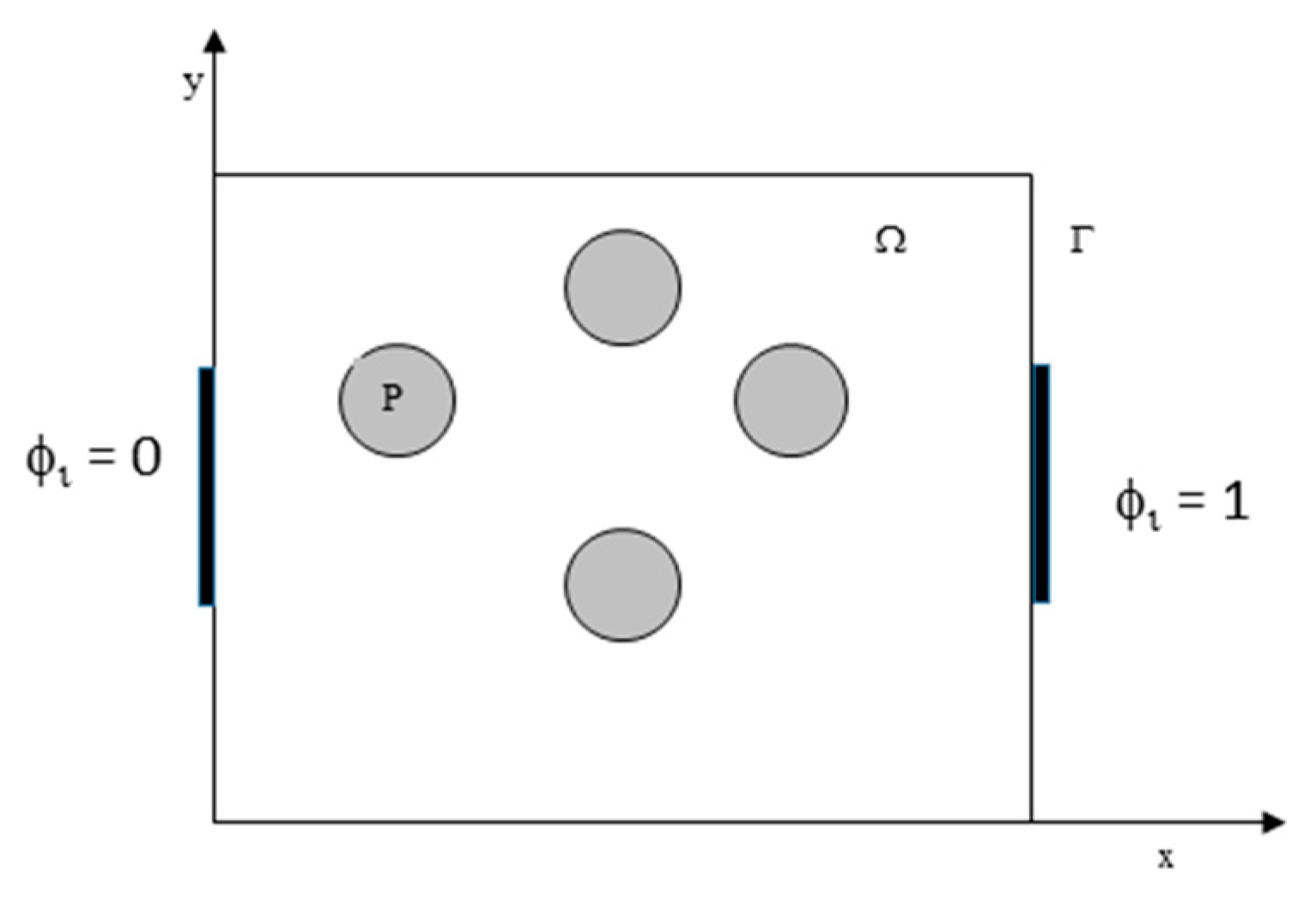Let us assume that there are N solid particles in the domain denoted by $\Omega$ and denote the interior of the i th particle by P_i(t), and the domain boundary by Г (see Figure 1). The momentum and mass conservation equations are

$${\rho }_L\left(\frac{\partial \mathbf{u}}{\partial t}+\mathbf{u}\cdot \nabla \mathbf{u}\right)=-\nabla p+\nabla \cdot (2\eta \mathbf{D})\mathrm{in}\Omega \backslash \overline{P\left(t\right)}$$

(1)

$$\nabla \cdot \mathbf{u}=0 \mathrm{in} \Omega \backslash \overline{P(t)}$$

(2)

where u is the fluid velocity, p is the pressure, η is the dynamic viscosity of the fluid, ${\rho }_L$ is the fluid density, D is the symmetric part of the velocity gradient tensor. The boundary conditions on the domain and the particle boundaries are:

$$\{\begin{array}{c}\mathbf{u}={\mathbf{u}}_L on \Gamma \\ \mathbf{u}={\mathbf{U}}_i+{\mathbf{\omega }}_i\times {\mathbf{r}}_i on {\Gamma }_{Pi},\hspace{1em} i=1,\dots ,N\end{array}$$

(3)

where U_i and ω_i are the linear and angular velocities of the i th particle, respectively, and Г_Pi = $\partial P_i(t)$ is the boundary of the i th particle.

The above equations are solved using the initial condition $u{|}_{t=0}=u_0$, where $u_0$ is the known initial value of the velocity.

The linear velocity U_i and the angular velocity ${\mathbf{\omega }}_i$ of the i th particle are governed by

$$m_i\frac{d{\mathbf{U}}_i}{dt}={\mathbf{F}}_i+{\mathbf{F}}_{E,i}$$

(4)

$$I_i\frac{d{\omega }_i}{dt}=T_i+T_{E,i}$$

(5)

$$\{\begin{array}{c}{\mathbf{U}}_i{|}_{t=0}=U_{i,0}\\ {\omega }_i{|}_{t=0}={\omega }_{i,0}\end{array}$$

(6)

where m_i and I_i are the mass and moment of inertia of the i th particle, respectively. F_i and T_i are the hydrodynamic force and torque acting on the i th particle, respectively, F_E,i is the electrostatic force acting on the i th particle and T_E,i is the electrostatic torque acting on the i th particle. In this paper, our focus is on the case of spherical particles, and so we do not need to keep track of the particle orientation. The particle velocities are then used to update the particle positions

$$\frac{d{\mathbf{X}}_i}{dt}={\mathbf{U}}_i$$

(7)

$${\mathbf{X}}_i{|}_{t=0}={\mathbf{X}}_{i,0}$$

(8)

where X_i,0 is the position of the i th particle at time t = 0.

2.1. Formulation of Algorithms

2.1.1. Point-Dipole and Maxwell Stress Tensor Approaches

In the PD approximation, the electric force acting on a particle is obtained by computing the net particle-particle interaction force and adding it to the dielectrophoretic force. The time averaged dielectrophoretic force in an AC electric field is [2,14]

$${\mathbf{F}}_{DEP}=2\pi a^3{\epsilon }_0{\epsilon }_c\beta \nabla {\mathbf{E}}^2$$

(9)

where a is the particle radius, ε_c is the dielectric constant of the fluid, ε₀ = 8.8542 × 10⁻¹² F/m is the permittivity of free space and E is the RMS (root mean square) value of the electric field. Equation (9) is also valid for a DC electric field, in which case E is simply the electric field intensity. The coefficient $\beta \left(\omega \right)$ is the real part of the frequency-dependent Clausius-Mossotti factor, given by

$$\beta (\omega )=\mathrm{Re}\left(\frac{{\epsilon }_p^{\ast }-{\epsilon }_c^{\ast }}{{\epsilon }_p^{\ast }+2{\epsilon }_c^{\ast }}\right)$$

(10)

where ${\epsilon }_p^{\ast }$ and ${\epsilon }_c^{\ast }$ are the frequency dependent complex permittivities of the particle and fluid, respectively. Here ${\epsilon }^{\ast }=\epsilon -j\sigma /\omega$ is the complex permittivity, where $\epsilon$ and $\sigma$ are the permittivity and conductivity, and $j=\sqrt{-1}$. Notice that the value of Clausius-Mossotti factor is between −0.5 and 1.0.

In a non-uniform electric field, the particle-particle interaction force on the i th particle due to the j th particle is obtained by accounting for the spatial variation of the electric field [33,34,35,36]

$${\mathbf{F}}_D=\frac{12\pi {\epsilon }_0{\epsilon }_c{\beta }^2{a}^6}{r^4}\left({\mathbf{r}}_{ij}\left({\mathbf{E}}_i\cdot {\mathbf{E}}_j\right)+\left({\mathbf{r}}_{ij}\cdot {\mathbf{E}}_i\right){\mathbf{E}}_j+\left({\mathbf{r}}_{ij}\cdot {\mathbf{E}}_j\right){\mathbf{E}}_i-5{\mathbf{r}}_{ij}\left({\mathbf{E}}_i\cdot {\mathbf{r}}_{ij}\right)\left({\mathbf{E}}_j\cdot {\mathbf{r}}_{ij}\right)\right).$$

(11)

Here r_ij is the unit vector from the center of i th particle to j th particle and r = |r_ij|.

We first obtain the electric potential by accounting for the presence of particle:

$$\nabla \cdot (\epsilon \nabla \phi )=0.$$

(12)

The boundary conditions on the particle surface are given by

$$\begin{array}{c}{\phi }_1={\phi }_2\\ {\epsilon }_c\frac{\partial {\phi }_1}{\partial n}={\epsilon }_p\frac{\partial {\phi }_2}{\partial n}\end{array}$$

(13)

where ${\phi }_1$ and ${\phi }_2$ are the electric potential in the liquid and particles, respectively. The electric field is then calculated using the expression

$$E=-\nabla \varphi ,$$

(14)

Then the Maxwell stress tensor is computed

$${\sigma }_M=\epsilon EE-\frac{1}{2}\epsilon (E•E)I$$

(15)

The electrostatic force and torque on the i th particle are given by

$$F_{E,i}={\displaystyle \underset{{\Gamma }_{P_i}}{\int }{\sigma }_M\times n_{i}ds}$$

(16)

$$T_{E,i}={\displaystyle \underset{{\Gamma }_{P_i}}{\int }(x-x_i)\times {\sigma }_M\cdot }{n}_{i}ds$$

(17)

where n_i is the unit outer normal on the surface of the i th particles and x_i is the center of the i th particle.

2.1.2. Dimensionless Equations and Parameters

Equations (1), (2) and (4) are nondimensionalized by assuming that the characteristic length, velocity, time, stress, angular velocity and electric field scales are a, U*, a/U*, ηU*/a, U*/a and E₀, respectively. The gradient of the electric field is assumed to scale as E₀/L, where L is the distance between the electrodes, which is taken to be the same as the domain width. The nondimensional equations for the liquid, after using the same symbols for the dimensionless variables, are:

$$\mathrm{Re}\left(\frac{\partial \mathbf{u}}{\partial t}+\mathbf{u}\cdot \nabla \mathbf{u}\right)=-\nabla p+\nabla \cdot \mathbf{\sigma }$$

(18)

$$\nabla \cdot \mathbf{u}=0 \mathrm{in} \Omega \backslash \overline{P(t)}$$

(19)

where $\sigma$is the dimensionless extra stress. If the PD approximation is used for evaluating the electrostatic force, the dimensionless equations for the particles become

$$\frac{dU}{dt}=\frac{6\pi \eta a^2}{m{U}^{\ast }}{\displaystyle \int \left(\frac{-pI+\sigma }{6\pi }\right)}\cdot nds+\frac{4\pi a^4{\epsilon }_0{\epsilon }_c\beta {\left|E_0\right|}^2}{m{U}^{\ast 2}L}E\cdot \nabla E+\frac{3\pi {\epsilon }_0{\epsilon }_c{a}^3{\beta }^2{\left|E_0\right|}^2}{4m{U}^{\ast 2}{\left|{\mathrm{r}}_{ij}\right|}^4}{F}_D$$

(20)

$$I_i\frac{d{\omega }_i}{dt}={\displaystyle \int (x-x_i)\times \left[(-pI+\sigma )\cdot n\right]dA}+\text{}{T}_{E,i}$$

(21)

In terms of the Maxwell stress tensor, they are:

$$\frac{dU}{dt}=\frac{6\pi \eta a^2}{m{U}^{\ast }}{\displaystyle \int (-pI+\sigma )\cdot nds}+\frac{\epsilon E_0^2{a}^3}{m{U}^{\ast 2}}{\displaystyle \int {\sigma }_M\cdot nds}$$

(22)

$$\frac{d\omega }{dt}=\frac{5\eta a^2}{2m{U}^{\ast }}{\displaystyle \int (x-x_i)\times (-pI+\sigma )\cdot nds}+\frac{\epsilon E_0^2{a}^3}{m{U}^{\ast 2}}{\displaystyle \int (x-x_i)\times {\sigma }_M\cdot nds}.$$

(23)

If the PD approximation is used, the above equations contain the following dimensionless parameters:

$$\mathrm{Re}=\frac{{\rho }_L{U}^{\ast }a}{\eta },P_1=\frac{6\pi \eta a^2}{m{U}^{\ast }},P_2=\frac{3\pi {\epsilon }_0{\epsilon }_c{\beta }^2{a}^3|E_0{|}^2}{4m{U}^{\ast 2}},P_3=\frac{4\pi {\epsilon }_0{\epsilon }_c\beta a^4|E_0{|}^2}{m{U}^{\ast 2}L},h^{\prime }=\frac{L}{a}.$$

(24)

Here Re is the Reynolds number, which determines the relative importance of the fluid inertia and viscous forces, P₁ is the ratio of the viscous and inertia forces, P₂ is the ratio of the electrostatic particle-particle interaction and inertia forces, and P₃ is the ratio of the dielectrophoretic and inertia forces. Another important parameter, which does not appear directly in the above equations, is the solids fraction of the particles; the rheological properties of ER (electrorheological) suspensions depend strongly on the solids fraction.

If the Maxwell stress tensor approach is used, an alternative parameter $P_E=\frac{\epsilon E_0^2{a}^3}{m{U}^{\ast 2}}$ which is a measure of the electrostatic forces is obtained in place of P₂ and P₃. This parameter is less informative than parameters P₂ and P₃, as it does not separately quantify the particle-particle and dielectrophoretic contributions. In flows for which the applied pressure gradient or the imposed flow velocity is zero, a characteristic velocity $U^{\ast }=\frac{2{\epsilon }_0{\epsilon }_c\beta a^2|E_0{|}^2}{3\eta L}$ can be obtained by assuming that the dielectrophoretic force and the viscous drag terms balance each other. For our simulation results, $U^{\ast }$is the maximum particle velocity.

In order to investigate the relative importance of the electrostatic particle-particle and dielectrophoretic forces, another parameter is defined:

$$P_4=\frac{P_2}{P_3}=\frac{3\beta L}{16a}$$

(25)

Equation (25) implies that if β = O(1) and L >> a, and so P₄ > 1, the particle-particle interaction forces will dominate, which is the case in most applications of dielectrophoresis. On the other hand, if β << O(1) and $\frac{\mathrm{L}}{\mathrm{a}}~$ O(1), and thus P₄ < 1, then the dielectrophoretic force dominates. The latter is the case for the larger sized particles considered in our simulations.

2.2. Finite Element Method

The computational scheme uses a distributed Lagrange multiplier method (DLM) for simulating the motion of rigid particles suspended in a Newtonian fluid [26,27]. In our implementation of the scheme, the fluid-particle system is treated implicitly using a combined weak formulation in which the forces and moments between the particles and fluid cancel. The flow inside the particles is forced to be a rigid body motion by a distribution of Lagrange multipliers. The time integration is performed using the Marchuk-Yanenko operator-splitting technique which is first-order accurate [19,21,26]. The domain is discretized using a tetrahedral mesh where the velocity and pressures fields are discretized using P₂-P₁ interpolations and the electric potential is discretized using P₂ interpolation. The scheme allows us to decouple its four primary difficulties:

• The incompressibility condition, and the related unknown pressure, This gives rise to a Stokes-like problem for the velocity and pressure distributions, which is solved by using a conjugate gradient method [32,37].
• The nonlinear advection term. This gives rise to a nonlinear problem for the velocity which is solved by using a least square conjugate gradient algorithm [32,37].
• The constraint of rigid-body motion in P_h(t), and the related distributed Lagrange multiplier. This step is used to obtain the distributed Lagrange multiplier that enforces rigid body motion inside the particles. This problem is solved by using a conjugate gradient method described in Reference [32,37]. In our implementation of the method we have used an H¹ inner product (see (35)) for obtaining the distributions over the particles, as the discretized velocity is in H¹.
• The equation for the electric potential. It is solved independently as it is not directly coupled with the momentum and mass conservation equations. Then the electric force is obtained using the Maxwell stress tensor approach [18,20].

2.3. Simulation Domains and Parameters

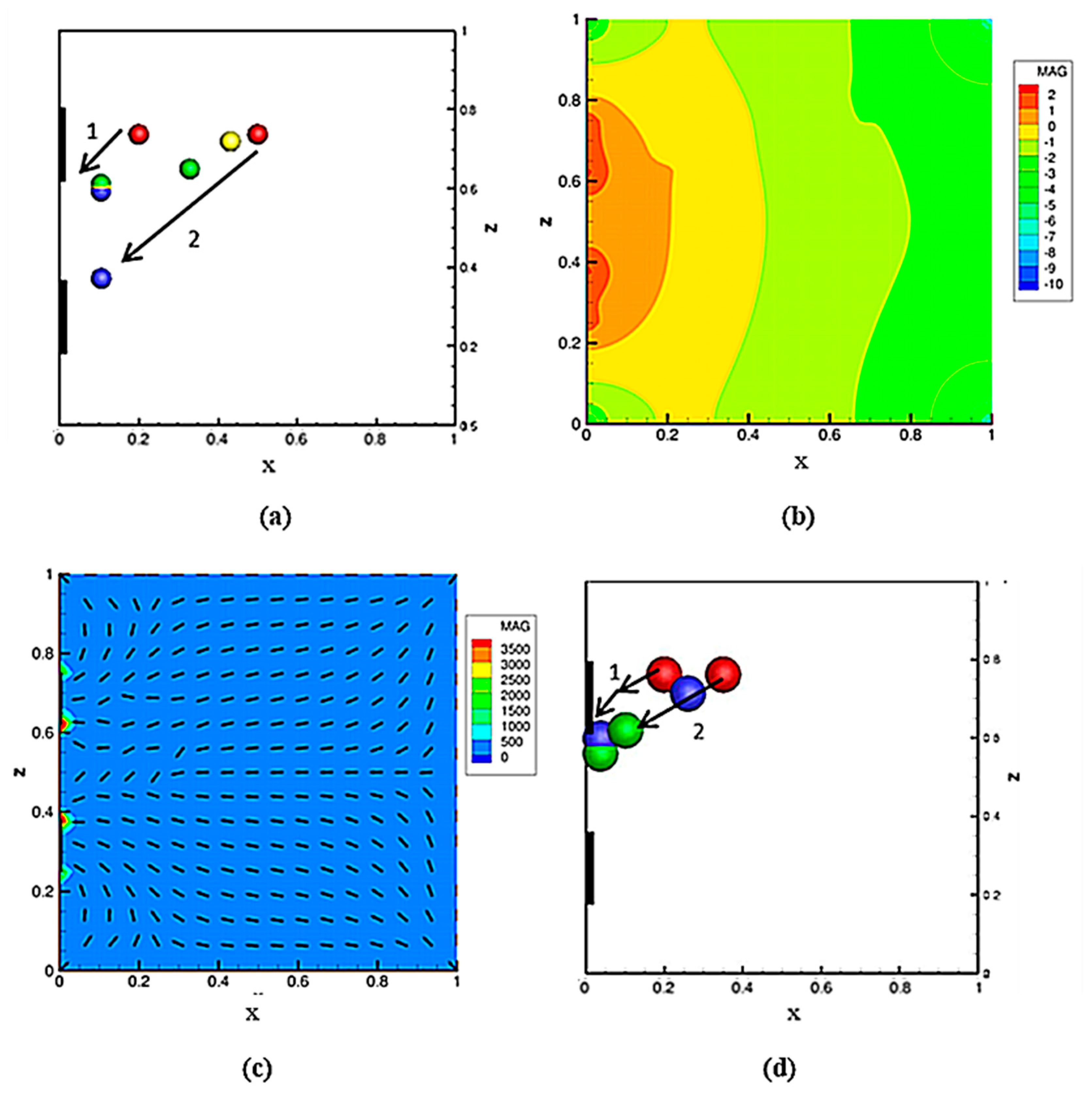
To test our finite element code, we conducted direct numerical simulations of the motions of two spherical particles in three-dimensional rectangular channels in which the electric field was non-uniform. In one of the domains, two electrodes were placed in one of the sides of the channel and in the second domain the electrodes were mounted on four walls of the channel.

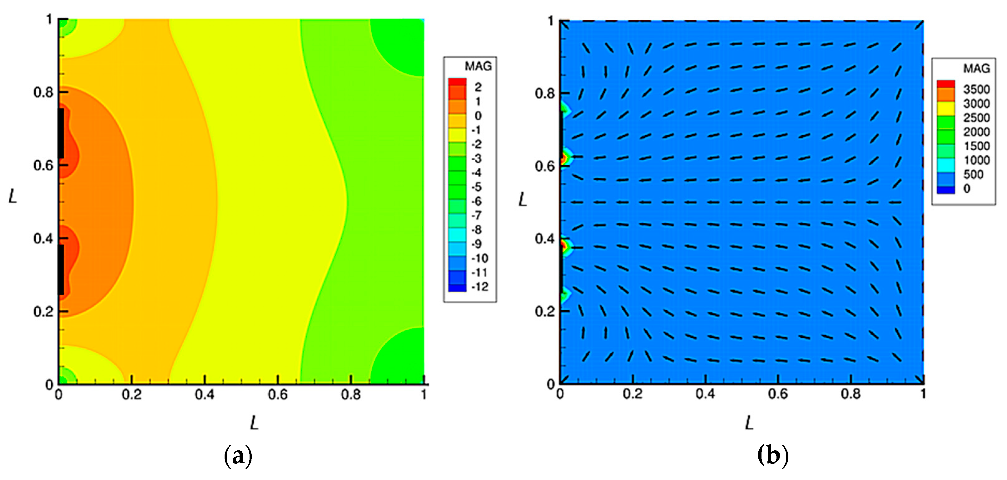
In the first domain, as shown in Figure 2 and Figure 3, two equally-spaced electrodes are embedded in the left wall parallel to the yz-plane. The electrodes are mounted in the middle of the wall such that they are equidistant from the domain centerline. Notice that the electrodes cover only a fraction of the wall area and so the electric field they generate in the domain is non-uniform. We also assume that the electrodes are mounted inside the walls so that they do not affect the fluid boundary conditions on the surface. The width of the electrodes in the y-direction is equal to the domain width which ensures that the electric field does not vary in the y-direction.

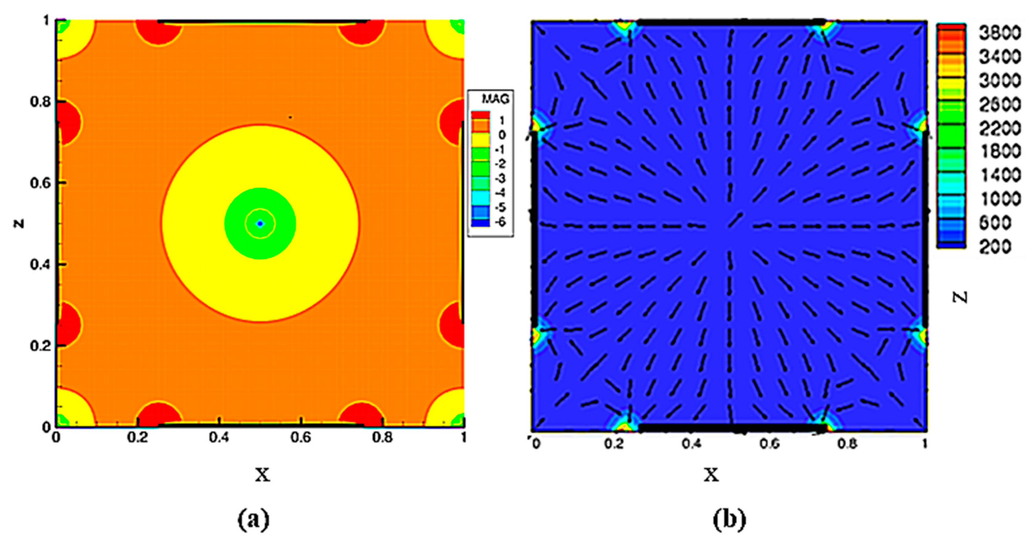
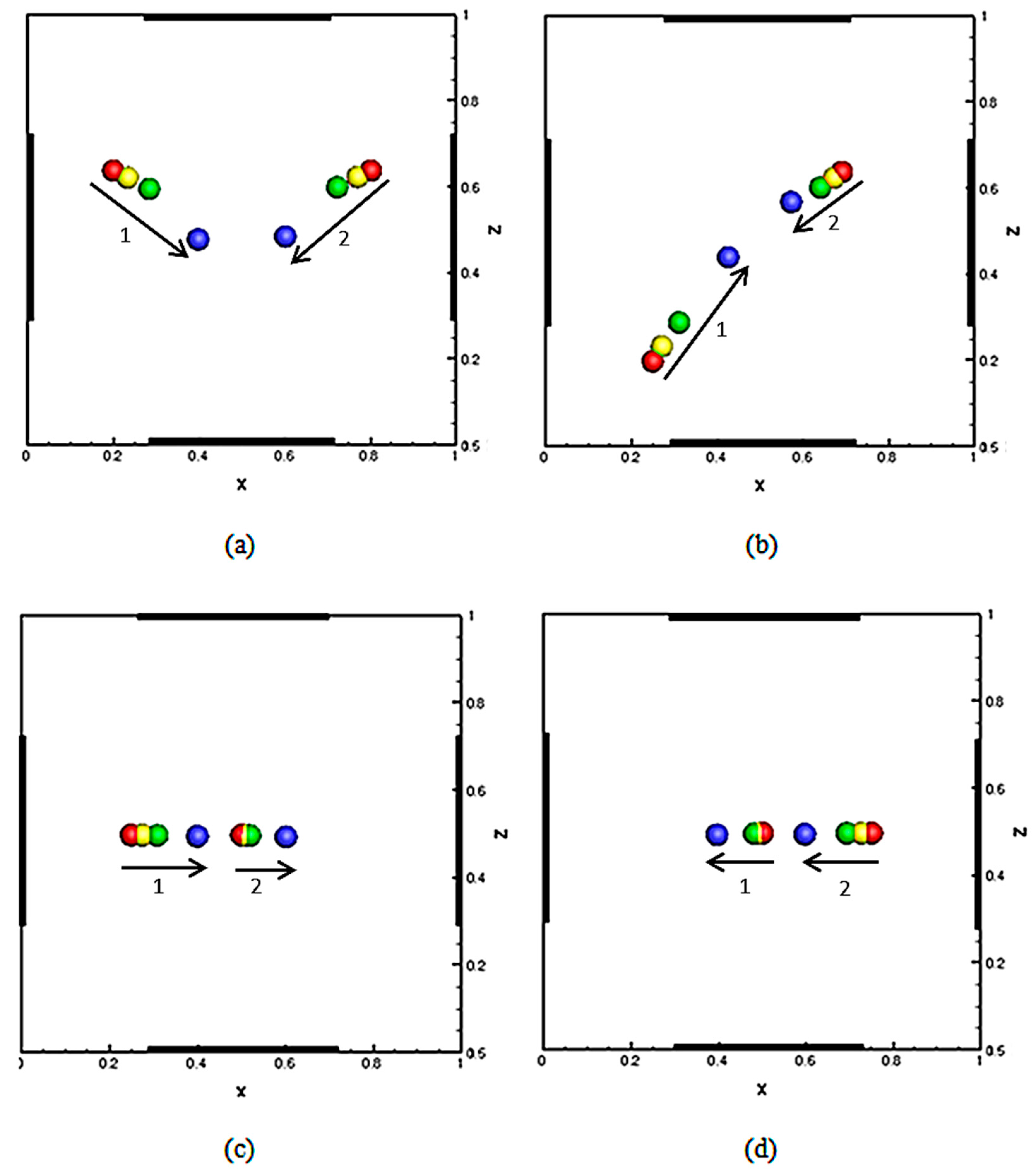
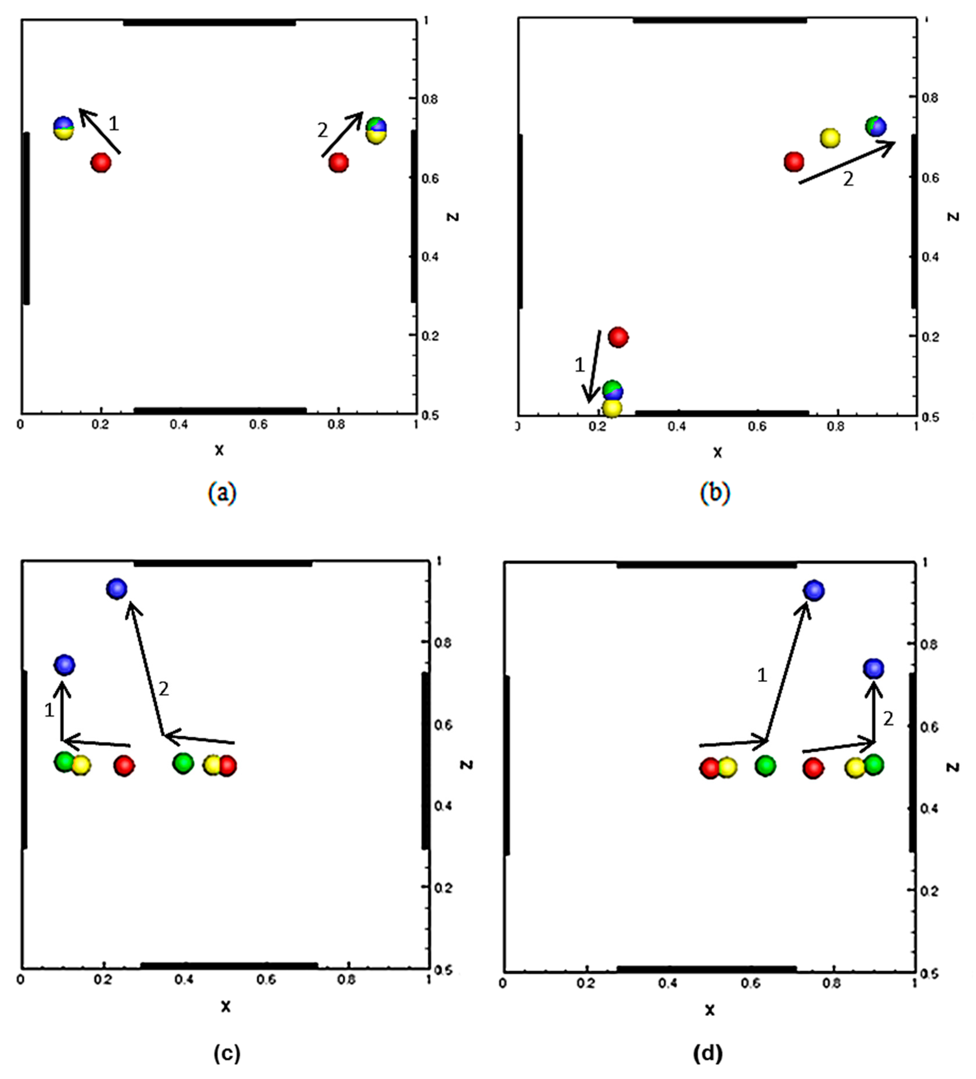
In the second domain, as shown in Figure 4, there are four electrodes mounted in the four side walls parallel to the yz- and xy-planes. The electrodes are mounted in the middle of the side walls and their depth is equal to the channel depth. The width of the electrodes is one and half the width of the domain sides. This domain can be used to capture a negatively polarized particle at its center and so it is referred to as the dielectrophorectic cage configuration.

In this paper, we will assume that the fluid density ${\rho }_L$ = 1.0 g/cm³ and that the particles are neutrally buoyant. The fluid viscosity is $\eta$ = 0.01 g/(cm·s), and both particles and fluid are non-conducting. The normalized dielectric constant of particles in our simulations is varied and that of the fluid is fixed at one. We will also assume that all of the dimensions reported in this paper are in mm and the time is in seconds. In our simulations, the initial fluid and particle velocities are assumed to be zero. At the domain walls the fluid velocity is assumed to be zero.

As shown in Figure 2, the dimensions of the computational domains in the x-, y- and z-directions are L, L/2 and L, respectively. All lengths are nondimensionalized by dividing by L. The particle radius and the distance between the particles are additional characteristic length scales in this problem. Note that the particle dielectric constant has been normalized with respect to the ambient liquid. Thus, a particle with ${\epsilon }_p$ > 1 is positively polarized and if ${\epsilon }_p$ < 1 the particle is negatively polarized. The radius of the circles used to represent particles is smaller than the actual particle radius.

3. Results and Discussion

3.1. Domain with the Electrodes Mounted in a Side Wall

The magnitude of the electric field distribution (|E|) on the xz-plane passing through the center of the domain is shown in Figure 2. The field is calculated for the case when the particles are not present and so the dielectric constant does not vary in the domain. Notice that the electric field distribution inside the channel is non-uniform and that the magnitude of |E| is maximum near the electrode edges and decreases with increasing distance from the electrodes. As discussed earlier in the paper, when particles are placed in a non-uniform electric field they are subjected to both the particle-particle interaction forces and the dielectrophoretic forces. Thus, their transient motions depend on the magnitudes and directions of $E \mathrm{and} E·\nabla E$, and also on the particles positions relative to the electric field direction.

Figure 2b shows that the gradient lines of the electric field magnitude (∇E²) point toward the electrodes, i.e., in the direction normal to the isovalues of$\left|E\right|$. Therefore, the DEP force on a particle with a dielectric constant greater than that of the suspending liquid is directed towards the electrodes; which is in the same direction as the lines of gradient of the electric field magnitude, as indicated by the arrows in Figure 2b. If the dielectric constant of the particle is smaller than that of the liquid, the DEP force is away from the electrodes.

3.2. Motion of Two Particles and Convergence Study

We next describe the transient motion of the two particles in the above non-uniform electric field and analyze the influence of the dipole-dipole and DEP forces. The dimensionless diameter of the particles in Figure 3a is 0.2. The initial positions of the particles are (0.2, 0.25, 0.88) and (0.5, 0.25, 0.88). The dimensionless parameters for the case presented are: Re = 0.652, P_E = 74.7, and P₄ = 0.117. Figure 3 shows the positions of the particles. The positions of the particles are shown at fixed time-intervals and the arrows show the direction of their motion. To track the movement of each particle, we use RYGB color-coding, with red showing the starting position and blue showing the final position. Initially, the particles moved closer because of the particle-particle interaction force, while moving toward the nearest electrode under the action of the dielectrophoretic forces. The particle on the left reached the electrode wall faster, as shown by the yellow circles, as the DEP force acting on it is greater than the particle-particle force because it is close to the upper electrode and the gradient of electric field is larger near the electrodes. The dielectrophoretic force increases as the distance between the particles and the electrode decreases, and the particle-particle force becomes relatively less in magnitude. The left particle is thus collected at the electrode much more quickly. The second set of particles initially moved slowly as the dielectrophoretic force acting on it was smaller, but its speed increased as it moved closer to the electrode. Notice that the electric field intensity and the magnitude and direction of ∇E² are modified by the particles (Figure 3c,d). The DEP force lines are no longer symmetric about the domain midplane, and the DEP force on the right particle is towards the lower electrode. The right particle, therefore, collected at the lower electrode. The particle-particle interaction force in this case is weaker than the DEP force which is expected since P₄ = 0.117. In Figure 3d, we present the results for the case where the particle diameter is 0.05, and P₄ = 0.468. Notice that in this case both particles collected at the upper electrode. This is due to the fact that the DEP force in this case is not stronger than the particle-particle force since the particle size is smaller.

Convergence Study

A convergence study is conducted to show that the numerical results obtained using the MST method converge when the time-step size is reduced and when the mesh is refined. To show convergence with the mesh refinement, we performed simulation on two mesh sizes. The first contained 139,425 nodes and the second 269,001 nodes. The times-step size used for these simulations is 1.0 × 10⁻⁴ s. To show convergence with the time-step size, simulations were performed for the time-step sizes of 2 × 10⁻⁴ s, and 1 × 10⁻⁴ s and 0.5 × 10⁻⁴ s. The number of nodes in these simulations is 139,425.

Figure 4 shows the x-position of the first particle as a function of time for two different mesh resolutions and three different time-step sizes. The figure shows that the trajectory of the particle remains virtually unchanged when the time step is reduced and also the mesh is refined. We may, therefore, conclude that the numerical results are converged and so are independent of the mesh refinement and the time step used.

3.3. Motion in a Dielectrophoretic Cage

As noted earlier, a dielectrophoretic cage is formed by placing electrodes in the four sides of a square-shaped domain as shown in Figure 5. The same voltage is applied to the opposite sides and the voltage applied to the adjacent sides is of the opposite sign. This device is of practical interest because it provides a way to trap one or more particles at the center of the device in a contactless fashion. The magnitude of the electric field (|E|) on the xz-plane passing through the middle of the domain is shown in Figure 5. Notice that there is a local minimum of |E| at the center of the domain, and that the field magnitude near the center increases with increasing distance from the center. The figure also shows that the electric field inside the cage is non-uniform, and that its gradient near the domain center is non-zero, except at the center itself where it is zero. Thus, the DEP force acting on a particle at the center is zero. The gradient of electric field magnitude points radially outward from the center and towards the electrodes (see Figure 5b). Therefore, if the dielectric constant of a particle is smaller than that of the liquid, the DEP force on the particle near the center will be towards the center, i.e., in the direction opposite to the gradient lines of the electric field magnitude. This implies that if the particle drifts away from the center, a restoring force acts on it which brings it back to the center. On the other hand, if the dielectric constant of the particle is greater than that of the liquid, the direction of the electric force is away from the center and so the particle moves away from the center and is carried to an electrode edge.

We next consider the motion of two particles in a dielectrophoretic cage, under the influence of positive and negative dielectrophoresis. For positive dielectrophoresis, ${\epsilon }_p>{\epsilon }_c=1$, and so the DEP force is in the direction of the force lines shown in Figure 5b, and for negative dielectrophoresis, ${\epsilon }_p<{\epsilon }_c=1$, the DEP force is in the direction of the force lines shown in Figure 4b.

3.3.1. Positive Dielectrophoresis $\left({\epsilon }_p=1.2\right)$

We first consider the case of positive dielectrophoresis, and so the dielectric constant of the particles (${\epsilon }_p=1.2)$ is assumed to be greater than that of the suspending fluid ${\epsilon }_c=1.0$. Figure 6 shows the positions of two particles for four different initial positions. The particles position at selected times are shown using a color-coded RYGB scheme, with red showing the starting position and blue showing the final position. The figure shows that the two particles are collected at a nearby electrode in all four cases.

Notice that in most cases particles are collected at the electrode edge that is nearest to them. However, a particle near the domain center can be pulled away from the nearest electrode by the particle-particle interaction force so that it is collected at an electrode edge that is farther away. For instance, in Figure 6c,d the final position of the particle at the center of the domain is determined by the initial position of the second particle which is near the center. The particle at the center is not subjected to a DEP force because the gradient of the electric field at the center is zero, and so if the second particle was not present it would remain at the center. In Figure 6c,d, the second particle pulls the particle at the center in its direction, and after it moves away from the center the DEP force also starts to act, and the DEP and particle-particles forces collectively determine its subsequent trajectory. The particle which was initially at the center is collected at the upper electrode because the particle-particle force in this case is smaller than the DEP force; P₄ = 0.117. The presence of particles modifies the DEP force lines, as was the case in Figure 3, and the DEP force drives the particle to the upper electrode. As discussed in Section 3.2, when the distance between the electrodes is comparable to the particle size, the tendency to form chains is weaker, especially near the electrodes, and so particles move individually.

These results are similar to the results in Reference [35] where the parameter P₄ was reduced by reducing β (which was varied independently by changing the frequency). Specifically, it was shown that since the particle-particle interaction force depends on the second power of β, and therefore becomes negligible compared to the DEP force, which itself depends linearly on β when β is small. This diminished the role of particle-particle interaction forces and, as a result, yeast particles moved individually, without forming chains, because of the DEP force. Here, on the other hand, the parameter P₄ has been reduced by increasing the particle size.

3.3.2. Negative Dielectrophoresis $\left({\epsilon }_p=0.2\right)$

In this subsection, we consider the case where the dielectric constant of the particles (${\epsilon }_p=0.2)$ is smaller than that of the suspending fluid ${\epsilon }_c=1.0$ and so particles undergo negative dielectrophoresis. For the four test cases shown in Figure 7, all other parameters including the domain size and the initial positions of the particles, are the same as for the case of the positive dielectrophoresis described in the previous subsection.

From Figure 7, we note that in all four cases the particles moved towards the domain center where the electric field magnitude is locally minimal (see Figure 5a). This also shows that the particle pair is stable at the domain center and that if the position is perturbed away from the center a restoring force acts which brings it back to the center. Thus, a dielectrophoretic cage can be used to position and hold negatively polarized particles at its center. Also, notice that the particles’ motion was in the opposite direction to the gradient line of the electric field magnitude (∇E²) as shown in Figure 4b. In fact, even after they are collected at the domain center, the particles maintained their orientations parallel to the gradient line along which they traveled. At the center, the gradient lines of (∇E²) emanate approximately radially outward, and so the particle pair is not subjected to a torque and its final orientation depends only on the initial orientation. Also, note that if a particle at the center is rotated, it is not subjected to a restoring torque and so it does not come back to its original orientation. The DEP force can only bring and hold circular particles at its center but cannot keep their orientations fixed.

3.4. Comparison with the Point-Dipole Approach

Finally, we compare the trajectory of a single particle in a DEP cage obtained using the MST method with that obtained using the point dipole (PD) method. We remind the reader that the PD method assumes that the presence of a particle does not alter the electric field and that the electric force on the particle can be obtained by using the value of ∇E² at its center. However, this is not the case for the results presented in Figure 5a and Figure 8 which show that the isovalues of log|E| are altered by the presence of a particle, and so the electric force given by the two methods is different. The difference between the forces given by the two methods is greater when the particle size is comparable to the length scale over which the electric field varies and the dielectric mismatch is larger.

In Figure 9, the particle trajectory and velocity computed using the two methods are shown as a function of time. The particle moves from its initial position (0.35, 0.25, 0.40) near the diagonal of the DEP cage to the bottom edge of the left electrode. Notice that although the final position given by the two force methods are approximately the same, the computed trajectories are different. For the point dipole method, the time taken to reach the equilibrium position was 0.15 s and for the MST method it was 0.13 s, implying that the point dipole method underestimates the electric force. This is consistent with the results reported in Reference [18], where the force acting on a fixed particle was computed using the MST and point dipole methods, i.e., the fluid and particle were not moving. It was noted that along the cage diagonal the PD method underestimates the force, and that the difference is larger when the particle size is larger. However, the PD method overestimates the force if the particle is displaced along the x- or y-direction from the center (also see [22]).

In Figure 10 and Figure 11, the particle positions and velocities obtained using the PD and MST methods are compared for the cases where the two particles are released away from their equilibrium positions in the cage. In Figure 10, the particles collected at an electrode edge where the magnitude of the electric field gradient is maximal. Notice that the final particle positions are slightly different for the two methods. This is due to the fact that the PD method does not account for the electric field modification caused by the presence of particles. Also, since the electric field gradient near the electrodes is larger, the differences in the trajectories for the two methods become larger as the particles move closer to the electrodes.

In Figure 11, the differences in the trajectories obtained using the PD and MST methods are relatively smaller. In this case, the particles undergo negative dielectrophoresis and move closer to the cage center where the magnitude of the electric field gradient is smaller (see Figure 8). These results show that in the regions where the gradient of the electric field intensity is larger or when the particle radius is comparable to the length scale over which the electric field varies, the difference between the trajectories obtained for the MST and the point-dipole methods is larger.

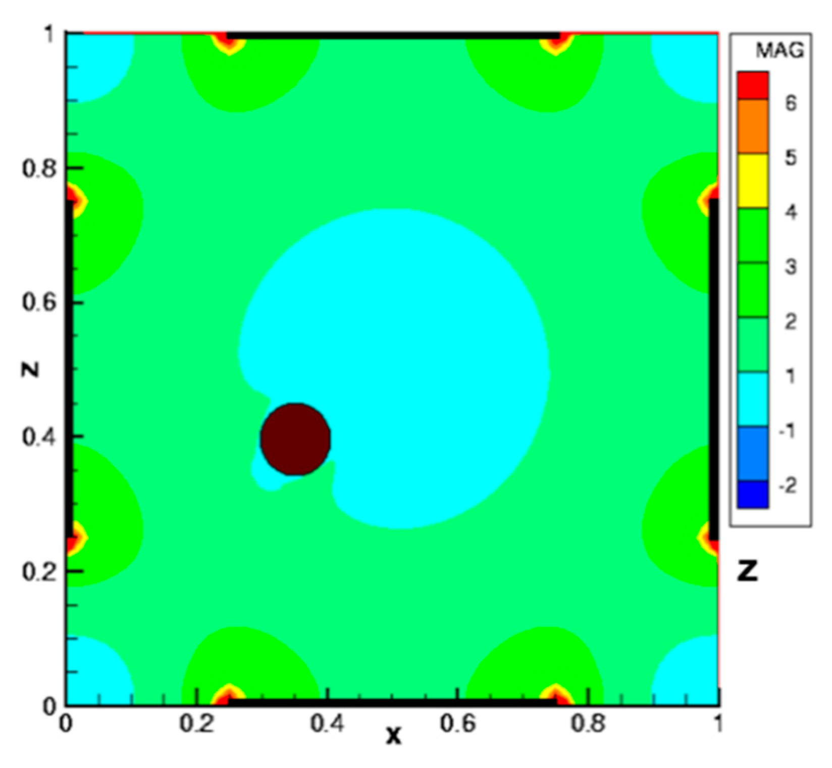
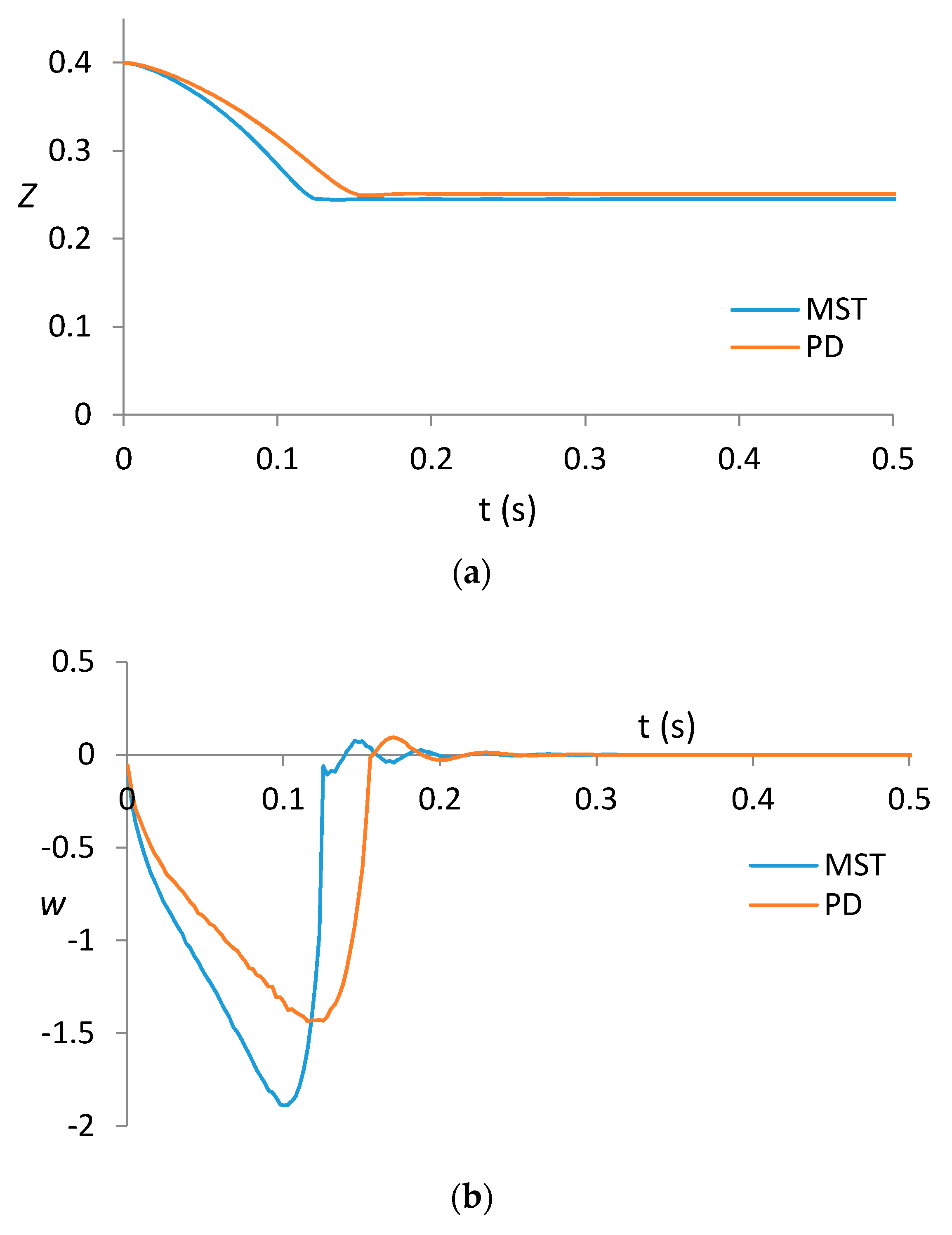
4. Conclusions

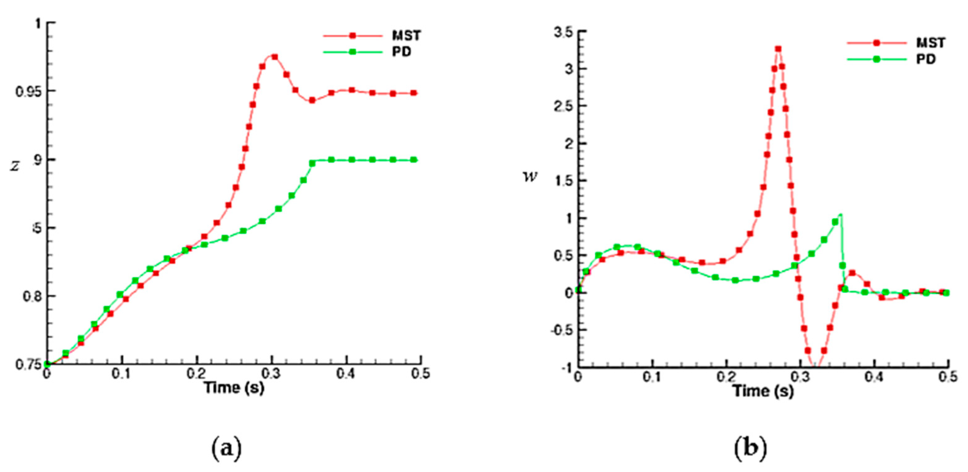
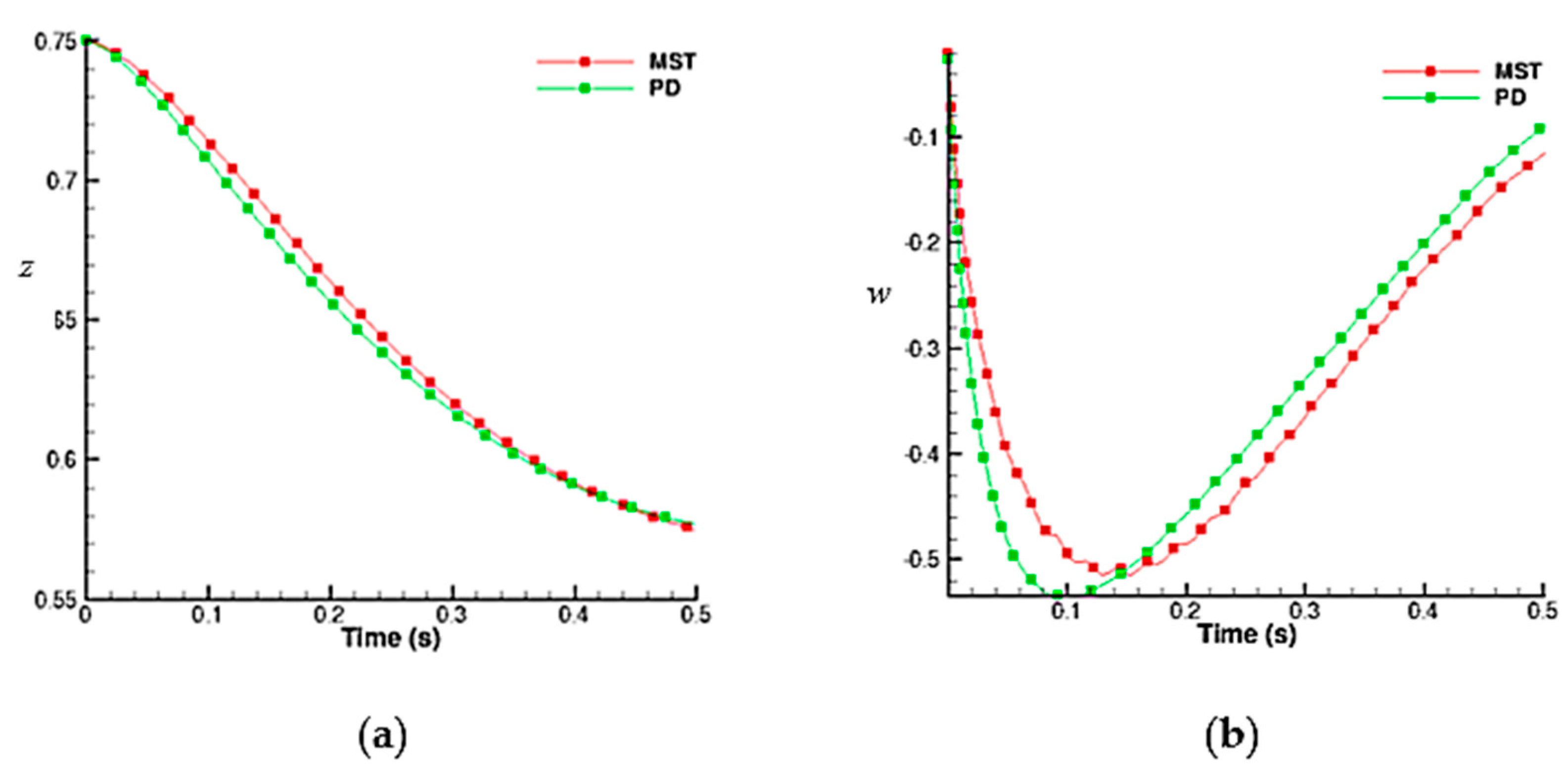
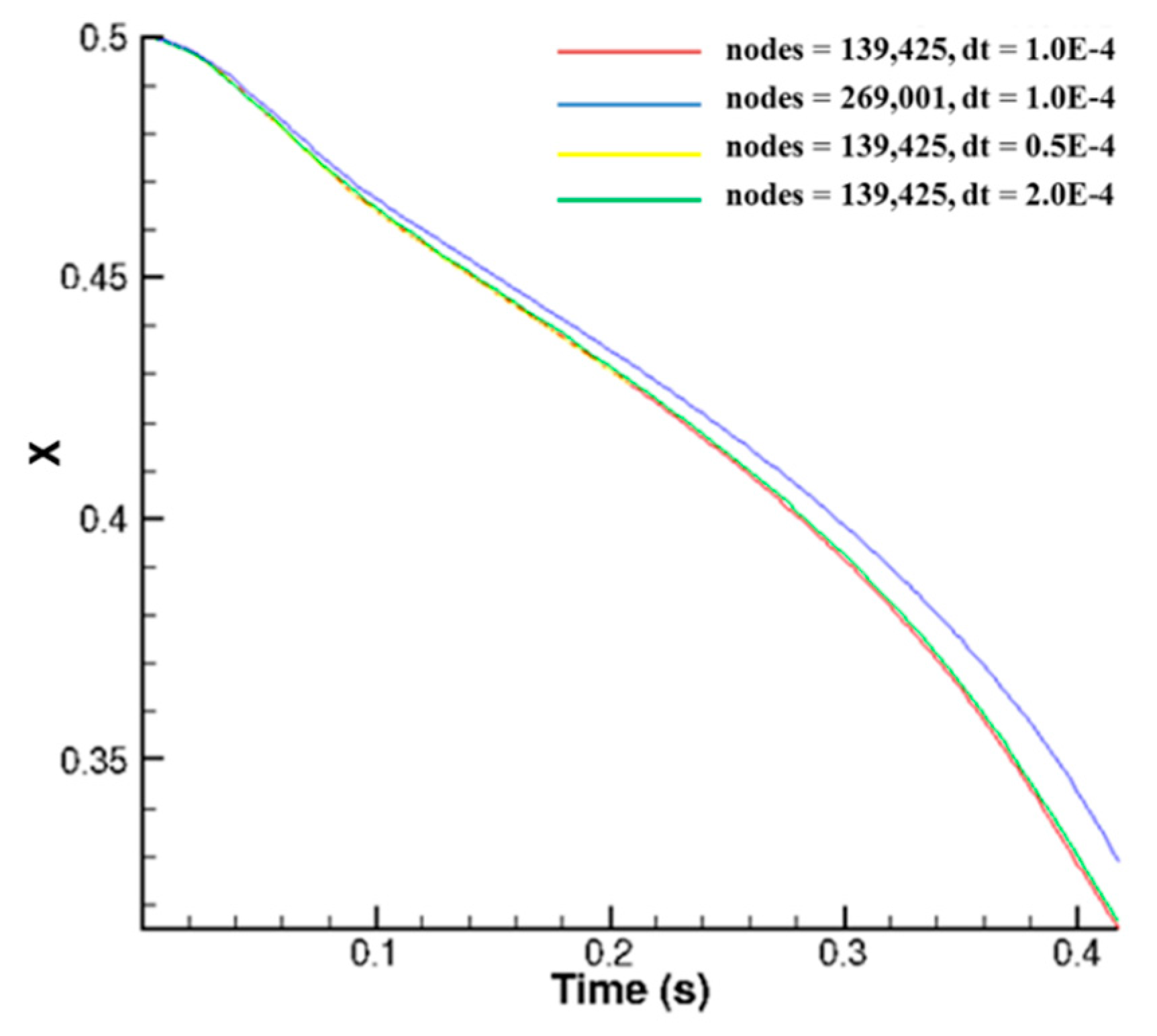
A finite element scheme based on the distributed Lagrange multiplier method is used to study the dynamical behavior of particles in a dielectrophoretic cage. The Maxwell stress tensor method is used for computing the electric forces acting on the particles, and the Marchuk-Yanenko operator-splitting technique is used to discretize in time. It is shown that a dielectrophoretic cage can be used to trap and hold negatively polarized particles at its center. If the particle moves away from the center of the cage, a resorting force acts on the particle towards the center. The cage also allows two particles to be trapped simultaneously at the center. The orientation of a trapped particle pair at the center depends on the initial positions of the particles, and in this sense, the pair orientation at the center is not fixed. Positively polarized particles, on the other hand, are trapped at the electrode edges depending on their initial locations. The particle trajectories obtained using the MST and point-dipole methods differ, but the final steady positions of the particles are approximately the same. The ratio of the particle-particle interaction and dielectrophoretic forces, P₄, decreases with increasing particle size which diminishes the tendency of particles to form chains, especially when they are close to the electrodes. Also, when the spacing between the electrodes is comparable to the particle size, instead of forming chains on the same electrode, particles collect at different electrodes. This is a consequence of the modification of the electric field due to the presence of particles, which is greater for larger particles.