Abstract
Windage (drag) losses have been found to be a key design factor for high power density and high-speed electric motor development. Inducing axial flow between rotor and stator is a common method in cooling the rotor. Hence, it is necessary to understand the effect on windage while forced axial airflow is in present in the air gap. The current paper presents results from experimental testing and modeling of a high-speed motor designed to operate at 30,000 revolutions per minute (RPM) and utilize axial air cooling of 200 Liters per minute (LPM) to cool the motor. Details of the experimental apparatus and computational fluid dynamics (CFD) modeling of the small gap narrow region of the stator/rotor are outlined in the paper. The experimental results are used to calibrate the CFD model. Results for windage losses, flow rate of cooling air, power and torque of the motor versus mass flow rate are given in the paper. Trade studies of CFD on the effect of inlet cooling flow rate, and parasitic heat transfer losses on the Taylor–Couette flow coherent flow structure breakdown are presented. Windage losses on the order of 20 W are found to be present in the configuration tested and simulated.
1. Introduction
The current work is motivated by a desire to understand the windage friction losses in small scale high power electric motors. This type of devices is of particular interest in applications involving electric and or hybrid vehicles. Understanding the windage losses in this type of devices can lead to more optimized configurations for use in industrial applications. Previous work into the windage losses of high-speed electric motors has been carried out. In the study of [], testing and numerical simulations for reducing the windage power loss of a high-speed rotor using a spiral grooved viscous vacuum pump combined with an aerodynamic step thrust bearing is proposed. The research of [] presents a strategy to mitigate the windage losses. Experimental tests using two machines combined with an existing stator and two rotors are carried out. As a result, a rotor with only the shrouds can greatly reduce the windage loss while keeping the maximum torque, power and motor efficiency at the high-speed region as it is. The work of [] presents the development of a very high-speed (200,000 RPM, 2000 W) slot-less permanent magnet motor (PM) using an analytical model. The model of [] includes magnetic fields, mechanical stresses in the rotor, electromagnetic power losses, windage power losses and the power losses in the bearings. The work of [] presents a study of windage losses for pulse generator rotors, which are quantified in terms of friction coefficients. From [], the plate friction coefficient is found to by proportional to a rotational Reynolds number by Re−0.2 while the cylinder friction coefficient is reported to be proportional to the Taylor number by Ta−1/2. Work in the area of fluid mechanics focusing on Taylor–Couette structures applicable to motor rotor design includes the work of [], wherein an experimental and numerical study is presented to a fluid confined between a rotating inner cylinder and a stationary outer one. The authors of [] investigate flow structures in cavities of two aspect ratios 3.76 and 1.04 with increasing Reynolds number. The work of [] presents numerical simulations for optimized stator and rotor shapes of interior permanent magnet type brushless motor for automotive cooling device in order to obtain better performance than the prototype. In contrast to the used air cooling, in the study of [], a PM motor uses circulated coolant of the rotor to enhance motor power per specific weight. The coolant circulates in the entire motor, from the housing to the rotor through the proposed coolant paths. Another coolant-based study is the work of [], which presents a thermal analysis for different rotor types according to the level of shield from eddy currents in order to achieve a safe thermal design of a high-speed permanent magnet (PM) motor designed for speed N = 31,500 RPM and power P = 130 kW. The research of [] presents 3D computational electromagnetic–thermal coupled analysis to analyze the effects of auxiliary cooling fans, called air-gap fans, on winding cooling in a large-capacity N = 27,000 RPM induction motor. Results from [] showed that flow rate distributed to the air gap was increased as the stagnant flow disappeared near the air gap because of the air-gap fans. From [], the heat transfer coefficients at the winding surface and air gap were increased up to 31% and 90%, and total winding cooling performance was improved, on average by 55%. The work of [] provides fundamental insight into the heat transfer behavior in the Poiseuille–Taylor–Couette flow field set-up between the rotor and the small gap of high-speed electric motors. Based upon the literature review above, it can be seen that the research and development of high-speed motor cooling is active and broad. The present work is unique in the regard of the very small narrow gap region being considered, i.e., the gap size is on the order of h = 2 mm and the gap to radius ratio is h/R = 0.045. To the author’s collective knowledge, the use of air cooling for the extremely small narrow gap region of the present configuration has not been addressed in the literature. In the literature, there is a wealth of information regarding resistive, hysteresis and bearing losses; however, there is no known formula or experimental data to predict the windage losses. The experimental and CFD modeling work presented here is designed to help engineers predict windage losses in high speed electric motor design. To this end, the body of the paper presents the experimental test apparatus and numerical simulations used for the present small gap high speed motor windage loss study.
2. Materials and Methods
2.1. Experimental Apparatus
The current work is focused on designing a high speed electric motor, which requires the designer to consider many power losses, such as resistive loss in copper winding, hysteresis losses in laminations, bearing losses and windage losses. The experimental apparatus of the present investigation is shown in Figure 1. Figure 1 shows the device under test, i.e., the motor, with inlet cooling air supply and exit air tubing, as well as the torque arm of the dynamometer used for testing.
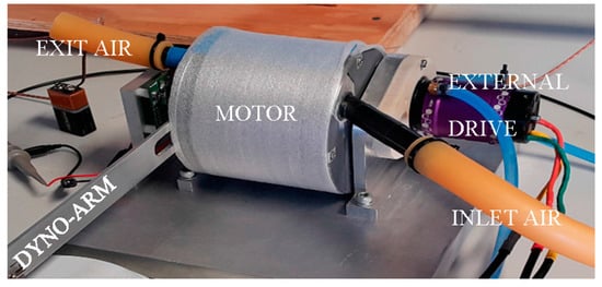
Figure 1.
Experimental apparatus.
The nomenclature of the experimental set-up is given in Figure 2. The outer round housing is made stationary and the inner rotor is supported by two ball bearings that mount onto the stationary housing. This present experiment takes out the electrical losses of the motor and study only the mechanical components.
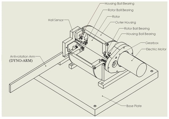
Figure 2.
Experimental apparatus nomenclature.
A detail of the motor test assembly is shown in Figure 3, while the actual test article for the rotor is shown in the picture of Figure 4.
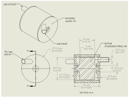
Figure 3.
Experimental apparatus rotor sub-assembly.
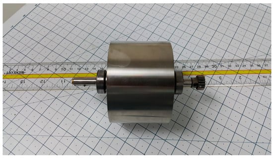
Figure 4.
Experimental apparatus rotor test hardware.
The balance experiment concentric cylinder setup is designed as follows: rotor with 87 mm O.D. and 60 mm length, stator/rotor air gap of 2 mm, the housing material is aluminum 6061 and the rotor material is stainless steel 304. This setup closely resembles a real size electric motor without copper windings. Two small ball bearings (ABEC5 deep-groove, bearing steel) with 10 mm I.D., 26 mm O.D. and 8 mm thickness. The apparatus of Figure 1, Figure 2, Figure 3 and Figure 4 closely mimics a real-size electric motor without copper windings. Many small electric motor stators are encapsulated with epoxy, in which the stator slots are all filled up and form a smooth round shape. This matches the experimental configuration at hand, which has a smooth round inner diameter. The electromagnetic field should not have effects on the air flow unless its field is strong enough to ionized the air particles. Most high-speed electric motors are under 1000 volts and the electromagnetic field effect can be ignored. Figure 5 shows the flowchart of the experimental procedure.
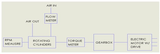
Figure 5.
Experimental procedure flow diagram.
2.2. Uncertainty Analysis
The uncertainty of the experimental apparatus is based upon the following dynamometer relationship:
where P = power, N = speed, F = force, l = moment arm and t = time. Using the method of [], the following total root-sum-square (RSS) uncertainty relationship is obtained from the power relationship of Equation (1) as follows:
The estimates of the elemental uncertainties are as follows. For the time measurement, 1 s is taken as the resolution of the scale of the time measurement device used: in this case, a stop-watch. The length scale for the dynamometer arm is taken as the smallest resolution of the ruler used: in this case 1/64 inch. The uncertainty of the force is taken as 2.5% from the load cell data used. The rotational speed is measured by a Hall effect sensor which outputs a square wave signal to the oscilloscope. The oscilloscope measures the square wave form’s peak to peak and display it as Hz on the screen, where 1 Hz = 1 RPM. The uncertainty of the speed is assumed to be 5% per the resolution of the oscilloscope trace used to post-process the speed transducer data. This is a worst-case assumption for the speed. Upon insertion of the numerical estimates for each uncertainty, . Future work would involve testing with a higher-accuracy tachometer.
2.3. Experimental Data Reducation Procedure
The test setup described above is specifically designed and fabricated to measure windage. In actual applications, there are bearing losses, windage losses and Joule heating losses. The literature [,] recognized this and presents a variety of methods to separate the various loss effects. Herein we have determined the average bearing losses and subtract them from the overall losses. The Joule heating and iron hysteresis losses are isolated by using an electric motor (external drive) to spin the test concentric cylinder system through a gearbox. For instrumentation, one thermocouple is placed at the inside of the air inlet tube before the air enters the housing, and another thermocouple is mounted at the inside of the air outlet tube after the air exits the housing. The air mass flow rate is measured by a vortex flow meter in the upstream of the air line before air enters the housing. Before actual performance and characteristic testing of the motor is performed, a small diameter rotor was made to replace the bigger diameter rotor for the purpose of rotor bearing friction measurement as shown in Figure 6 and Figure 7. Figure 6 shows the motor test apparatus using the small diameter bearing sized rotor. Figure 7 shows the hardware for the bearing-sized rotor test case. The use of the small rotor bearing apparatus allowed us to zero out the effect of bearing losses and focus specifically on windage losses. At 36,210 RPM, the bearing calculated bearing loss is 64 watts; at 36,600 RPM, the windage loss is 86.2 W.
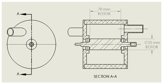
Figure 6.
Experimental apparatus bearing loss calibration fixture.
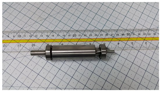
Figure 7.
Experimental apparatus bearing loss calibration rotor hardware.
The data reduction for the large rotor was accomplished by performing a torqued balance on the dynamometer.
The net torque on the rotor is zero when the rotor is either at rest or at constant steady speed. There are three source of torque that are acting on the rotor: (i) the input shaft torque, which is positive because it is delivering power to the system; (ii) the rotor ball bearings’ frictional torque that is against the rotor rotation and therefore has a negative sign; and (iii) the windage torque that is against the rotation of the rotor and also carries a negative sign. When under balance,
where the first term in Equation (4) is directly measured from the torque arm assembly, and the second rotor bearing term is determined from a calibration run for the bearing torque only (small diameter rotor test). The relationship between the large rotor (actual motor rotor mock-up) and the small rotor (bearing tar out mock-up) is given as follows:
where the “g” in Equation (5) denotes grams. Thus, from Equation (5), the scaling factor between using the test apparatus with the motor rotor mock-up versus the bearing mock-up is found to by k = 1.43. The small rotor is designed to mitigate the large rotor frictional torque. In other words, the windage torque cannot be measured unless bearing frictional torque can be measured. Therefore, the accuracy of the windage torque measurement is relative to how accurately we can measure the large rotor frictional torque. We cannot directly measure the large rotor frictional torque, because it would require us to spin the rotor in a vacuum to take out the windage effect. Hence, we used a small rotor. This leaves us the issue of the correction factor between the small rotor and the large rotor.
2.4. Spin Down Tests
Spin down tests were carried out in order to characterize the system performance. The scenario of no axial flow captures the maximum drag torque (due to bearing and windage), while the situation of induced axial flow sheds light on the time constant being altered due to induced flow, since there is expected to be more drag via the induced axial flow. Figure 8 shows the speed versus time spin down test with and without air cooling.
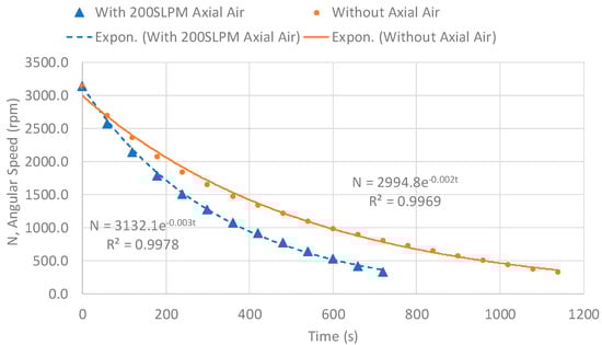
Figure 8.
Speed versus time rotor spin down test results.
From Figure 8, the time constant of the system is τ = 1/0.003 = 333 s, and τ = 1/0.002 = 500 s with and without 200 LPM of air cooling, respectively. Thus, we see that the effect of air cooling shortens the system time constant by 33%, as expected. Figure 9 shows the torque versus speed spin down curves with and without induced axial airflow. Figure 9 illustrates that with the introduction of annular axial air cooling, the slope of the motor torque speed curve increases when compared to the case without annular axial gap air cooling. Thus, using air cooling allows the motor to act a larger torque at a smaller rotational speed.
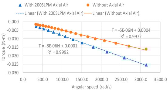
Figure 9.
Torque versus speed spin down rest results.
2.5. Numerical Modeling Methodology
The Navier–Stokes, conservation of energy, k-ω shear-stress transport (SST) turbulence model equations of motion are solved using the ANSYS Fluent (Version 14, ANSYS, Inc., Canonsburg, PA, USA) Computational Fluid Dynamics (CFD) software package []. The conservation equations solved by Fluent are as follows.
Conservation of mass:
where ρ is the fluid density and is the velocity vector.
Conservation of momentum:
where p is the static pressure, is the stress tensor, and , are the gravitational body force and miscellaneous body force terms, respectively.
Conservation of energy:
where = is the effective thermal conductivity, is the turbulent thermal conductivity, is the diffusion flux of species j. The first three terms on the right-hand side of Equation (8) denote the energy transfer due to conduction, species diffusion, and viscous dissipation, respectively. The source term includes the heat of chemical reaction and any other volumetric heat sources defined by the user. The total energy is given by
where the sensible enthalpy for an ideal gas is given by
Turbulence k-ω SST model:
where denotes the production of turbulent kinetic energy, denotes the generation of ω, and are the effective diffusivities of k and ω, respectively, and denote the dissipation of k and ω due to turbulence, respectively and denotes the cross-diffusion term, while and are user defined source terms. The effective diffusivity is modeled by
where the turbulent Prandtl numbers for k and ω are given as and below:
where the first blending function is given by
with
where y is the distance to the next surface and
The turbulent viscosity in the k-ω SST turbulence model is given by
where S is the strain rate magnitude, is defined as
where
and the model parameters = 6, . The second blending function is
The default model constants for the k-ω SST model outlined above are:
Per [], the wall boundary conditions for the k equation in the k-ω models are treated in the same manner as the k equation is treated when enhanced wall treatments are used with the k-ε suite of models. All boundary conditions for wall-function meshes correspond to the classical logarithmic wall function approach, while for the fine meshes, the appropriate low-Reynolds number boundary conditions is applied. For the value of ω, the value at the wall is specified by
where in the laminar sublayer
while in the logarithmic region
where the model constant . Per [], a wall treatment can be defined for the ω equation, which switches automatically from the viscous sublayer formulation to the wall function, depending on the grid. This improved blending is the default behavior for near-wall treatment. As pointed out in [] when using Fluent to model heat transfer in viscous flows within very narrow gaps, the viscous heating term of the energy equation must be enabled. The viscous self-heating is dictated by the Brinkman number:
2.6. Numerical Modeling Geometry, Grid, and Boundary Conditions
In this section of the paper, the CFD geometry, mesh and boundary condition prescription are discussed. Herein an ANSYS/Fluent CFD model was built to verify the windage of the heat generation windage loss experimental results presented above. The CFD model also used to predict/visualized development of Poiseuille–Taylor–Couette flow in stator/rotor narrow gap region. In the CFD analysis, we assume incompressible flow since the baseline inlet velocity of Re = 1626 (200 LPM) flow yields rotor outer edge axial speeds V = Rω lower than Ma = V/a = 0.3. Checking the Knudsen number, Kn = λ/h based upon the gap of h = 2 mm and for the air temperatures and pressures considered results in Kn << 0.0001, thus continuum flow is assumed. Figure 10 shows the CFD mesh used for the simulations. The mesh was comprised of 2.14M unstructured tetrahedral elements, with prismatic boundary layer refinement on all walls. Note the actual geometry of this motor is 87 mm O.D. and 60 mm length (roughly 3.5 inches by 2.5 inches), thus, in the author’s collective experience, a mesh on the order of 2M cells is adequate for these type of 3D simulations.
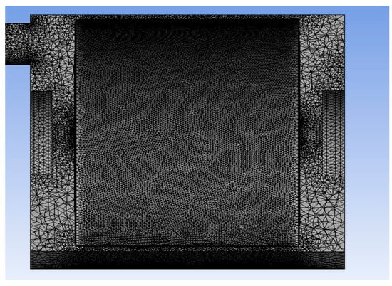
Figure 10.
Computational fluid dynamics (CFD) numerical mesh.
Prismatic grid layer inflation was used on the near wall boundary layer regimes of the flow field as shown in Figure 11 and Figure 12. Inflation layer settings for the rotor and stator were 4 layers of inflation, growth rate factor of 1.2 and 0.5 mm layer height. Details of the mesh in the corner area of the inlet to the gap region are shown in Figure 11. Figure 12 gives a zoomed in view of the prism layers on the rotor and stator side of the mesh.
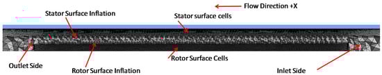
Figure 11.
CFD numerical grid prism inflation layers in narrow gap region.
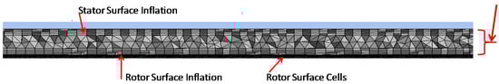
Figure 12.
CFD numerical grid prism inflation layers in narrow gap region.
Figure 13 shows the results of a mesh independence study.
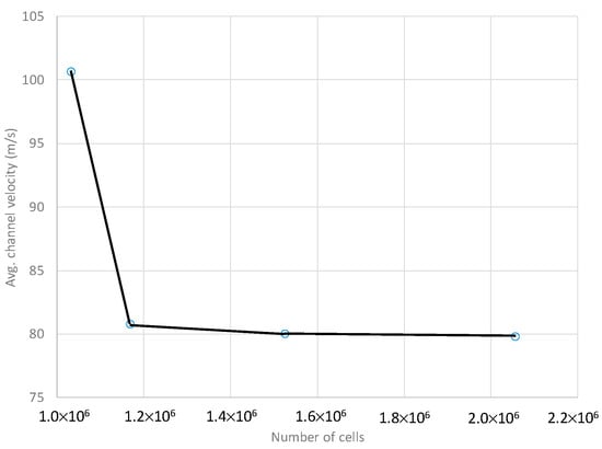
Figure 13.
Mesh independence study showing absolute mass averaged velocity in the channel versus number of computational cells used.
Figure 13 shows the fluctuation of the average velocity of the narrow gap versus the number of computational cells used. It should also be noted that a variety of other meshes were exercised during our investigation. The various mesh configurations examined are summarized in Figure 14.
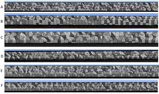
Figure 14.
Variety of meshes used: (A) 1,032,292 elements, no inflation, max. gap velocity = 166.717 m/s, (B) 1,026,658 elements, inflation (4 layers, 1.2 growth rate (GR), 1 mm layer height (LH)), max. gap velocity = 166.717 m/s, (C) 1,169,328 elements, inflation (4 layers, 1.2 GR, 0.5 mm LH), max. gap velocity = 166.717, (D) 1,526,354 elements, inflation (8 layers, 1.2 GR, 0.5 mm LH), (E) 2,057,948 elements, 4 cells across gap, inflation (4 layers, 1.2 GR, 0.5 mm LH), max. gap velocity = 166.721 m/s, (F) 2,139,700 elements, 4 cells across gap, inflation (4 layers, 1.2 GR, 0.5 mm LH), max. gap velocity = 166.721 m/s.
Here, we have adopted the use of an unstructured gird primarily due to the non-symmetric placement of the inlet relative to the outlet, thus lending no natural symmetry to the problem. The underlying issue of using a structured versus an unstructured grid comes down to a matter of choice. Figure 15 shows a schematic of the boundary conditions used. The inlet and outlet boundary conditions were pre-scribed as follows, inlet mass flow rate, exit zero pressure boundary condition. The walls of the rotor and motor case were assumed to be smooth walls. Figure 15 shows the boundary conditions prescribed to the CFD model.
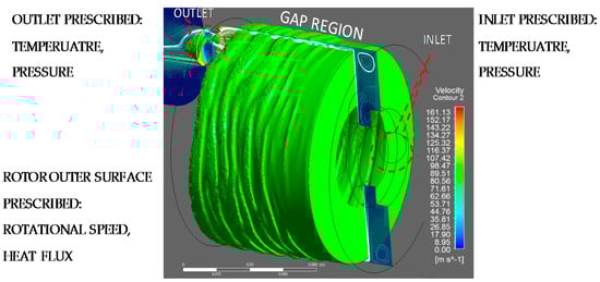
Figure 15.
CFD numerical simulation boundary condition prescription.
From Figure 15, the rotor’s rotational speed was applied using velocity BC. This is in contrast with using a rotating mesh, moving the reference frame, etc. The pros and cons of each method are discussed in []. For the results herein, we have adopted a wall velocity BC out of simplicity of implementation. The workstation used had the following specs: Intel i7 5960X 3.0 GHZ, 8-Core processor (Intel, Santa Clara, CA, USA) which was able to run 8–10 simultaneous calculations using 32 GB of random access memory (RAM). For graphics, an Nvidia Quadro workstation graphics card (Nvidia, Santa Clara, CA, USA) was used. The solution required 3000 iterations to resolve 90 s of physical of flow time, which took the solver just around 1.5 h of CPU time to solve 3D grids on the order of 2.2M cells. For the purposes of analyzing the simulation data and experimental data, a Reynolds number for Poiseuille–Taylor–Couette flow [] was used as follows:
where W = the axial annular gap flow rate, d = gap height, and ν = viscosity of the air. The Taylor number per [] is defined as follows
where R = inner rotor radius, ω = rotor speed. The flow pattern of the configuration under study is shown in Figure 13. The flow pattern under study is shown in Figure 16 for the baseline parameter of Ta = 3867, Re = 1664. This combination or Re, Ta numbers corresponds to the turbulent flow with vortices regime per her Schlichting []. It should be noted that the Re/Ta diagram of Schlichting [] is for d/R = 0.13 whereas the data herein is for a motor having rotor with 87 mm O.D. and 60 mm length, stator/rotor air gap of 2 mm or d/R = 0.046. Figure 16 is included to illustrate the non-symmetrical placement of the inlet and the outlet ports on the actual geometry, thus setting up a non-symmetrical flow filed. Figure 16 shows the isotherms (T = 305 K) and velocity streamlines from the CFD model.
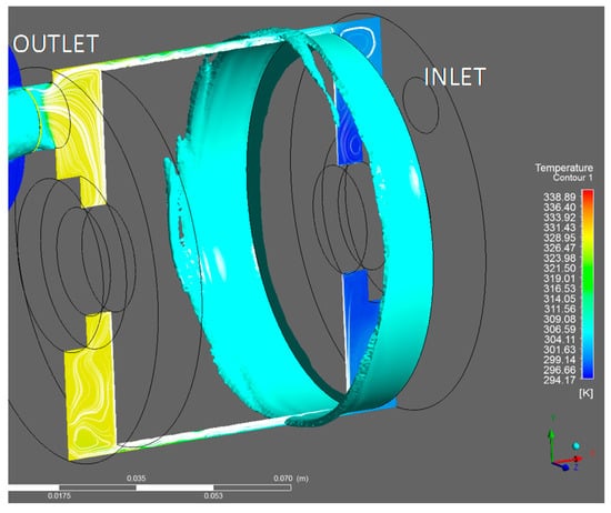
Figure 16.
CFD isotherms and streamlines.
The streamlines of Figure 16 are in qualitative agreement with those of the cylindrical configuration of []. Note also in Figure 16, then temperature increase from the inlet (295 K) to the outlet (329 K) is roughly 34 K, this increase in air temperature is affiliated with the windage losses of the rotor.
3. Results
This section of the paper presents the comparison of the experimental to the numerical simulation results for windage losses, the results of a numerical study of the effects of inlet mass flow rate on windage losses and the results of a numerical study on the effects of parasitic rotor heat transfer on the windage losses.
3.1. Windage Loss Results
Figure 17 shows the experimental and numerical prediction windage losses in the small gap region of the motor. The results of Figure 17 have been normalized using the average value of windage loss power found during the investigation; for instance, Pavg CFD = 59.31 W and Pavg Exp. = 57.4 W are the average windage losses found in the CFD simulation and experimental study, respectively. From Figure 14, the baseline operational scenario of Ta = 3867 (N = 36,000 RPM) rotor spin and Re = 1664 (200 LPM) inlet flow rate produces approximately 20 W of windage losses. This is in qualitative agreement with the studies of [,,] where 20 W to 30 W of windage losses are reported. From Figure 17, there is seen to be on average 14% agreement on average between the CFD and the experimental windage losses in the small narrow gap region of the motor. Thus, the CFD model is deemed to be correlated against the empirical data.
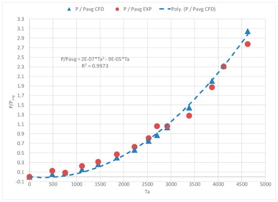
Figure 17.
Experimental and numerical windage for Re = 1664, Pavg CFD = 59.31 W and Pavg Exp. = 57.4 W.
Figure 18 presents the power windage loss findings in terms of a power coefficient traditionally defined in the turbo-machinery sector [] as follows:
where ρ is the air density, ω is the rotational speed of the motor, L denotes the height of the rotor cylinder, and R is the radius of the rotor. The motivation for the use of the power coefficient to scale windage losses herein is inspired by previous studies which have used variations of the power coefficient in their respective analyses [,]. The Taylor number, Ta in Figure 18, is as defined in Equation (31).
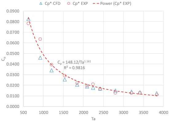
Figure 18.
Experiment and numerical windage results in terms of power coefficient.
The trends of Figure 18 are as follows: as the speed of the rotor ω is increased, the Taylor number increases, while the power is scaled by ω3 and thus the Cp factor decreases as the Taylor number Ta increases.
3.2. Inlet Mass Flow Rate Study
The CFD model was exercised in order to ascertain the effect of inlet mass flow rate on the windage losses set-up in the motor’s narrow gap region. The results of this study are shown in Figure 19.
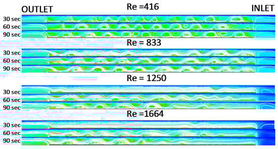
Figure 19.
CFD velocity streamlines versus inlet air supply mass flow rates for fixed rotation of Ta = 3867.
The flow structures reported in Figure 19 are the results of using unsteady computations. Details are from the first-order Euler time advancement numerical integration scheme of Fluent []. The snap-shots shown in Figure 19 are instantaneous contour plots at various time-steps: no sampling or averaging window was used when rendering Figure 19. From Figure 19, the main takeaway point is that the pseudo Poiseuille–Taylor–Couette cell structure evolution, velocity magnitude and streamline contours for Ta = 3867 (N = 36,000 RPM) cells become “bottle-necked” or “log jammed” at the cooling air outlet. This stack-up of vortices sheds light on the flaw of using forced air annular inlet cooling for high-speed motors, i.e., there will always be a point of diminishing return when using this type of heat transfer thermal control architecture. Figure 20 shows the effect of inlet air supply mass flow rate on the windage losses. The results of Figure 20 have been normalized with the average windage losses of 191.5 W.
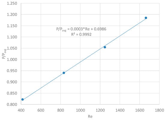
Figure 20.
Effect of inlet mass flow rate on windage losses for Pavg = 191.5 W.
The trend of Figure 20 indicates that the effect of inlet mass flow rate on the total windage losses of the rotor are a linear effect.
3.3. Rotor Parasitic Heat Loss Study
The CFD model was exercised in order to quantify the effect of parasitic heat flux on the windage losses set-up in the motor’s narrow gap region. The physical meaning of a parasitic heat flux is that of an unwanted loss in the system. This present analysis is an attempt to quantify and place an upper bound on the effects of parasitic heat losses in motors with small narrow gap rotor/stator regions. Figure 21 shows the isotherms for a parasitic heat flux of q” = 3541 W/m2 imposed onto the rotor, or in other words 100 W of parasitic heat flux applied to the outer surface of the motor rotor.
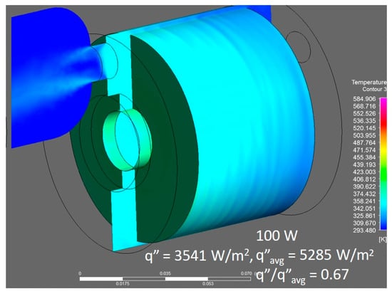
Figure 21.
Isotherms for rotor parasitic heat flux q” = 3541 W/m2.
Figure 22 shows the isotherms for a parasitic heat flux of q” = 7029 W/m2 imposed, or in other words 200 W parasitic applied to the outer surface of the motor rotor.
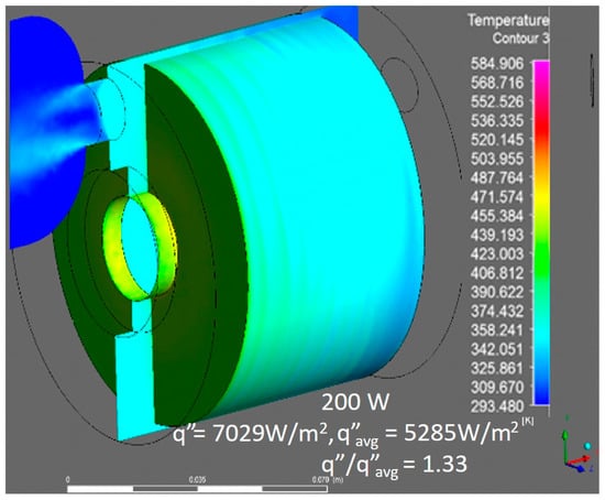
Figure 22.
Isotherms for rotor parasitic heat flux q” = 7029 W/m2.
Figure 23 shows the isotherms for a parasitic heat flux of q” = 10,570 W/m2 imposed onto the rotor, or in other words 300 W parasitic applied to the outer surface of the motor rotor.
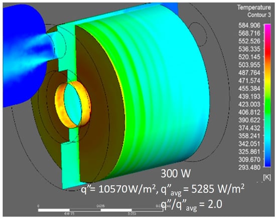
Figure 23.
Isotherms for rotor parasitic heat flux q” = 10,570 W/m2.
The results of Figure 24 have been normalized with the average parasitic losses 5295 W/m2. The trend of Figure 24 indicates that the effect of parasitic heat transfer losses on the total windage losses of the rotor are a quadratic effect. From the above results, as parasitic heat flux magnitude increases, the isotherms increase at the outer region and congregate at the outlet of the air supply. Thus, there is a substantial axial temperature gradient developed on the outer surface of the rotor when parasitic heat transfer occurs.
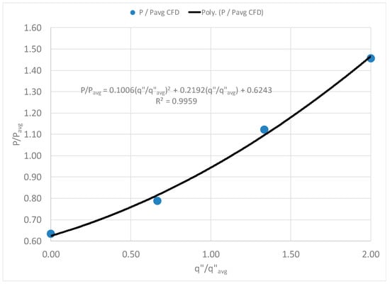
Figure 24.
Effect of parasitic heat flux on windage losses for Pavg = 152 W, q”avg = 5295 W/m2.
Figure 24 shows the impact of increased parasitic heat flux on the windage losses in the system.
4. Conclusions
This paper has presented the experimental and numerical findings of the windage losses in a high-speed electric motor. The paper has described the methodology used in the experimental and numerical simulation of the small gap electric motor. Thus, we see that the effect of air cooling is to shorten the system time constant by 33%. The electric motor’s rotor is designed to operate at 30,000 RPM with axial air flow on the order 200 LPM used to cool the motor. The experimental and numerical predictions for windage losses are found to be within 14% of agreement herein. The baseline value of 30,000 RPM rotor spin and 200 LPM inlet flow rate produces approximately 20 W of windage losses.
Author Contributions
Kevin Anderson directed the research study, Jun Lin engineered and built the test apparatus and performed the experimental measurements and Alexander Wong carried out the CFD numerical simulations.
Conflicts of Interest
The authors declare no conflict of interest.
References
- Asami, F.; Miyatake, M.; Yoshimoto, S.; Tanaka, E.; Yamauchi, T. A method of reducing windage power loss of a high-speed motor using a viscous vacuum pump. Precis. Eng. 2017, 48, 60–66. [Google Scholar] [CrossRef]
- Okada, Y.; Kosaka, T.; Matsui, N. Windage Loss Reduction for Hybrid Excitation Flux Switching Motors Based on Rotor Structure Design. In Proceedings of the Electric Machines and Drives Conference (IEMDC), Miami, FL, USA, 21–24 May 2017. [Google Scholar] [CrossRef]
- Pfister, P.D.; Perriard, Y. A 200,000 RPM, 2 kW Slot-less Permanent Magnet Motor. In Proceedings of the 2008 International Conference on Electrical Machines and Systems (ICEMS), Wuhan, China, 17–20 October 2008. [Google Scholar]
- Awad, M.N.; Martin, W.J. Windage Loss Reduction Study for TFTR Pulse Generator. In Proceedings of the 17th IEEE/NPSS Symposium on Fusion Engineering, San Diego, CA, USA, 6–10 October 1997. [Google Scholar] [CrossRef]
- Seelig, T.; Harlander, U.; Kielczewski, K.; Tuliszka-Sznitko, E.; Bontoux, P.; Egbers, C. Study of Transitional and Turbulent Flows in Rotor/Stator Cavities. In Proceedings of the 19th International Couette-Taylor Workshop, Cottbus, Germany, 24–26 June 2015. [Google Scholar]
- Yu, J.S.; Cho, H.W.; Choi, J.Y.; Jang, S.M.; Lee, S.H. Stator and rotor shape optimum design of brushless permanent magnet motor for automotive cooling device. In Proceedings of the 2012 IEEE Vehicle Power and Propulsion Conference (VPPC), Seoul, Korea, 9–12 October 2012; pp. 238–243. [Google Scholar] [CrossRef]
- Lee, K.H.; Cha, H.R.; Kim, Y.B. Development of an interior permanent magnet motor through rotor cooling for electric vehicles. Appl. Therm. Eng. 2016, 95, 348–356. [Google Scholar] [CrossRef]
- Kolondzovski, Z. Determination of critical thermal operations for high-speed permanent magnet electrical machines. Int. J. Comput. Math. Electr. Electron. Eng. 2008, 27, 720–727. [Google Scholar] [CrossRef]
- Kim, C.; Lee, K.S.; Yook, S.J. Effect of air-gap fans on cooling of windings in a large-capacity, high-speed induction motor. Appl. Therm. Eng. 2016, 100, 658–667. [Google Scholar] [CrossRef]
- Anderson, K.; Lin, J.; McNamara, C.; Magri, V. CFD study of forced air cooling and windage losses in a high speed electric motor. J. Electron. Cool. Therm. Control 2015, 5, 27–44. [Google Scholar] [CrossRef]
- Kline, S.A.; McClintock, F.A. Describing uncertainties in single-sample experiments. Mech. Eng. 1953, 75, 3–8. [Google Scholar]
- Concli, F. Pressure distribution in small hydrodynamic journal bearings considering cavitation: A numerical approach based on the open-source CFD code OpenFOAM®. Lubr. Sci. 2016, 28, 329–347. [Google Scholar] [CrossRef]
- Concli, F. Thermal and efficiency characterization of a low-backlash planetary gearbox: An integrated numerical-analytical prediction model and its experimental validation. Proc. Inst. Mech. Eng. Part J J. Eng. Tribol. 2016, 230, 996–1005. [Google Scholar] [CrossRef]
- ANSYS Fluent User Manuals; V14. 0 ANSYS. ANSYS Inc.: Cannosburg, PA, USA, 2012. Available online: https://www.ansys.com/Products/Fluids/ANSYS-Fluent (accessed on 13 March 2018).
- Anderson, K.R. CFD Analysis of Inlet and Outlet Regions of Coolant Channels in an Advanced Hydrocarbon Engine Nozzle. In Proceedings of the 15th Annual Thermal and Fluids Analysis Workshop (TFAWS-04), Pasadena, CA, USA, 30 August–3 September 2004. [Google Scholar]
- Concli, F.; Gorla, C.; Della Torre, A.; Montenegro, G. Churning power losses of ordinary gears: A new approach based on the internal fluid dynamics simulations. Lubr. Sci. 2015, 27, 313–326. [Google Scholar] [CrossRef]
- Schlichting, H. Boundary Layer Theory; McGraw-Hill: New York, NY, USA, 1935. [Google Scholar]
- Dixon, S.L. Turbomachinery; Pergamon Press: Oxford, UK, 1975. [Google Scholar]
© 2018 by the authors. Licensee MDPI, Basel, Switzerland. This article is an open access article distributed under the terms and conditions of the Creative Commons Attribution (CC BY) license (http://creativecommons.org/licenses/by/4.0/).