A Review of Time Relaxation Methods

Abstract

The time relaxation model has proven to be effective in regularization of Navier–Stokes Equations. This article reviews several published works discussing the development and implementations of time relaxation and time relaxation models (TRMs), and how such techniques are used to improve the accuracy and stability of fluid flow problems with higher Reynolds numbers. Several analyses and computational settings of TRMs are surveyed, along with parameter sensitivity studies and hybrid implementations of time relaxation operators with different regularization techniques.

1. Introduction

Time relaxation models (TRM) are a novel class of regularizations of the Navier–Stokes Equations (NSE) formulated by nudging solutions of the NSE toward a spatially-regularized solution. This is accomplished by adding a relaxation term to the momentum equations of the NSE, i.e.,

$${\mathbf{v}}_t-\nu ▵\mathbf{v}+\mathbf{v}·\nabla \mathbf{v}+\chi {\mathbf{v}}^{\prime }+\nabla p=\mathbf{f},$$

(1)

where $\mathbf{v}$ is fluid velocity, p is pressure, $\nu$ is kinematic viscosity, and $\mathbf{f}$ accounts for external forcing. The scaling parameter $\chi >0$ has the units ${\left[time\right]}^{-1}$. For our purposes, the relaxation term $\chi {\mathbf{v}}^{\prime }$ is constructed to exclusively dissipate (through time) scales of motion beneath a user-selected threshold.

In a general sense, the notion of nudging was first seen in [1,2], though instead of dissipating small velocity scales, the authors nudged computed velocity solutions toward recorded atmospheric data. If we momentarily let ${\mathbf{v}}^{\prime }=(\mathbf{v}-{\mathbf{v}}_{data})$, where ${\mathbf{v}}_{data}$ is appropriately-interpolated real-world data while $\mathbf{v}$ is sufficiently smooth, the simplified ODE,

$${\mathbf{v}}_t^{\prime }+\chi (\mathbf{v}-{\mathbf{v}}_{data})=\mathbf{0}$$

(2)

shows that for some constant C,

$$\left|\right|{\mathbf{v}}^{\prime }\left|\right|\le C{e}^{-\chi t}.$$

(3)

Over an extended time scale it becomes apparent that in this context, computed solutions to a model like (1) move toward ${\mathbf{v}}_{data}$. The rate and extent that this occurs is wholly determined by the problem settings, ${\mathbf{v}}_{data}$, and the relaxation parameter $\chi$.

It is well understood that the principal difficulty in accurately resolving turbulent fluid flow is one of scale. In viscous, incompressible flow in three dimensions, K-41 theory suggests that, given a Reynolds number $Re$, a direct numerical simulation of the NSE requires spatial discretization resulting in $\mathcal{O}\left(R{e}^{9/4}\right)$ degrees of freedom [3]. Such calculations can become challenging, and often unfeasible for practical problems at even modest Reynolds numbers. While some practitioners might be tempted to side-step the difficulty by simply using a coarse discretization, under-resolving the dissipation scale of motion can lead to unacceptable error. As a result, several techniques have been developed to relax these difficult discretization requirements.

The TRMs discussed in this paper were devised to address this difficulty by nudging a carefully under-resolved numerical approximation to the NSE toward a spatially filtered solution. This is a practical solution since the larger, dominant scales of motion contain the bulk of a flow’s kinetic energy, and account for most of the momentum transport. Hence, it becomes possible to accurately resolve the largest scales of motion without the burden of resolving the smallest.

Broadly speaking, regularization terms in time relaxation models are often formulated:

$$\chi {\mathbf{v}}^{\prime }=\chi (\mathbf{v}-G*\mathbf{v}),$$

(4)

where G is a smoothing kernel selected to act as a low-pass spatial filter for the fluid velocity. Hence, including such a term in (1) acts to nudge computed solutions toward the spatially-filtered velocity. The rate and scale at which this occurs is determined by $\chi$, and the filtering process $G.$

The goal of this article is to effectively summarize the body of research pertaining to TRM models, and the results of their implementations in computational settings. We begin in Section 2 where we briefly introduce basic notational and function spaces, as well as the differential filtering used in TRMs and the higher-order approximate deconvolution operators. We then introduce the time relaxation techniques seen in [4,5,6] in Section 3. We present and briefly discuss linear and nonlinear forms of time relaxation terms, and their effects on the transfer of kinetic energy from large scales of motion to small. This discussion continues in Section 4 where a brief survey of implementations utilizing finite element methods (FEM) is included, [7,8,9,10,11,12,13]. We will continue surveying these results by comparing the performance of the several TRM formulations and FEM techniques on the benchmark flow past a full step problem. Section 5 presents a summary of a sensitivity analysis seen in [13]. We conclude in Section 6 with a brief summary, and a discussion of open problems.

2. Notation and Preliminaries

Throughout this article and the papers referenced, the common function spaces and norms considered are,

$$\mathbf{X}={\left(H_0^1\left(\mathrm{\Omega }\right)\right)}^d:=\{\mathbf{v}\in {\left(H^1\left(\mathrm{\Omega }\right)\right)}^d:\mathbf{v}{|}_{\partial \mathrm{\Omega }}=0\},$$

$$Q=L_0^2\left(\mathrm{\Omega }\right)=\left\{q\in L^2\left(\mathrm{\Omega }\right):{\int }_{\mathrm{\Omega }}q\mathrm{d}x=0\right\},$$

$$\mathbf{V}:=\{\mathbf{v}\in \mathbf{X}:\nabla ·\mathbf{v}=0\},$$

where Q contains all pressure functions of finite energy $\left|\right|p\left|\right|$, and $\mathbf{X}$ contains all fluid velocities $\mathbf{v}$ with finite kinetic energy $\left|\right|\mathbf{v}\left|\right|$, and finite rate of energy dissipation $\left|\right|\nabla \mathbf{v}\left|\right|$. The space $\mathbf{V}$ is required given the added restriction on incompressible flows that $\mathbf{v}$ be divergence-free.

It is often necessary in convergence analyses to impose significant smoothness assumptions on the true, weak solutions to the incompressible NSE. Typically, we require these solutions to be bounded, and to weakly admit several spatial derivatives. For instance, the sufficient condition of Lemma 1 requires the true solution to be $L^4(0,T)$ in time, and $W^{1,4}$ in space where,

$$W^{k,p}:=\left\{\mathbf{v}\in {\left(L^p\left(\mathrm{\Omega }\right)\right)}^d:\forall \left|\alpha \right|<k,{\partial }_{x_i}^{\alpha }\mathbf{v}\in {\left(L^p\left(\mathrm{\Omega }\right)\right)}^d\forall i\in [1,\dots ,d]\right\}.$$

When discussing computations, h represents a minimal mesh scale, and ${\mathbf{X}}_h$, $Q_h$, and ${\mathbf{V}}_h$ represent the discrete counterparts to $\mathbf{X},Q$ and $\mathbf{V}$, respectively. There have been a variety of spatial discretizations of TRMs, and in an effort to simplify the notation in this article we carry this notation between these discussions.

2.1. Differential Filtering

The notion of a differential smoothing filter was introduced by Germano [14].

Definition 1 (Continuous Differential Filter).

Given $\mathit{\varphi }\in {\left(L^2\left(\mathrm{\Omega }\right)\right)}^d$ and a given filtering radius of $\delta >$ 0, we define the filtering of ϕ as $\overline{\mathit{\varphi }}$, where $\overline{\mathit{\varphi }}$ is the solution to the PDE.

$$\begin{array}{c}\hfill -{\delta }^2\Delta \overline{\mathit{\varphi }}+\overline{\mathit{\varphi }}=\mathit{\varphi }\mathit{on}\mathrm{\Omega },\end{array}$$

(5)

$$\begin{array}{c}\hfill \overline{\mathit{\varphi }}=\mathit{\varphi }\mathit{on}\mathsf{\partial }\mathrm{\Omega }.\end{array}$$

(6)

We can infer from Definition 1 that on a suitable domain $\mathrm{\Omega }$, given a particular quantity $\mathit{\varphi }\in L^2\left(\mathrm{\Omega }\right)$, the low-pass filtered quantity $\overline{\mathit{\varphi }}$ is the unique $H_0^1\left(\mathrm{\Omega }\right)$ solution to the equation $\overline{\mathit{\varphi }}=F\mathit{\varphi }$ where $F={(I-{\delta }^2▵)}^{-1}$.

The spatial filtering process behaves as local averaging. In [14], it is shown that in 3D, the Green’s function for the PDE defined above is a smoothing kernel. This differs from other averaging techniques like long-time averaging, as features present beneath the spatial filter length scale will certainly be removed. In contrast, in long-time averaging persistent flow, features will remain if they are steady in time, regardless of spatial scale.

It is clear that repeated applications of the differential spatial filter will result in added truncation of sub filter-length scales. This is important in approximate deconvolution techniques, which are discussed in the following section. For notational simplicity, as it becomes necessary to filter quantities multiple times, let the number of over-bars account for this information such that if $\mathit{\varphi }$ is filtered two times, this is written as $\overline{\overline{\mathit{\varphi }}}$, and if it is filtered three times this is shown as $\overline{\overline{\overline{\mathit{\varphi }}}}$.

2.2. Approximate Deconvolution

Deconvolution operators are often presented as the pseudo-inverse of a particular convolution operator. Thus, as its name would suggest, approximate deconvolution operators approximate such deconvolution operators. The deconvolution problem can be stated by first letting $\mathit{\varphi }\in L^2{\left(\mathrm{\Omega }\right)}^d$ be a function over a suitable domain $\mathrm{\Omega }$. Let $\overline{\mathit{\varphi }}$ be obtained by filtering $\mathit{\varphi }$ by the differential filter in Definition 1. Let F denote the filtering operator. The deconvolution problem, as discussed in [15], becomes,

$$\mathrm{Given}\overline{\mathit{\varphi }},\mathrm{solve}F\mathit{\varphi }=\overline{\mathit{\varphi }}\mathrm{for}\mathit{\varphi }.$$

(7)

This approach approximates a deconvolution operator D through fixed point iteration. Due to its ease of implementation, to date, TRM models have exclusively utilized the van Cittert approximate deconvolution algorithms, which are described below. Alternative techniques do exist, and are proposed as open problems in Section 6.

Algorithm 1 (van Cittert Approximate Deconvolution).

Given a filter F, a filtered function $\overline{\mathit{\varphi }},$ assign ${\mathit{\varphi }}_0=\overline{\mathit{\varphi }}$, then for $n=0,1,2,\dots ,N-1$ perform the fixed-point iteration,

$${\mathit{\varphi }}_{n+1}={\mathit{\varphi }}_n+(\overline{\mathit{\varphi }}-F{\mathit{\varphi }}_n).$$

We then call ${\mathit{\varphi }}_N:=D_N\overline{\mathit{\varphi }}.$

This algorithm’s formulation can be simplified slightly, such that, given an order of deconvolution N,

$$D_N\overline{\mathit{\varphi }}:=\sum _{n=0}^N{(I-F)}^n\overline{\mathit{\varphi }}.$$

(8)

Hence, the added precision is obtained through added extrapolation. The first few approximate-deconvolution operators can be written as,

$$\begin{array}{ccc}\hfill D_0\overline{\mathit{\varphi }}& =& \overline{\mathit{\varphi }},\hfill \\ \hfill D_1\overline{\mathit{\varphi }}& =& 2\overline{\mathit{\varphi }}-\overline{\overline{\mathit{\varphi }}},\hfill \\ \hfill D_2\overline{\mathit{\varphi }}& =& 3\overline{\mathit{\varphi }}-3\overline{\overline{\mathit{\varphi }}}+\overline{\overline{\overline{\mathit{\varphi }}}}.\hfill \end{array}$$

3. Time Relaxation

Time relaxation techniques, in the context of turbulent fluid flow regularization, were introduced by Stolz et al. in [4,5]. Their formulation is considered a regularization of a Chapman–Enskog expansion [16,17], and was devised as a way to introduce added energy dissipation to A the approximate deconvolution models, a class of large eddy simulations. In [6], the authors instead introduced this time relaxation term to the unregularized NSE. Therein the linear TRM was first written:

$$\begin{array}{ccc}\hfill {\mathbf{v}}_t-\nu ▵\mathbf{v}+(\mathbf{v}·\nabla )\mathbf{v}+\nabla p+\chi (\mathbf{v}-D_N\overline{\mathbf{v}})& =& \mathbf{f},\hfill \end{array}$$

(9)

$$\begin{array}{ccc}\hfill \nabla ·\mathbf{v}& =& 0.\hfill \end{array}$$

(10)

This new class of models nudged computed solutions of the unregularized NSE toward the regularized flow $D_N\overline{\mathbf{v}}$. Existence and uniqueness were demonstrated in [6], along with regularity of strong solutions. It is also shown that the model is effective in dampening spatial fluctuations beneath $\mathcal{O}\left(\delta \right)$ without substantially altering the larger, dominant scales, particularly when high-order deconvolution is utilized. A nonlinear extension was also considered, i.e.,

$$\begin{array}{ccc}\hfill {\mathbf{v}}_t-\nu ▵\mathbf{v}+(\mathbf{v}·\nabla )\mathbf{v}+\nabla p+{\chi }^{3/2}(I-D_{N}F)\left\{|\mathbf{v}-D_N\overline{\mathbf{v}}|(\mathbf{v}-D_N\overline{\mathbf{v}})\right\}& =& \mathbf{f},\hfill \end{array}$$

(11)

$$\begin{array}{ccc}\hfill \nabla ·\mathbf{v}& =& 0.\hfill \end{array}$$

(12)

This particular nonlinear relaxation model is a special case of the nonlinear TRM studied in [11]. It was argued that this quadratic extension presents a novel consistency with friction forcing, which is proportional to the square of the velocity.

3.1. Convergence of Weak Solutions of the Linear TRM to the NSE

Weak solutions to the linear TRM were shown to converge to weak solutions of the NSE in [7]. We will demonstrate that result here.

A variational formulation of the NSE can be written: Find $\mathbf{u}\in L^2(0,T;X)\cap L^{\infty }(0,T;L^2\left(\mathrm{\Omega }\right))$, $r\in L^2(0,T;Q)$ with ${\mathbf{u}}_t\in L^2(0,T;X^{{}^{\prime }})$ satisfying,

$$\begin{array}{ccc}\hfill ({\mathbf{u}}_t,\mathit{\varphi })+(\mathbf{u}·\nabla \mathbf{u},\mathit{\varphi })-(r,\nabla ·\mathit{\varphi })+\nu (\nabla \mathbf{u},\nabla \mathit{\varphi })& =& (\mathbf{f},\mathit{\varphi }),\forall \mathit{\varphi }\in \mathbf{X},\hfill \end{array}$$

(13)

$$\begin{array}{ccc}\hfill (q,\nabla ·\mathbf{u})& =& 0,\forall q\in Q,\hfill \end{array}$$

(14)

$$\begin{array}{ccc}\hfill \mathbf{u}(0,\mathbf{x})& =& {\mathbf{u}}_0\left(\mathbf{x}\right),\forall \mathbf{x}\in \mathrm{\Omega }.\hfill \end{array}$$

(15)

Next, consider a variational formulation to the linear TRM (9) and (10): Find $\mathbf{v}\in L^2(0,T;X)\cap L^{\infty }(0,T;L^2\left(\mathrm{\Omega }\right))$, $p\in L^2(0,T;Q)$ with ${\mathbf{v}}_t\in L^2(0,T;X^{{}^{\prime }})$ satisfying,

$$\begin{array}{ccc}\hfill ({\mathbf{v}}_t,\mathit{\varphi })+(\mathbf{v}·\nabla \mathbf{v},\mathit{\varphi })-(p,\nabla ·\mathit{\varphi })+\nu (\nabla \mathbf{v},\nabla \mathit{\varphi })+\chi (\mathbf{v}-D_N\overline{\mathbf{v}},\mathit{\varphi })& =& (\mathbf{f},\mathit{\varphi }),\forall \mathit{\varphi }\in \mathbf{X},\hfill \end{array}$$

(16)

$$\begin{array}{ccc}\hfill (q,\nabla ·\mathbf{v})& =& 0,\forall q\in Q,\hfill \end{array}$$

(17)

$$\begin{array}{ccc}\hfill \mathbf{v}(0,\mathbf{x})& =& {\mathbf{u}}_0\left(\mathbf{x}\right),\forall \mathbf{x}\in \mathrm{\Omega }.\hfill \end{array}$$

(18)

The operator $(I-D_{N}F)$ is self-adjoint and positive on X, [7]. Define B such that,

$$B^2\mathit{\varphi }:={\delta }^{-(2N+2)}(I-D_{N}F)\mathit{\varphi }={\delta }^{-(2N+2)}(\mathit{\varphi }-D_N\overline{\mathit{\varphi }}).$$

(19)

Therefore $B={\delta }^{-(N+1)}\sqrt{(I-D_{N}F)}$ is well-defined, positive, and bounded. Next, select ${\mathit{\varphi }}^{*}:={\delta }^{(N+1)}B\mathit{\varphi }\approx \mathit{\varphi }-\overline{\mathit{\varphi }}$. We see,

$$\begin{array}{ccc}\hfill \parallel {\mathit{\varphi }}^{*}\parallel & =& {(\mathit{\varphi }-D_N\overline{\mathit{\varphi }},\mathit{\varphi })}^{1/2}={\left({\delta }^{2N+2}(B\mathit{\varphi },B\mathit{\varphi })\right)}^{1/2}={\delta }^{N+1}\parallel B\mathit{\varphi }\parallel .\hfill \end{array}$$

Define the difference $\mathbf{e}(\mathbf{x},t):=\mathbf{u}(\mathbf{x},t)-\mathbf{v}(\mathbf{x},t)$, then subtract (16) from (13) to see,

$$({\mathbf{e}}_t,\mathit{\varphi })+(\mathbf{e}·\nabla \mathbf{u},\mathit{\varphi })+(\mathbf{v}·\nabla \mathbf{e},\mathit{\varphi })+\nu (\nabla \mathbf{e},\nabla \mathit{\varphi })+\chi (\mathbf{e}-D_N\overline{\mathbf{e}},\mathit{\varphi })=\chi (\mathbf{u}-D_N\overline{\mathbf{u}},\mathit{\varphi }),\forall \mathit{\varphi }\in \mathbf{V}.$$

(20)

Test this equation with $\mathit{\varphi }=\mathbf{e}$ to see

$$\begin{array}{ccc}\hfill \frac{1}{2}\frac{d}{dt}{\parallel \mathbf{e}\parallel }^2+(\mathbf{e}·\nabla \mathbf{u},\mathbf{e})+\nu {\parallel \nabla \mathbf{e}\parallel }^2+\chi (\mathbf{e}-D_N\overline{\mathbf{e}},\mathbf{e})& =& \chi (\mathbf{u}-D_N\overline{\mathbf{u}},\mathbf{e}),\hfill \\ \hfill \frac{1}{2}\frac{d}{dt}{\parallel \mathbf{e}\parallel }^2-\left|(\mathbf{e}·\nabla \mathbf{u},\mathbf{e})\right|+{\nu \parallel \nabla \mathbf{e}\parallel }^2+\chi {\parallel {\mathbf{e}}^{*}\parallel }^2& \le & \chi {\delta }^{2N+2}\parallel B\mathbf{u}\parallel \parallel B\mathbf{e}\parallel .\hfill \end{array}$$

(21)

Using Young’s inequality, Equation (21) becomes,

$$\begin{array}{ccc}\hfill \left|\right(\mathbf{e}·\nabla \mathbf{u},\mathbf{e}\left)\right|& \le & C\sqrt{\parallel \mathbf{e}\parallel \parallel \nabla \mathbf{e}\parallel }\parallel \nabla \mathbf{u}\parallel \parallel \nabla \mathbf{e}\parallel \hfill \\ \hfill & \le & \frac{1}{2}{\nu \parallel \nabla \mathbf{e}\parallel }^2+C_1{\nu }^{-3}{\parallel \nabla \mathbf{u}\parallel }^4{\parallel \mathbf{e}\parallel }^2,\hfill \end{array}$$

$$\frac{d}{dt}{\parallel \mathbf{e}\parallel }^2-C_1{\nu }^{-3}{\parallel \nabla \mathbf{u}\parallel }^4{\parallel \mathbf{e}\parallel }^2+{\nu \parallel \nabla \mathbf{e}\parallel }^2+\chi \parallel {\mathbf{e}}^{*}{\parallel }^2\le C_2\chi {\delta }^{2N+2}{\parallel B\mathbf{u}\parallel }^2.$$

(22)

Applying Gronwall’s Lemma, then multiplying through by the integrating factor, $exp(-C_1{\nu }^{-3}{\int }_0^{\tau }\parallel \nabla \mathbf{u}{\parallel }^{4}ds)$, then using $\parallel \mathbf{e}\parallel \left(0\right)=0$, we have,

$$\begin{array}{ccc}\hfill {\parallel \mathbf{e}\parallel }^2& +& {\int }_0^t{e}^{(C_1{\nu }^{-3}{\int }_{\tau }^t\parallel \nabla \mathbf{u}{\parallel }^{4}ds)}\left({\nu \parallel \nabla \mathbf{e}\parallel }^2+\chi {\parallel {\mathbf{e}}^{*}\parallel }^2\right)d\tau \hfill \\ \hfill & \le & {\int }_0^t{e}^{(C_1{\nu }^{-3}{\int }_{\tau }^t\parallel \nabla \mathbf{u}{\parallel }^{4}ds)}\left(C_2\chi {\delta }^{2N+2}{\parallel B\mathbf{u}\parallel }^2\right)d\tau ,\hfill \end{array}$$

i.e.,

$${\parallel \mathbf{e}\parallel }^2+\nu {\int }_0^t{\parallel \nabla \mathbf{e}\parallel }^{2}d\tau +{\int }_0^t\chi \parallel {\mathbf{e}}^{*}{\parallel }^{2}d\tau \le C_2{e}^{C_1{\nu }^{-3}{\parallel \mathbf{u}\parallel }_{4,1}^4}\chi {\delta }^{2N+2}{\int }_0^t{\parallel B\mathbf{u}\parallel }^{2}d\tau .$$

Based on the above, the following lemma was stated.

Lemma 1. 

Assuming $\mathbf{u}\in L^4(0,T;W^{1,4})$ satisfying (13)–(15) and $\mathbf{v}$ given by (16)–(18) we have that there exists constants $C_1$, $C_2>0$, such that,

$$\begin{array}{ccc}\hfill {\parallel \mathbf{u}-\mathbf{v}\parallel }^2& +& \nu {\int }_0^t{\parallel \nabla (\mathbf{u}-\mathbf{v})\parallel }^{2}d\tau +\chi {\int }_0^t{\parallel {(\mathbf{u}-\mathbf{v})}^{*}\parallel }^{2}d\tau \hfill \\ \hfill & \le & C_2{e}^{C_1{\nu }^{-3}{\parallel \mathbf{u}\parallel }_{4,1}^4}\chi {\delta }^{2N+2}{\int }_0^t{\parallel B\mathbf{u}\parallel }^{2}d\tau .\hfill \end{array}$$

(23)

 ☐

This result guarantees a weak sense of limit consistency, i.e., if for a particular value of $\chi$ we call the linear TRM solution $\mathbf{v}\left(\chi \right)$, then for any $\mathit{\varphi }\in \mathbf{X}$, ${lim}_{\chi \to 0}\left(\mathbf{v}\left(\chi \right),\mathit{\varphi }\right)=\left(\mathbf{u},\mathit{\varphi }\right).$

3.2. The Effects of Time Relaxaiton on the Energy Cascade

In the linear case (9) and (10), a similarity study was also conducted in [6] revealing that if $\chi$ is selected appropriately, one will not only observe an energy cascade, but potentially control that cascade by inducing a new effective Kolmogorov micro-scale for (9) and (10) that agrees with the filtering length $\delta$. This was called a “perfect resolution,” since in this case the extra dissipation perfectly balances the energy transfer from external power sources to the new cutoff scale while preventing a non-physical accumulation of energy there. This is accomplished by selecting,

$$\chi \simeq \frac{U}{L^{1/3}}{2}^{\frac{N+1}{3}}{\delta }^{-2/3}$$

(24)

where U is the global velocity scale, and L is the characteristic length scale of the domain. This results in ${\mu }_{TRM}=\mathcal{O}\left(\delta \right)$ and in turn guarantees, for deconvolution order N,

$$\left|\chi (\mathbf{v}-D_N\overline{\mathbf{v}})\right|=\mathcal{O}\left(\chi {\delta }^{2N+2}\right)=\mathcal{O}\left({\delta }^{2N+\frac{4}{3}}\right).$$

(25)

Forcing an accelerated dissipation to occur at a this larger length scale has the potential to substantially relax the spatial discretization requirements in numerical simulations. In 3D flows, the sufficient condition to fully resolve (9) and (10) is,

$$N_{dof}\simeq {\left(\frac{L}{\delta }\right)}^3,$$

which is totally independent of $Re$. The savings can be estimated by the ratio,

$$\left(\frac{N_{dof}^{NSE}}{N_{dof}}\right)\simeq {\left(\frac{R{e}^{9/4}}{L^3{\delta }^{-3}}\right)}^{4/3}={\left(\frac{\delta }{L}\right)}^{4}R{e}^3.$$

This is a significant improvement, especially for flows presenting large Reynolds’ numbers.

3.3. A General Nonlinear Time Relaxation Extension

A natural extension to the nonlinear formulation seen in [6] and (11) and (12) is discussed in detail in [11]. The main motivational claim for exploring the extended nonlinear model is that it does a better job of regularizing flow at higher wave numbers. This is demonstrated with numerical results, and discussed further in Section 4.

For $2\le r<\infty$, the time relaxation term is scaled such that,

$$\chi {\mathbf{v}}^{\prime }=\chi (I-D_N{F}^{-1})\left\{\right|\mathbf{v}-D_N\overline{\mathbf{v}}{|}^{r-2}(\mathbf{v}-D_N\overline{\mathbf{v}})\}.$$

(26)

Calculating the energy dissipation penalty for such models is a simple endeavor. If we let ${\epsilon }_{model}\left(\mathbf{v}\right)\left(t\right)$ represent the energy dissipation penalty functional, in inviscid L-periodic flow on the cube $\mathrm{\Omega }={[0,L]}^3$, we find that for the linear case,

$${\epsilon }_{TRM}\left(\mathbf{v}\right)\left(t\right)=\frac{1}{L^3}{\int }_{\mathrm{\Omega }}\chi (\mathbf{v}-D_N\overline{\mathbf{v}})·\mathbf{v}\mathrm{d}\mathbf{x}.$$

(27)

While this is fairly simple, if we note that the approximate deconvolution operators $D_N$ are self-adjoint, in the same settings, the energy dissipated by the generalized nonlinear models is then given by,

$$\begin{array}{ccc}\hfill {\epsilon }_{NLTRM}\left(\mathbf{v}\right)\left(t\right)& =& \frac{1}{L^3}{\int }_{\mathrm{\Omega }}\chi (I-D_N{F}^{-1})\left\{\right|\mathbf{v}-D_N\overline{\mathbf{v}}{|}^{r-2}(\mathbf{v}-D_N\overline{\mathbf{v}})\}·\mathbf{v}\mathrm{d}\mathbf{x}\hfill \end{array}$$

(28)

$$\begin{array}{cc}=& \frac{1}{L^3}{\int }_{\mathrm{\Omega }}\chi {|\mathbf{v}-D_N\overline{\mathbf{v}}|}^r\mathrm{d}\mathbf{x}.\hfill \end{array}$$

(29)

Hence, it can be surmised from (27) and (29) that if $\mathbf{v}$ differs significantly from a spatially-filtered $D_N\overline{\mathbf{v}}$, a greater penalty will be contributed to the energy dissipation rate; i.e., more energy will be dissipated. The nonlinear formulation stands to easily exaggerate that process for larger values of r.

4. Finite Element Implementations of the Navier Stokes Equations with Time Relaxation

The first finite element analysis and implementation of a TRM model of the form (9) and (10) was seen in [7]. In that study, an algorithm was presented for the linear TRM model using the $(P_n,P_{n-1})$ Taylor–Hood finite elements in space, with a Crank–Nicolson time-stepping scheme. A complete velocity stability and convergence analysis is included.

A similar analysis is performed in [8] for the linear TRM utilizing the $(P_n^{disc},P_{n-1}^{disc})$ finite elements in space, and Crank–Nicolson in time. Such a finite element formulation provides a number of distinct advantages. In particular, mesh refinement and derefinement are straightforward, the divergence-free condition can be enforced locally, and complicated geometries can be accommodated easily with unstructured meshes.

These analyses were expanded in [10], where the authors performed an Aubin–Nitsche lift technique, proving the optimal error convergence for velocity solutions seen in their computations. This is a noteworthy result, as it is often the case in finite element analysis of CFD problems that authors will neglect to prove the highest optimal convergence rates if they are better than the interpolation order. In addition to a thorough demonstration of these rates, the authors presented the results of the van Karman vortex street experiment with $0\le Re\le 200$. Good results were reported when verified against the benchmark values seen in [18]. This experiment is discussed further in Section 4.3.

A thorough investigation of how introducing linear time relaxation operators to finite element approximations of convective fluid-flow problems affects the over-all error asymptotics was performed in [19]. Specifically, in the case of the advection equation, they considered whether or not the regularization provided an increase in accuracy, stability, or both. The analysis demonstrated that a slight, $\mathcal{O}\left(h^{1/2}\right)$, increase in the error convergence rate is possible for well-selected values of $\chi$ and $\delta$. Their numerical experiments in both 1D and 2D demonstrated a substantial increase in stability.

Further progress was made in [9], where the standard $(P_n,P_{n-1})$ finite element discretization implemented in [7] was augmented in two key ways. The first technique adjusts the differential filter discussed in Definition (1), requiring it to be locally divergence-free,

$$\begin{array}{ccc}\hfill -{\delta }^2▵\overline{\mathit{\varphi }}+\overline{\mathit{\varphi }}+\nabla \lambda & =& \mathit{\varphi }\hfill \\ \hfill \nabla ·\overline{\mathit{\varphi }}& =& 0.\hfill \end{array}$$

This condition, when included in a finite element scheme, guarantees that the filtered velocities conserve mass discretely. Enforcing the constraint requires a Lagrange multiplier $\nabla \lambda$, sometimes referred to as a “filtering pressure.” If the filtered velocities conserve mass, the linear time relaxation term will conserve mass, which will help guarantee computed solutions to the TRM enjoy a higher degree of physical accuracy. The second consideration includes a second-order accurate linear extrapolation of the convection velocity. Previous finite element implementations address the nonlinearity by computing expensive Picard iterations. This modification removes the necessity of fixed-point iterations, at the cost of storing the velocity solution at a previous time-step in memory.

A complete velocity stability and convergence analysis of the finite element scheme is included.

The first finite element analysis of a nonlinear TRM formulation can be seen in [11]. While the results of numerical experiments could be seen in [7], the algorithm itself was not addressed. In this case, analysis of the stability and convergence of velocity solutions is included, along with a calculation of those convergence rates. The authors use the 3D Etheir–Steinman problem to demonstrate that the quadratic nonlinear TRM, (26) with $r=3$, can be significantly more accurate than a linear TRM. This experiment is discussed in greater detail in Section 4.2.

The time relaxed, discrete approximation on the time interval $(0,T]$, is given by the following algorithm.

Algorithm 2. 

For $n=1,2,\dots ,M-1$, where $M:=\frac{T}{\Delta t}$, ${\mathbf{v}}_h^0:=P_{V_h}\left({\mathbf{v}}_0)\right)$, find ${\mathbf{v}}_h^{n+1}\in X_h$, $p_h^{n+1}\in Q_h$, such that,

$$\begin{array}{ccc}\hfill \frac{1}{\Delta t}\left({\mathbf{v}}_h^{n+1}-{\mathbf{v}}_h^n,{\mathbf{v}}_h\right)+b^{*}\left(\frac{3}{2}{\mathbf{v}}_h^n-\frac{1}{2}{\mathbf{v}}_h^{n-1},{\mathbf{v}}_h^{n+\frac{1}{2}},{\mathbf{v}}_h\right)& +& \nu \left(\nabla {\mathbf{v}}_h^{n+\frac{1}{2}},\nabla {\mathbf{v}}_h\right)-\left(p_h^{n+1},\nabla ·{\mathbf{v}}_h\right)\hfill \\ \hfill +\chi \left({\mathbf{v}}_h^{n+\frac{1}{2}}-D_N^h{\overline{{\mathbf{v}}_h^{n+\frac{1}{2}}}}^h,{\mathbf{v}}_h\right)+\gamma h\left(\nabla \left({\mathbf{v}}_h^{n+1}-{\mathbf{v}}_h^n\right),\nabla {\mathbf{v}}_h\right)& =& \left(\mathbf{f}\left(t^{n+\frac{1}{2}}\right),{\mathbf{v}}_h\right),\forall {\mathbf{v}}_h\in X_h,\hfill \\ \hfill \left(q_h,\nabla ·{\mathbf{v}}_h^{n+1}\right)& =& 0,\forall q_h\in Q_h.\hfill \end{array}$$

where $b^{*}(·,·,·):\mathbf{X}\times \mathbf{X}\times \mathbf{X}\to \mathrm{I}\mathrm{R}$ is the skew-symmetric trilinear form,

$$\left[H\right]b^{*}(\mathbf{u},\mathbf{v},\mathbf{w}):=\frac{1}{2}(\mathbf{u}·\nabla \mathbf{v},\mathbf{w})-\frac{1}{2}(\mathbf{u}·\nabla \mathbf{w},\mathbf{v}).$$

The added energy dissipation penalty of a time relaxation operator can be helpful when paired with other regularization techniques. One such example can be found in [12] where the time relaxation operator is paired with a model to calculate flow ensembles. This hybrid model is implemented using the Taylor–Hood $(P_n,P_{n-1})$ finite elements with a backward-Euler time-stepping scheme, and contains a complete stability and convergence analysis. At best, Taylor–Hood finite elements can only enforce the divergence-free condition weakly, since in this case $\nabla ·{\mathbf{X}}_h⊈Q_h$. This shortcoming of the Taylor–Hood elements directly contributes to non-physical errors. The authors address this successfully through the use of grad-div stabilization.

4.1. Two-Dimensional Full-Step Benchmark with Taylor–Hood Finite Elements

The implementations from [7,9,11] each perform the 2D flow about a full-step obstruction benchmark. This is an excellent experiment to test regularization techniques like TRMs, as it develops a highly-rotational flow, and on a coarse mesh a direct numerical simulation of the NSE produces an unacceptable amount of error. In this section we have collected and discussed the results from [7,9,11], summarizing a selection of their results.

The calculations presented below, as well as most of the calculations performed in the articles we have cited in this section, were completed using FreeFem++ [20]. This particular experiment considers a $10\times 40$ 2D rectangular domain, with a $1\times 1$ rectangular obstruction along the bottom. The problem settings are established with no-slip boundary conditions along the top and bottom, and about the obstruction; i.e., ${\mathbf{v}}_h=\mathbf{0}$. Given ${\mathbf{v}}_h(\mathbf{x},t)={(v_1,v_2)}^T$, parabolic inflow is prescribed on the left boundary such that,

$$\begin{array}{ccc}\hfill v_1(0,y)& =& (1/25)y(10-y),\hfill \end{array}$$

(30)

$$\begin{array}{ccc}\hfill v_2(0,y)& =& 0.\hfill \end{array}$$

(31)

The right boundary is assigned a “do-nothing”, or zero-traction boundary. The initial velocity is set to zero, i.e., ${\mathbf{v}}_h(\mathbf{x},t=0)=\mathbf{0}$. The kinematic viscosity $\nu$ is fixed at $1/600$, therefore the Reynolds number varies $0\le Re\le 600$, by assuming a characteristic length of the flow $L=1$, the height of the obstruction.

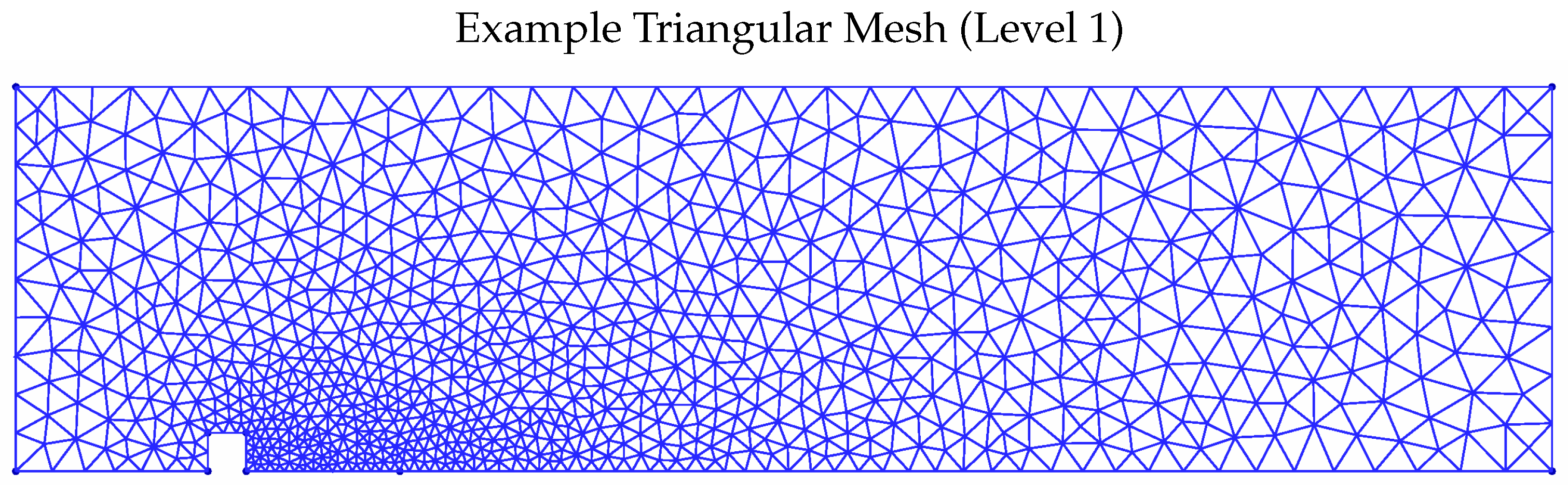
The mesh discretization levels are enumerated in Table 1. An example discretization of the domain can be seen in Figure 1. These meshes were used consistently in [7] and [11]. The “coarse” mesh in [9] is essentially the same as the level-2 mesh, whereas the “fine” mesh has a tighter discretization than the level-3 mesh. Levels 0 and 1 substantially under-resolve the flow in the unregularized NSE in these settings. It is the goal of any regularization model to improve on the performance of these results.

Table 1. These four meshes are utilized consistently in [7,11]. The $N_{dof}$ are calculated for the $(P_3,P_2)$ Taylor–Hood finite elements.

Mesh Scale	${\mathit{N}}_{\mathbf{dof}}$
Level 0	2072
Level 1	5433
Level 2	13,899
Level 3	41,502

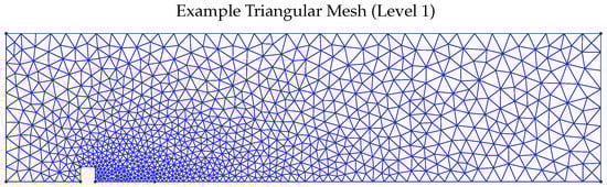
Figure 1. Typically, a tighter discretization is used behind the block to resolve flow rotations.

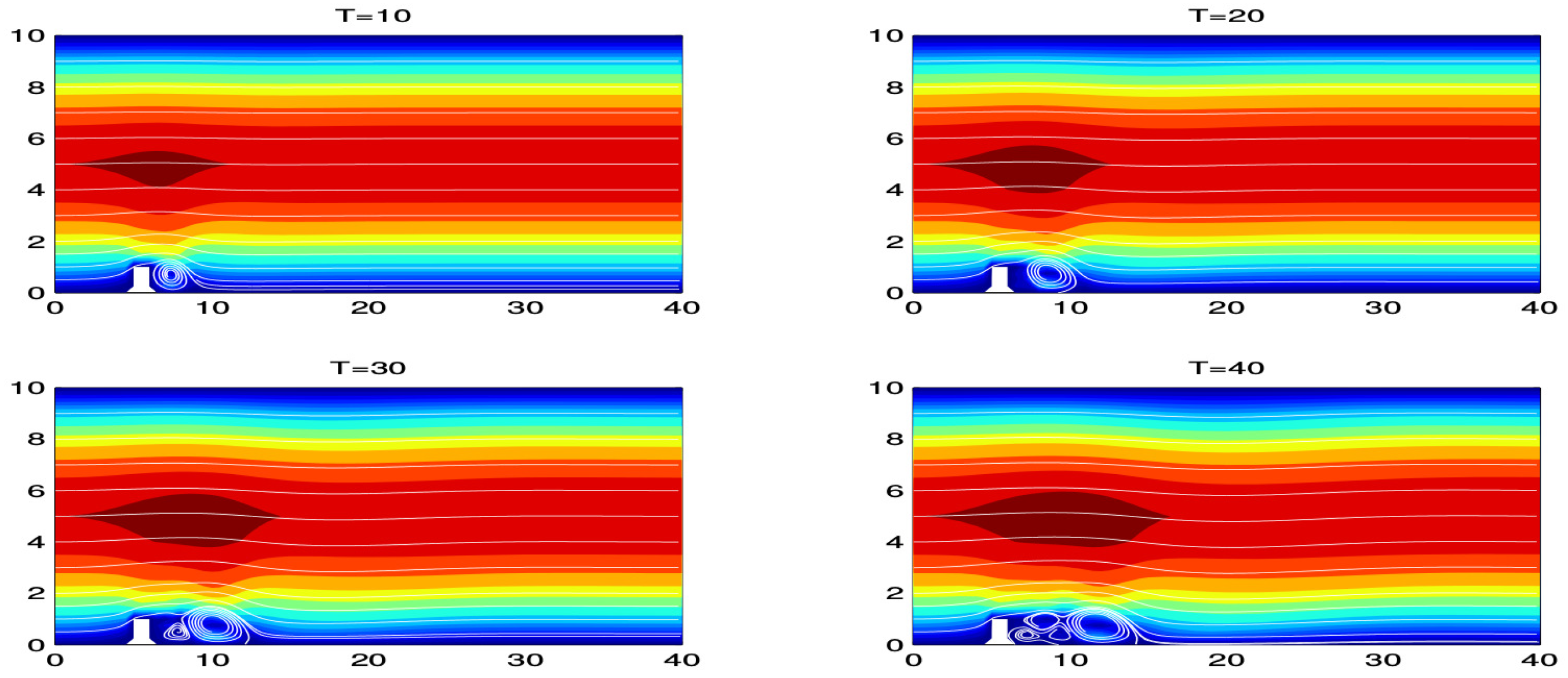
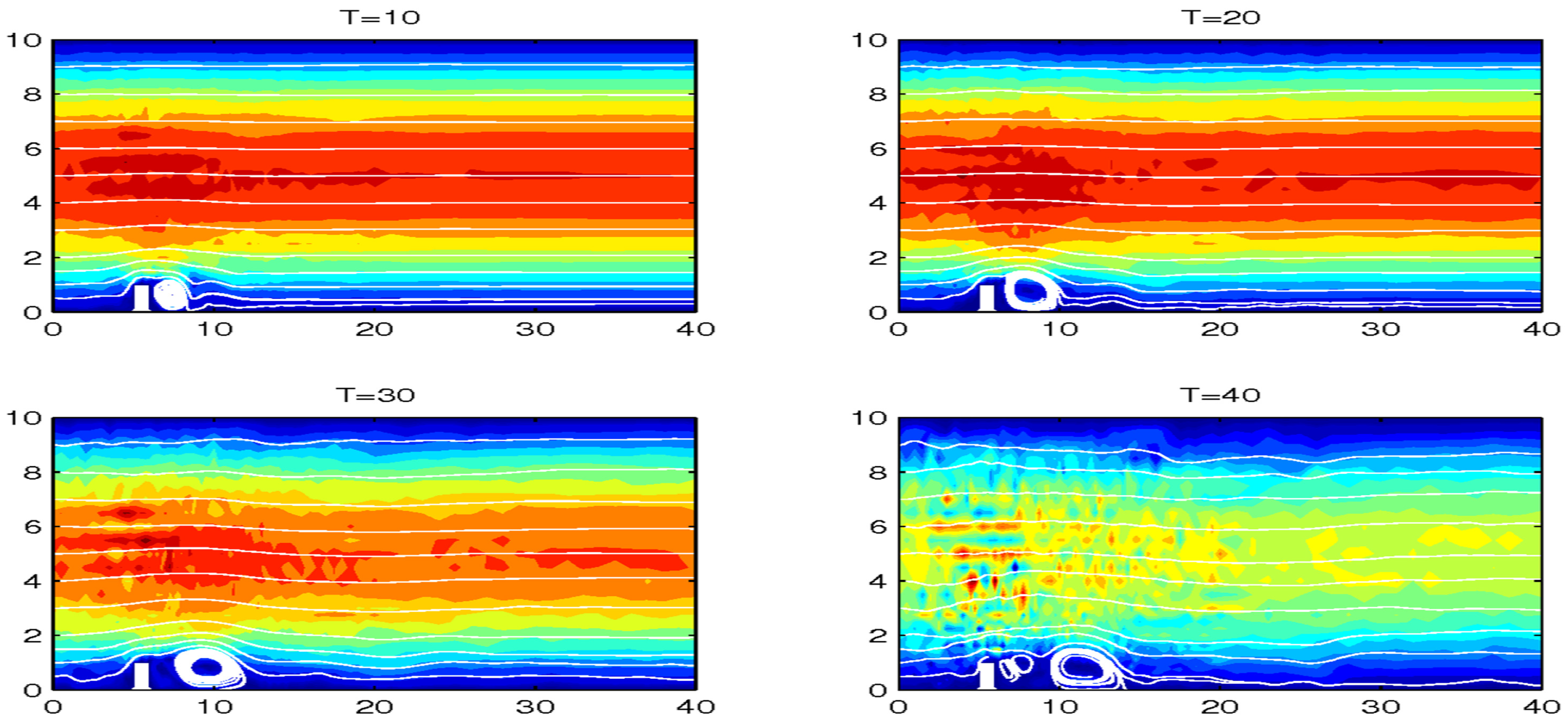
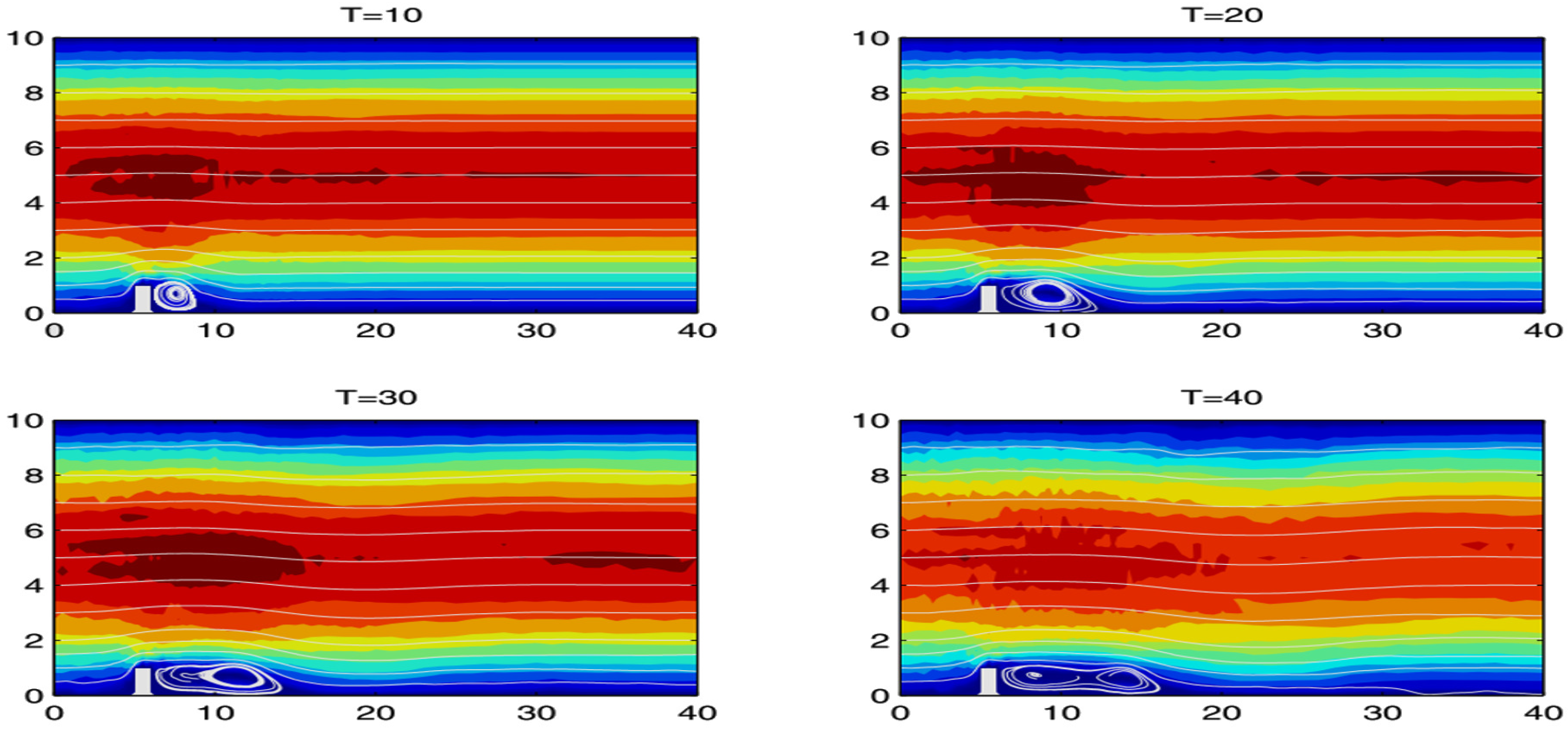
The true behavior is characterized by a vortex growing behind the obstruction, eventually splitting and shedding through time. Typically, the experiment is conducted over the time interval $0\le t\le 40$. An example “correct” solution can be seen at t = 40 s in Figure 2. Contrast this with the under-resolved flow seen Figure 3, where while we still see growing and separating spatial eddies, strong erroneous oscillating features begin to destroy the calculation as time advances. These figures are reported in [11].

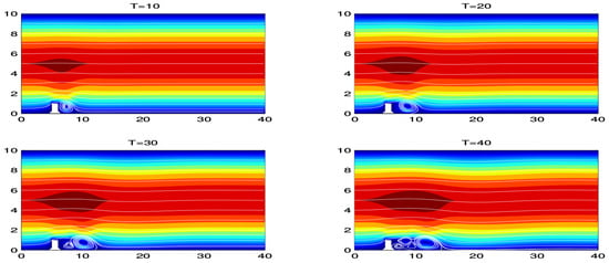
Figure 2. Four snapshots ($t=10, 20, 30,$ and 40) of a full-resolution direct numerical simulation of the Navier–Stokes Equations (NSE). Shown are streamlines overlaid above speed contours $|{\mathbf{v}}_h(\mathbf{x}, t)|$. This figure was originally published in [11].

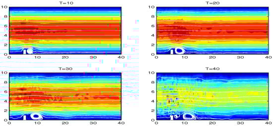
Figure 3. Four snapshots ($t=10, 20, 30,$ and 40) of an under-resolved direct numerical simulation of the NSE, plagued with spurious oscillations. Shown are streamlines overlaid above speed contours $|{\mathbf{v}}_h(\mathbf{x}, t)|$. This figure was originally published in [11].

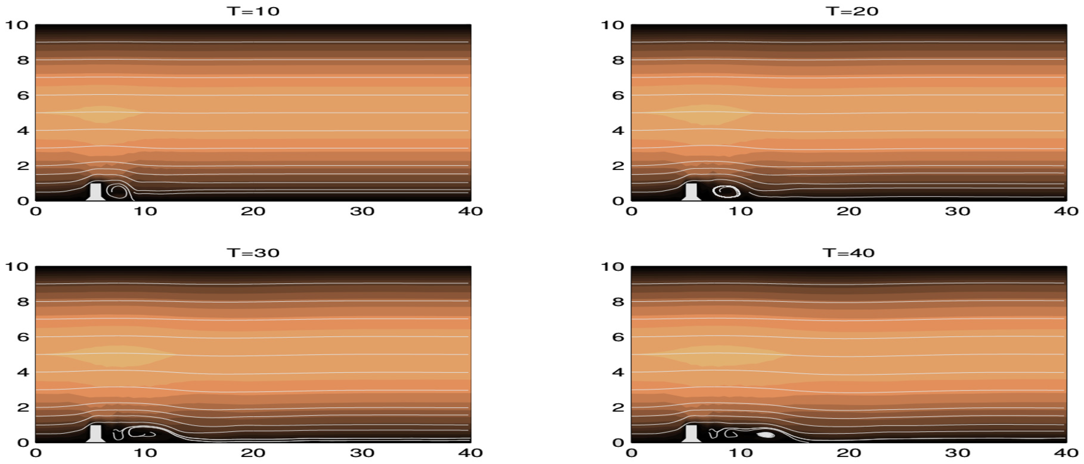
On a level-1 mesh, the linear time relaxation model (9) and (10), with deconvolution order $N=0$, relaxation term $\chi =0.01$, and differential filtering length $\delta =1.5$ shows a considerable improvement over the unregularized NSE. No erroneous speed oscillations are observed, and vortices are seen to be growing and separating. This is seen in Figure 4. Note that Figure 4 comes from [7], where they used a different color-map for the speed contours. It is also worth mentioning that this result comes from the simplest formulation of the considered time relaxation models, paired with well-selected parameter values. Increasing the order of deconvolution to $N=1$ produces a nearly indistinguishable result (which also can be seen in [7]).

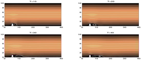
Figure 4. Four snapshots ($t=10, 20, 30,$ and 40) of the linear time relaxation model (TRM) with deconvolution order $N=0$, filter length $\delta =1.5$, and relaxation term $\chi =0.01$. Shown are streamlines overlaid above speed contours $|{\mathbf{v}}_h(\mathbf{x},t)|$. Lighter shades represent higher speeds. This figure was originally published in [7].

As mentioned briefly at the end of Section 3.3, if the relaxation term is increased (be it by a high degree of disagreement measured in the $\left({\mathbf{v}}_h-D_N^h{\overline{\mathbf{v}}}_h\right)$ term, or by substantially increasing $\chi$) the energy dissipation penalty increases proportionally. If the dissipation penalty is too high, the flow can over-regulate. This is observed in [11], where they utilize a nonlinear formulation of the form (26) with $r=3$ (quadratic). On a level-1 mesh, with deconvolution order $N=0$, filtering length $\delta =0.5$, and $\chi =3.0$, we see in Figure 5 that the smaller-scale fluctuations have been over-smoothed such that the vortices will not separate. Increasing to a first-order deconvolution ($N=1$) effectively decreases the dissipation rate, allowing for some of the smaller rotations to be resolved. This growth and splitting can be observed in Figure 6. In both Figure 5 and Figure 6 we see erroneous oscillations growing in time within the speed contours. To address this, one would could increase the filter length $\delta$.

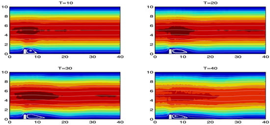
Figure 5. Four snapshots ($t=10, 20, 30,$ and 40) of the nonlinear TRM with deconvolution order $N=0$, filter length $\delta =0.5$, and relaxation term $\chi =3.0$. Shown are streamlines overlaid above speed contours $|{\mathbf{v}}_h(\mathbf{x},t)|$. This figure was originally published in [11].

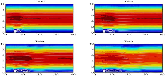
Figure 6. Four snapshots ($t=10,20,30,$ and 40) of the nonlinear TRM with deconvolution order $N=1$, filter length $\delta =0.5$, and relaxation term $\chi =3.0$. Shown are streamlines overlaid above speed contours $|{\mathbf{v}}_h(\mathbf{x},t)|$. This figure was originally published in [11].

4.2. 3D Ethier-Steinman Problem for the Nonlinear Time Relaxation

This numerical computation was performed in [11]. The velocity and pressure of the Eithier–Steinman problem satisfy Navier–Stokes equations exactly. The domain is ${[-1,1]}^3$ and for given parameters $a,d$ and viscosity $\nu$, the solution is given by,

$$\begin{array}{ccc}\hfill u_1& =& -a\left(e^{ax}sin(ay+dz)+e^{az}cos(ax+dy)\right)e^{-\nu d^{2}t}\hfill \end{array}$$

(32)

$$\begin{array}{ccc}\hfill u_2& =& -a\left(e^{ay}sin(az+dx)+e^{ax}cos(ay+dz)\right)e^{-\nu d^{2}t}\hfill \end{array}$$

(33)

$$\begin{array}{ccc}\hfill u_3& =& -a\left(e^{az}sin(ax+dy)+e^{ay}cos(az+dx)\right)e^{-\nu d^{2}t}\hfill \end{array}$$

(34)

$$\begin{array}{ccc}\hfill p& =& -\frac{a^2}{2}(e^{2ax}+e^{2ay}+e^{2az}+2sin(ax+dy)cos(az+dx)e^{a(y+z)}\hfill \\ \hfill & & +2sin(ay+dz)cos(ax+dy)e^{a(z+x)}\hfill \\ \hfill & & +2sin(az+dx)cos(ay+dz)e^{a(x+y)})e^{-\nu d^{2}t}\hfill \end{array}$$

(35)

The parameter values were selected such that $a=1.25$, $d=1$, kinematic viscosity $\nu =0.0001$, time-step $\Delta t=0.005$, final time $T=1$, time relaxation parameter $\chi =1$, and order of deconvolution $N=0$ (for both linear and nonlinear cases). The initial velocity is given by the above true solution, i.e., ${\mathbf{u}}_0={(u_1\left(0\right),u_2\left(0\right),u_3\left(0\right))}^T$. Dirichlet boundary conditions were similarly enforced, given (32)–(34). The mesh considered contained 3072 tetrahedral elements. The finite element discretization used the $(P_2,P_1)$ Taylor–Hood finite elements.

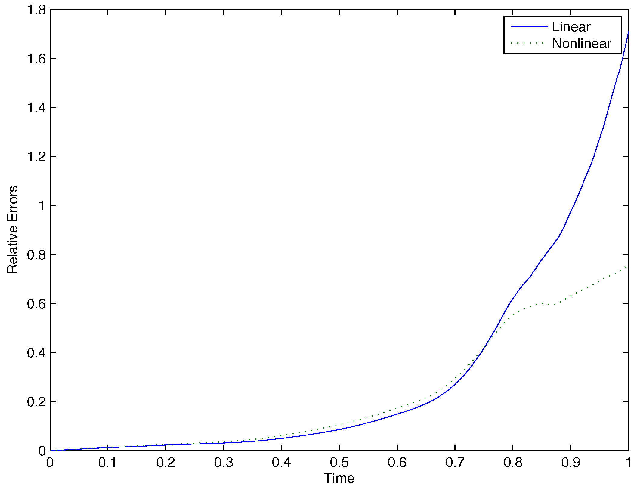
Figure 7 presents graphs of the velocity errors for the linear (full line) and nonlinear (dotted line) time relaxation model in time. The graphs show that the nonlinear relaxation method develops less error as time progresses in time.

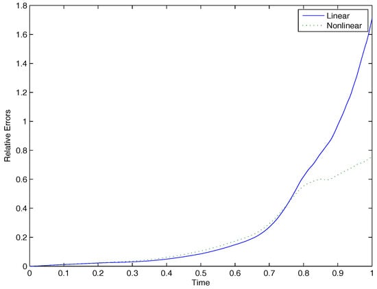
Figure 7. Comparison of the relative $L^2$ error.

4.3. Two-Dimensional Flow about a Cylinder Problem

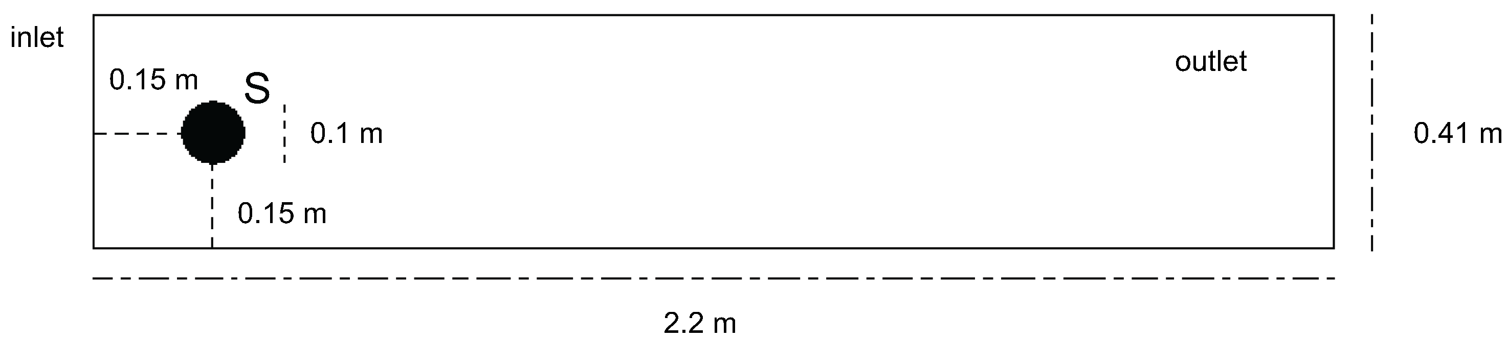
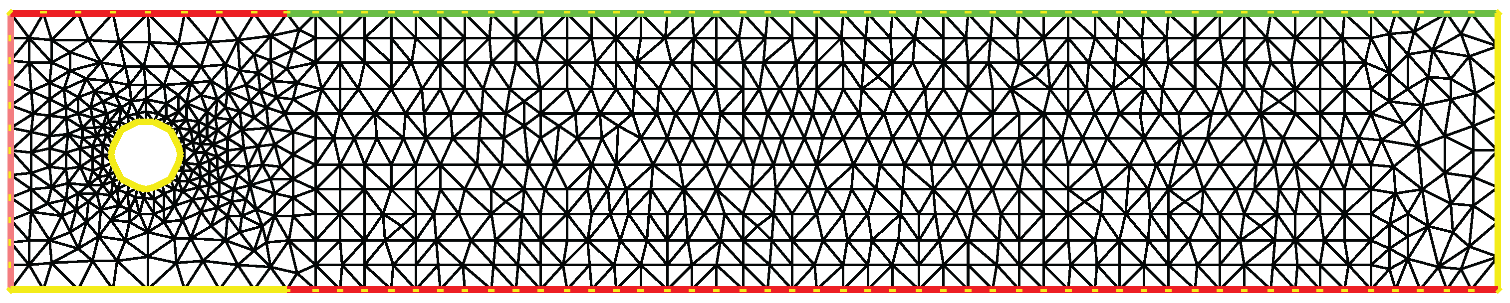
In this study from [10] the creation of the vortex street and calculation of maximum drag and lift, and the change in pressure for a body of rotational form immersed in a fluid was studied. These calculations require accurate estimation of pressure and derivatives of velocity on the flow boundary, which is more difficult than accurately predicting fluid flow velocity. This numerical experiment has been studied by Schafer and Turek in [21] and John in [18]. The domain for the flow is given in Figure 8. The inflow is specified as ${0.41}^{-2}·sin(\pi t/8)·6y(0.41-y)$ m/s, “do-nothing” at the outflow boundary and no slip boundary conditions at the top and bottom of the domain and around the cylinder. Since the mean inflow velocity $U\left(t\right)=sin(\pi t/8)$ ranges from 0 to 1, the Reynolds number $Re=\frac{LU}{\nu }\in [0,\frac{L}{\nu }]=[0, 100]$ as the diameter $L=0.1$ m. The meshes were generated using Delaunay triangulation and three mesh levels are used in simulation: level 1 with 7500 dof, level 2 with 28,806 dof, and level 3 with 114,042 dof. Mesh level 1 is shown in Figure 9. The Taylor–Hood elements are used for space discretization. More details can be found in [10].

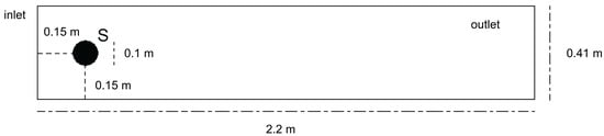
Figure 8. Domain.

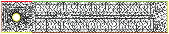
Figure 9. Mesh Level 1.

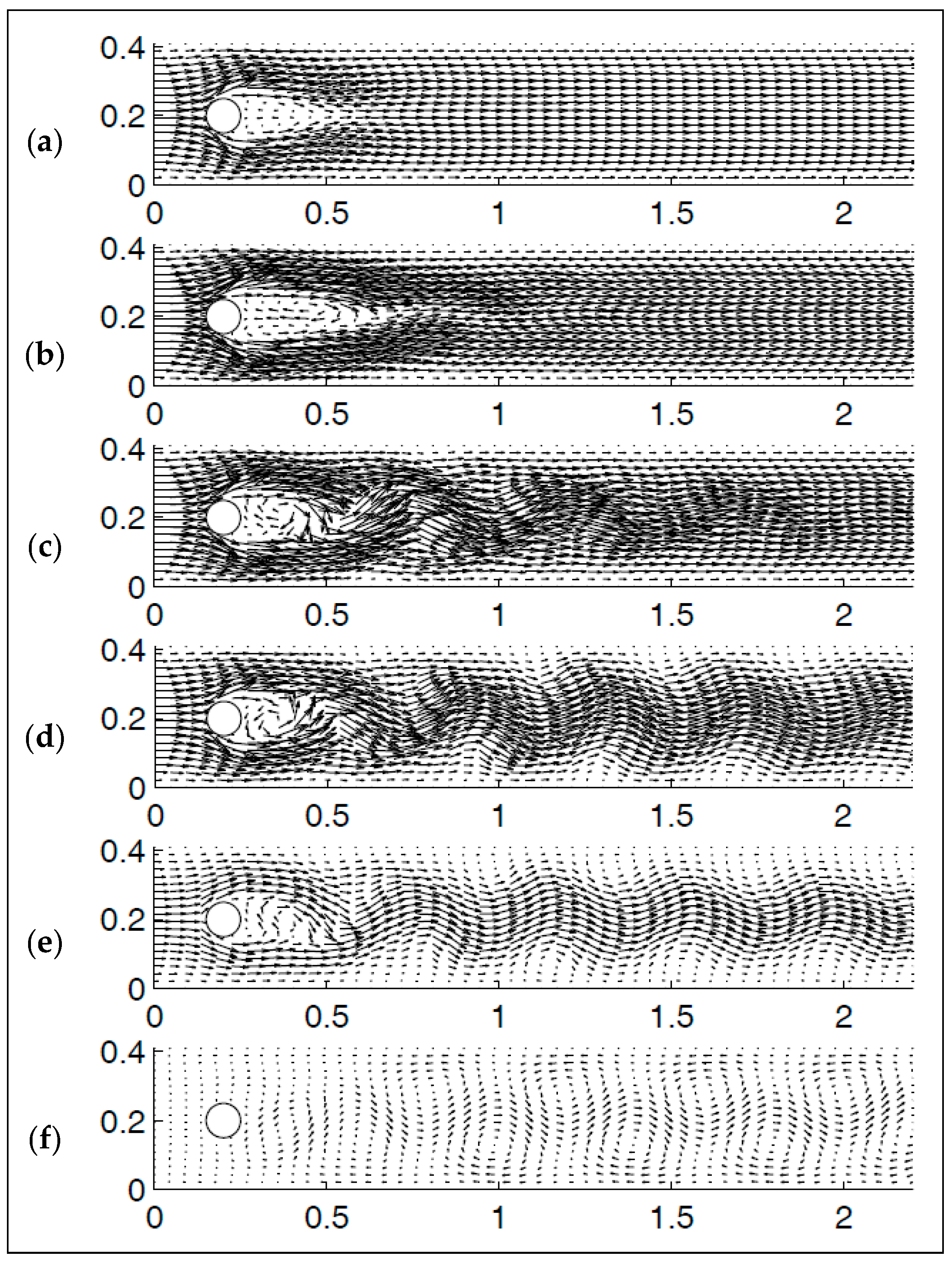
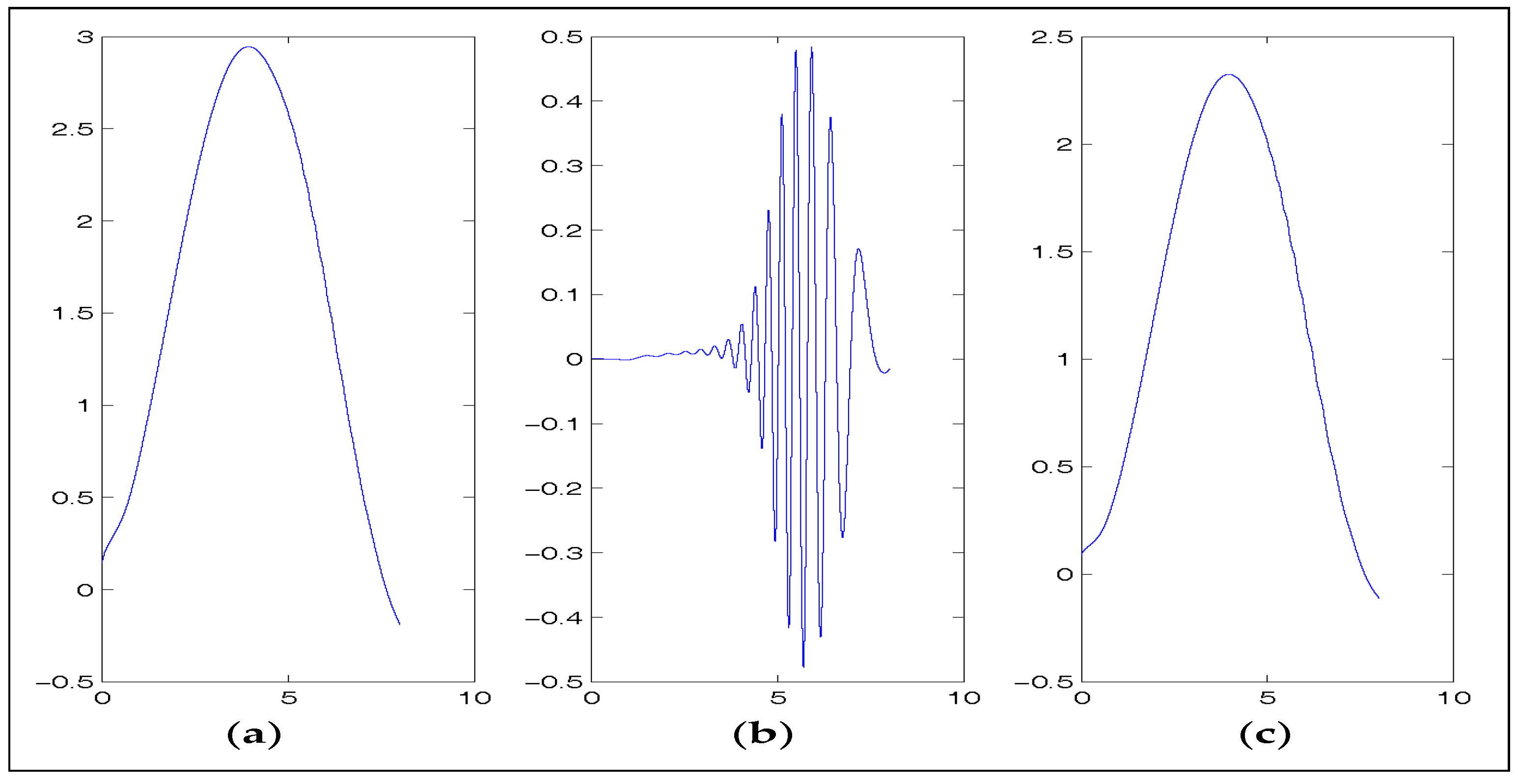
The indication of a successful simulation is the formation of a vortex street, as seen in Figure 10, and the correct profiles in time for drag $c_d\left(t\right)$, lift $c_l\left(t\right)$, and pressure drop $\Delta p\left(t\right)$ may be found in Figure 11.

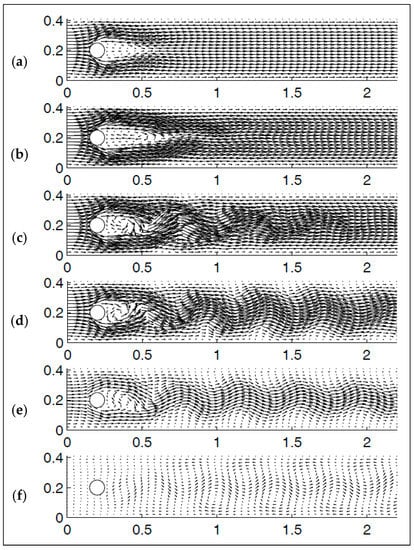
Figure 10. Velocity snapshots presented from (a–f) at t = 2, 4, 5, 6, 7, and 8 for level-3 mesh with $▵t=0.00125$, viscosity $\nu ={10}^{-3}$, $\chi =0.01$ and $N=0$.

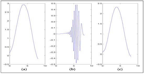
Figure 11. The development of $c_d\left(t\right)$, $c_l\left(t\right)$, and $\Delta p\left(t\right)$ (from to (a–c), respectively) for level-3 mesh with $▵t=0.00125$, viscosity $\nu ={10}^{-3}$, $\chi =0.01$ and $N=0$.

The following reference values are given by John in [18]:

$$\begin{array}{c}t(c_{d,max}^{ref})=3.93625,c_{d,max}^{ref}=2.950921575\hfill \\ t(c_{l,max}^{ref})=5.693125,c_{l,max}^{ref}=0.47795\hfill \\ \Delta p^{ref}(8s)=-0.1116\hfill \end{array}$$

Furthermore, Schäfer and Turek have provided the following reference intervals of:

$$c_{d,max}^{ref}\in [2.93, 2.97],c_{l,max}^{ref}\in [0.47, 0.49], and ▵p^{ref}\left(8s\right)\in [-0.115, -0.105]$$

for the maximum drag, lift, and difference in pressure, respectively [21]. The results of this experiment fall within these reference values on mesh levels 2 and 3 for all the tested time steps, (see Table 2 for order of deconvolution $N=0$).

Table 2. Maximal drag, maximal lift, and change in pressure, order of deconvolution $N=0$.

Level	$▵\mathit{t}$	t (${\mathit{c}}_{\mathit{d},\mathit{max}}$)	${\mathit{c}}_{\mathit{d},\mathit{max}}$	t (${\mathit{c}}_{\mathit{l},\mathit{max}}$)	${\mathit{c}}_{\mathit{l},\mathit{max}}$	$\mathit{\alpha }\mathit{p}$ (8 s)
1	0.04	3.96	2.85876	6.36	0.242883	−0.100637
1	0.02	3.94	2.86052	6.18	0.293106	−0.109724
1	0.01	3.93	2.86136	6.13	0.305785	−0.109681
1	0.005	3.93	2.86177	6.12	0.308338	−0.108987
1	0.0025	3.9275	2.86197	6.115	0.308694	−0.108891
1	0.00125	3.925	2.86208	6.11375	0.308617	−0.108924
2	0.04	3.96	2.94203	6.12	0.393238	−0.10326
2	0.02	3.96	2.94399	5.98	0.464875	−0.105554
2	0.01	3.94	2.94497	5.94	0.477624	−0.110691
2	0.005	3.94	2.94544	5.925	0.48004	−0.111333
2	0.0025	3.9375	2.94567	5.92	0.479669	−0.111552
2	0.00125	3.9375	2.94578	5.91875	0.479152	−0.111665
3	0.04	3.96	2.94543	6.12	0.40593	−0.102126
3	0.02	3.96	2.94741	5.98	0.468239	−0.106822
3	0.01	3.94	2.9484	5.93	0.485103	−0.110926
3	0.005	3.94	2.94887	5.915	0.486785	−0.111227
3	0.0025	3.9375	2.94909	5.9125	0.486471	−0.111363
3	0.00125	3.9375	2.9492	5.9125	0.485944	−0.111455

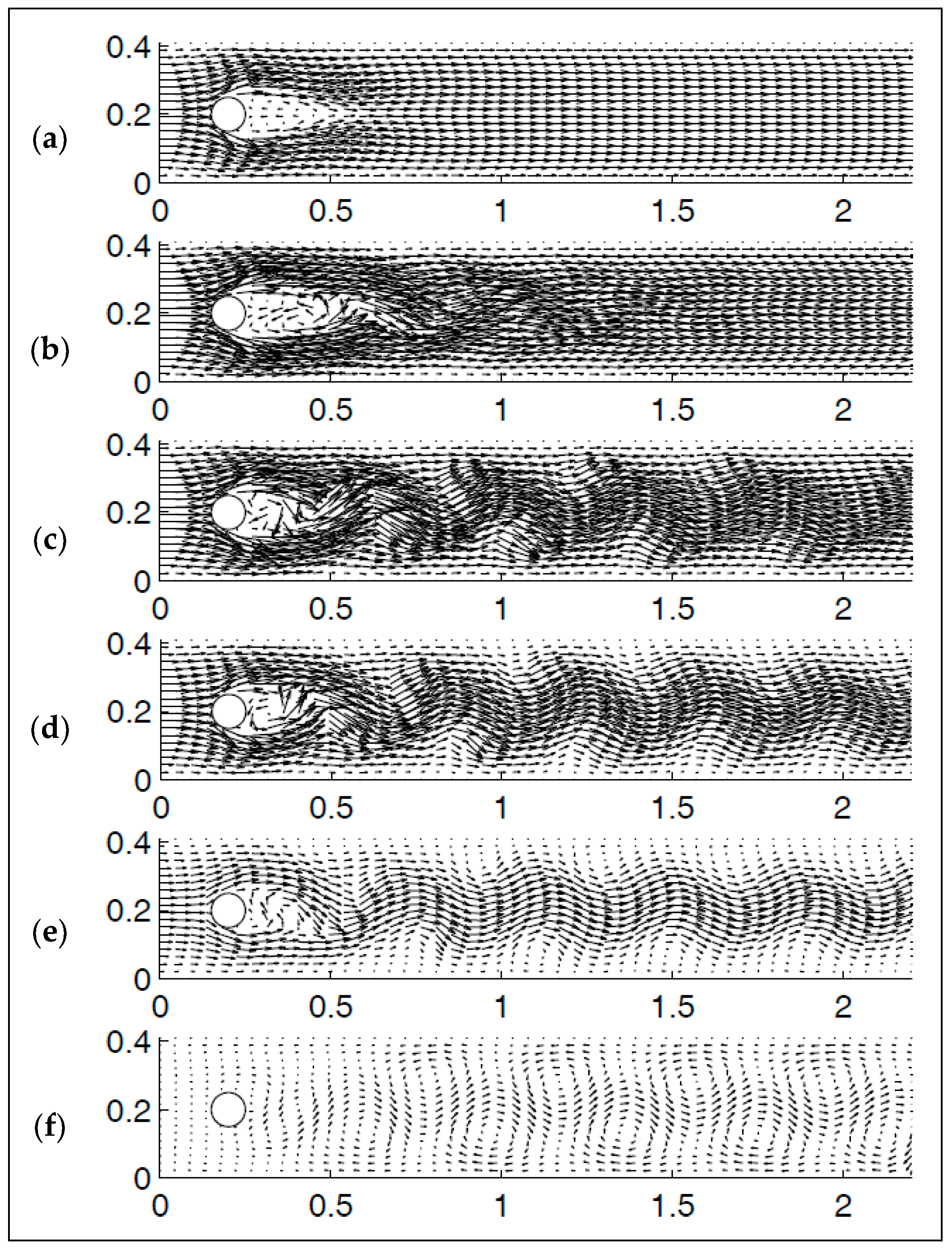
The usefulness of the time relaxation model at higher Reynolds numbers was tested. With $\nu ={10}^{-5}$, a value of $\chi =20$ produced a solution with visible vortex street (see Figure 12), while the Navier–Stokes simulations were unsuccessful (i.e., the fixed point iteration of the nonlinearity did not converge).

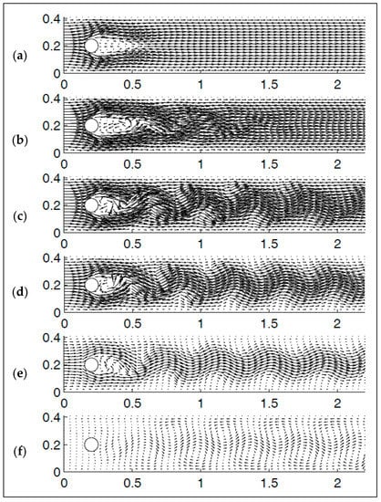
Figure 12. Velocity snapshots presented from (a–f) at t = 2, 4, 5, 6, 7, and 8 for level-2 mesh with $▵t=0.00125$, viscosity $\nu ={10}^{-5}$, $\chi =20$, and $N=0$.

5. Parameter-Sensitivity Study of the Time Relaxation Model

The “optimal” parameter choices for non-physical quantities like the relaxation coefficient $\chi$, nonlinear time relaxation order r, and the filtering length $\delta$ are discussed [6,11,19]. That said, the notion of “optimal” scales for such parameters are inherently problem- and goal-specific. This is further complicated by the fact computed solutions are inherently sensitive to these parameters.

The notion of $\chi —$sensitivity for the linear time relaxation model was addressed in [22]. Since it is understood that a velocity solution $\mathbf{v}$ to the linear model is sensitive to perturbations of $\chi$, we denote velocity solutions to the linear TRM for a given $\chi$ as $\mathbf{v}\left(\chi \right).$ The $\chi =0$ solution results in a direct numerical simulation of the NSE. We can estimate $\chi —$sensitivity by the forward finite difference (FFD)

$${\mathbf{s}}_{FFD}\left(\chi \right)=\frac{\mathbf{v}\left(\chi \right)-\mathbf{v}\left(0\right)}{\chi }.$$

(36)

Further, if we assume $\mathbf{v}\left(\chi \right)$ varies smoothly with $\chi$, we can define the sensitivity as the implicit derivative,

$${\mathbf{s}}_{SEM}\left(\chi \right)=\frac{\partial }{\partial \chi }\mathbf{v}\left(\chi \right).$$

(37)

We similarly define the sensitivity of pressure as $\psi \left(\chi \right)$, and filtered velocity $\mathbf{w}\left(\chi \right)$.

The $\chi —$sensitivity is evaluated in two ways. Firstly, the FFD method (36) can be used and secondly, the sensitivity equation method (SEM) can also be used. The SEM is developed by taking an implicit derivative of (9) and (10), as well a the filter Equation (5). For simplicity, we let ${\mathbf{s}}_{SEM}=\mathbf{s}$ then by selecting $N=0$, the $\chi —$sensitivity equations are written:

$$\begin{array}{ccc}\hfill {\mathbf{s}}_t+\mathbf{v}·\nabla \mathbf{s}+\mathbf{s}·\nabla \mathbf{v}+\nabla \psi -\nu ▵\mathbf{s}+(\mathbf{v}-\overline{\mathbf{v}})+\chi (\mathbf{s}-\mathbf{w})& =& \mathbf{0},\hfill \end{array}$$

(38)

$$\begin{array}{ccc}\hfill \nabla ·\mathbf{s}& =& 0\hfill \end{array}$$

(39)

$$\begin{array}{ccc}\hfill -{\delta }^2▵\mathbf{w}+\mathbf{w}& =& \mathbf{s}.\hfill \end{array}$$

(40)

Initial and boundary conditions for (9) and (10) are inherently insensitive to $\chi$, hence for all implementations,

$$\begin{array}{ccc}\hfill \mathbf{s}(\mathbf{x},0)& =& \mathbf{0},\hfill \\ \hfill \mathbf{s}(\partial \mathrm{\Omega },t)& =& \mathbf{0}.\hfill \end{array}$$

The new PDE (38)–(40) is discretized and computed in conjunction with the model’s discretization. In [22] the SEM equations are discretized using the same scheme, Taylor–Hood $(P_n,P_{n-1})$ finite elements, and Crank–Nicolson time stepping. For notational clarity, in the discussion of the Crank–Nicolson temporal discretization, we let $\mathbf{v}\left(t^{n+1/2}\right)=\mathbf{v}((t^{n+1}+t^n)/2)$ for the continuous variable and ${\mathbf{v}}^{n+1/2}=({\mathbf{v}}^{n+1}+{\mathbf{v}}^n)/2$ for both, continuous and discrete variables. Thus, we obtain the following discretized finite element variational formulations.

Given $({\mathbf{X}}_h,Q_h)$, end-time $T>0$, the time step is chosen $▵t<T=M▵t$, find the approximated TRM solution $({\mathbf{v}}_h^{n+1},p_h^{n+1})\in ({\mathbf{X}}_h,Q_h)$, for $n=0,1,2....M-1$ satisfying,

$$\begin{array}{c}\hfill \frac{1}{▵t}({\mathbf{v}}_h^{n+1}-{\mathbf{v}}_h^n,{\mathit{\varphi }}_h)+\nu a({\mathbf{v}}_h^{n+1/2},{\mathit{\varphi }}_h)+b^{*}({\mathbf{v}}_h^{n+1/2},{\mathbf{v}}_h^{n+1/2},{\mathit{\varphi }}_h)-(p_h^{n+1},\nabla ·{\mathit{\varphi }}_h)\\ \hfill +\chi ({\mathbf{v}}_h^{n+1/2}-{{\overline{\mathbf{v}}}_h}^{n+1/2},{\mathit{\varphi }}_h)=({\mathbf{f}}^{n+1/2},{\mathit{\varphi }}_h),\forall {\mathit{\varphi }}_h\in {\mathbf{X}}_h\end{array}$$

(41)

$$\begin{array}{c}\hfill (\nabla ·{\mathbf{v}}_h^{n+1},q_h)=0,\forall q_h\in Q_h\end{array}$$

(42)

$$\begin{array}{c}\hfill {\delta }^2(\nabla {{\overline{\mathbf{v}}}_h}^{n+1},\nabla {\mathit{\varphi }}_h)+({{\overline{\mathbf{v}}}_h}^{n+1},{\mathit{\varphi }}_h)=({\mathbf{v}}_h^{n+1},{\mathit{\varphi }}_h),\forall {\mathit{\varphi }}_h\in {\mathbf{X}}_h\end{array}$$

(43)

and the sensitivity solution $({\mathbf{s}}_h^{n+1},v_h^{n+1})\in ({\mathbf{X}}_h,Q_h)$, for $n=0,1,2....M-1$ satisfying,

$$\begin{array}{c}\hfill \frac{1}{▵t}({\mathbf{s}}_h^{n+1}-{\mathbf{s}}_h^n,{\mathit{\varphi }}_h)+\nu a({\mathbf{s}}_h^{n+1/2},{\mathit{\varphi }}_h)+b^{*}({\mathbf{s}}_h^{n+1/2},{\mathbf{v}}_h^{n+1/2},{\mathit{\varphi }}_h)+b^{*}({\mathbf{v}}_h^{n+1/2},{\mathbf{s}}_h^{n+1/2},{\mathit{\varphi }}_h)\\ \hfill -({\psi }_h^{n+1},\nabla ·{\mathit{\varphi }}_h)+({\mathbf{v}}_h^{n+1/2}-{{\overline{\mathbf{v}}}_h^h}^{n+1/2},{\mathit{\varphi }}_h)+\chi ({\mathbf{s}}_h^{n+1/2}-{\mathbf{u}}_h^{n+1/2},{\mathit{\varphi }}_h)=0,\forall {\mathit{\varphi }}_h\in {\mathbf{X}}_h\end{array}$$

(44)

$$\begin{array}{c}\hfill (\nabla ·{\mathbf{s}}_h^{n+1},q_h)=0,\forall q_h\in Q_h\end{array}$$

(45)

$$\begin{array}{c}\hfill {\delta }^2(\nabla {\mathbf{u}}_h^{n+1},\nabla z_h)+({\mathbf{u}}_h^{n+1},{\mathit{\varphi }}_h)=({\mathbf{s}}_h^{n+1},{\mathit{\varphi }}_h).\forall {\mathit{\varphi }}_h\in {\mathbf{X}}_h\end{array}$$

(46)

Equations (41)–(43) and (44)–(46) can be rewritten equivalently in the space $V^h$ as given below.

Find ${\mathbf{v}}_h^{n+1}\in V^h$, for $n=0, 1, 2....M-1$ satisfying,

$$\begin{array}{c}\hfill \frac{1}{▵t}({\mathbf{v}}_h^{n+1}-{\mathbf{v}}_h^n,{\mathit{\varphi }}_h)+\nu a({\mathbf{v}}_h^{n+1/2},{\mathit{\varphi }}_h)+b^{*}({\mathbf{v}}_h^{n+1/2},{\mathbf{v}}_h^{n+1/2},{\mathit{\varphi }}_h)\\ \hfill +\chi ({\mathbf{v}}_h^{n+1/2}-{{\overline{\mathbf{v}}}_h^h}^{n+1/2},{\mathit{\varphi }}_h)=({\mathbf{f}}^{n+1/2},{\mathit{\varphi }}_h),\forall {\mathit{\varphi }}_h\in V^h\end{array}$$

(47)

$$\begin{array}{c}\hfill {\delta }^2(\nabla {{\overline{\mathbf{v}}}_h^h}^{n+1},\nabla {\mathit{\varphi }}_h)+({{\overline{\mathbf{v}}}_h^h}^{n+1},{\mathit{\varphi }}_h)=({\mathbf{v}}_h^{n+1},{\mathit{\varphi }}_h),\forall {\mathit{\varphi }}_h\in V^h\end{array}$$

(48)

and for the sensitivity solution, find ${\mathbf{s}}_h^{n+1}\in V^h$, for $n=0,1,2....M-1$ satisfying,

$$\begin{array}{c}\hfill \frac{1}{▵t}({\mathbf{s}}_h^{n+1}-{\mathbf{s}}_h^n,{\mathit{\varphi }}_h)+\nu a({\mathbf{s}}_h^{n+1/2},{\mathit{\varphi }}_h)+b^{*}({\mathbf{s}}_h^{n+1/2},{\mathbf{v}}_h^{n+1/2},{\mathit{\varphi }}_h)+b^{*}({\mathbf{v}}_h^{n+1/2},{\mathbf{s}}_h^{n+1/2},{\mathit{\varphi }}_h)\\ \hfill +({\mathbf{v}}_h^{n+1/2}-{{\overline{\mathbf{v}}}_h^h}^{n+1/2},{\mathit{\varphi }}_h)+\chi ({\mathbf{s}}_h^{n+1/2}-{\mathbf{u}}_h^{n+1/2},{\mathit{\varphi }}_h)=0,\forall {\mathit{\varphi }}_h\in V^h\end{array}$$

(49)

$$\begin{array}{c}\hfill {\delta }^2(\nabla {\mathbf{u}}_h^{n+1},\nabla {\mathit{\varphi }}_h)+({\mathbf{u}}_h^{n+1},{\mathit{\varphi }}_h)=({\mathbf{s}}_h^{n+1},{\mathit{\varphi }}_h),\forall {\mathit{\varphi }}_h\in V^h\end{array}$$

(50)

The $\chi —$sensitivity is evaluated on several benchmark problems that consider a variety of mesh scales and Reynolds numbers. Each sensitivity calculation is computed by both the FFD and SEM techniques. One such benchmark is the 2D lid-driven cavity problem where $\mathrm{\Omega }={[0, 1]}^2$, and $0\le t\le 1.0$. The initial and boundary conditions for the linear TRM velocity are given by,

$$\begin{array}{ccc}\hfill \mathbf{v}(\mathbf{x},t)& =& {(16x^2{(1-x)}^2,0)}^T,\mathbf{x}\in \partial \mathrm{\Omega }\cap \{y=1\},\hfill \\ \hfill \mathbf{v}(\mathbf{x},t)& =& \mathbf{0},\mathbf{x}\in \partial \mathrm{\Omega }\cap \{y<1\},\hfill \\ \hfill \mathbf{v}(\mathbf{x},0)& =& {(3y^2-2y,0)}^T.\hfill \end{array}$$

The $\chi —$sensitivity estimates are enumerated in Table 3 and Table 4. It is with these values that one can determine the reliability of a the linear time relaxation model when $\chi \in [0.1, 10.0]$.

Table 3. Computations of $\chi {\left|\left|{\mathbf{s}}_{SEM}\right|\right|}_{L^2([0,1];L^2\left(\mathrm{\Omega }\right))}$ for the lid-driven cavity problem.

$\mathit{\chi }$	$\mathit{Re}=$ 1000	$\mathit{Re}=$ 5000	$\mathit{Re}=$ 10,000
0.01	$1.068$×${10}^{-4}$	$1.913$×${10}^{-4}$	$2.248$×${10}^{-4}$
0.1	$1.036$×${10}^{-3}$	$1.840$×${10}^{-3}$	$2.155$×${10}^{-3}$
1.0	$8.033$×${10}^{-3}$	$1.314$×${10}^{-2}$	$1.493$×${10}^{-2}$
10.0	$5.038$×${10}^{-2}$	$6.006$×${10}^{-2}$	$6.215$×${10}^{-2}$

Table 4. Computations of $\chi {\left|\left|{\mathbf{s}}_{FFD}\right|\right|}_{L^2([0, 1];L^2\left(\mathrm{\Omega }\right))}$ for the lid-driven cavity problem.

$\mathit{\chi }$	$\mathit{Re}=$ 1000	$\mathit{Re}=$ 5000	$\mathit{Re}=$ 10,000
0.01	$1.075$×${10}^{-4}$	$1.996$×${10}^{-4}$	$2.402$×${10}^{-4}$
0.1	$1.056$×${10}^{-3}$	$1.935$×${10}^{-3}$	$2.317$×${10}^{-3}$
1.0	$8.994$×${10}^{-3}$	$1.466$×${10}^{-2}$	$1.675$×${10}^{-2}$
10.0	$3.173$×${10}^{-2}$	$3.650$×${10}^{-2}$	$3.734$×${10}^{-2}$

5.1. Comparing the SEM and FFD Methods

In [22], the authors used both the SEM and FFD techniques, under the assumption they would provide similar results in the tested settings. This appears to have been done as a form of sanity check. Neither technique demonstrates an overall advantage. For instance, both methods require effectively doubling all computational efforts by solving a second system of equations. Both methods are also easily implemented in working code bases.

The only situation that would necessitate the use of FFD over the SEM is if there is good reason to doubt the existence of the implicit derivatives in (37). On the other hand, a FFD computation is effectively meaningless if the $\mathbf{v}(\chi =0)$ case is unstable or otherwise unreliable, which is not uncommon in under-resolved flows at higher Reynolds numbers. The choice of implementing one technique over the other is largely problem-specific, and a question best left to the good judgment of future authors.

5.2. Determining Reliability of Time-Relaxation Models $\chi$ through Sensitivity Study

As mentioned at the beginning of this section, determining an optimal choice of $\chi$ is a difficult endeavor. Sensitivity studies can be used with great effect to help quantify the reliability of such calculations. While [22] did not explore particular methods to directly quantify model reliability, examples can be found in [23,24]. One such technique is to quantify reliability by using the linear estimate,

$$\left|\right|{\mathbf{v}}_h\left(0\right)-{\mathbf{v}}_h\left(\chi \right)\left|\right|\le \chi \left|\right|{\mathbf{s}}_h\left|\right|+\mathcal{O}\left({\chi }^2\right).$$

(51)

The above estimate holds for any norm.

If, for example, the total kinetic energy of a particular flow is known or can be accurately estimated, enforcing a $\%—$accuracy as an upper bound can determine permissible intervals of model-reliability. Likewise, if for a given norm, the goal is for the computed results of the TRM model to be accurate to within 5% of $\left|\right|{\mathbf{u}}_{true}\left|\right|$, we simply attempt to find an interval $0<a\le \chi \le b$ such that,

$$\begin{array}{}\chi \left|\right|{\mathbf{s}}_h\left|\right|\le 0.05\left|\right|{\mathbf{u}}_{true}\left|\right|.\end{array}$$

(52)

To date, this type of study has not been performed on time relaxation models, and would make for interesting future work.

6. Conclusions and Open Problems

Herein we have presented a summary of a selection of published results about and relevant to time relaxation models. We briefly introduced the technique and the motivations for their development, as well as the results from several computational implementations. While numerous studies have been performed in literature, a number of open questions remain.

Much of the numerical results surveyed herein use the Crank–Nicolson time-stepping scheme. The behavior of linear and nonlinear TRMs with alternate time-stepping schemes, like BDF2 or schemes that permit a variable time-step, remains an open problem. Higher-order time-stepping schemes have also not been considered.

It would be interesting to see the extent to which the energy dissipation penalty for the nonlinear TRM parameter, as determined by $\chi$ and r, affects the energy cascade. Furthermore, numerical experiments have not been seen for nonlinear orders greater than the quadratic case, $r>3$.

In fluid flow problems, approximate deconvolution has been largely accomplished by the van Cittert approximate deconvolution technique. Other techniques exist, i.e. Guerts approximate inverse operators [25], and others. Time relaxation models would be an excellent test bed for such studies, given their simplicity.

So far, the only parameter sensitivity investigation for TRMs was performed in [22], wherein analysis and experiments to estimate $\chi —$sensitivity were done. It would be interesting to see a full analysis of the $\delta ,r,$ and $\chi$ sensitivities for both the linear and nonlinear TRMs. It would also be interesting to see how these parameters affect the outcomes of important functionals, i.e. forces acting on submerged bodies like lift and drag, or physical quantities like energy, enstrophy, helicity, and their dissipations. Finally, a full investigation into the reliability of time relaxation models in challenging computational settings would be of particular interest. This is briefly discussed in Section 5.2.

References

- Kistler, R. A Study of Data Assimilation Techniques in an Autobarotropic Primitive Equation Channel Model. Master’s Thesis, Penn State University, State College, PA, USA, 1974. [Google Scholar]
- Hoke, J.; Anthes, R. The initialization of numerical models by a dynamic-initialization technique. Mon. Weather Rev. 1976, 104, 1551–1556. [Google Scholar] [CrossRef]
- Kolmogorov, A. The local structure of turbulence in incompressible viscous fluids for very large Reynolds numbers. Dokl. Akad. Nauk SSR 1941, 30, 9–13. [Google Scholar] [CrossRef]
- Stolz, S.; Adams, N.; Kleiser, L. The approximate deconvolution model for large-eddy simulations of compressible flows and its application to shock-turbulent-boundary-layer interaction. Phys. Fluids 2001, 13, 2985–3001. [Google Scholar] [CrossRef]
- Stolz, S.; Adams, N.; Kleiser, L. An approximate deconvolution model for large-eddy simulation with application to incompressible wall-bounded flows. Phys. Fluids 2001, 13, 997–1015. [Google Scholar] [CrossRef]
- Layton, W.; Neda, M. Truncation of scales by time relaxation. J. Math. Anal. Appl. 2007, 325, 788–807. [Google Scholar] [CrossRef]
- Ervin, V.; Layton, W.; Neda, M. Numerical analysis of a higher order time relaxation model of fluids. Int. J. Numer. Anal. Model. 2007, 4, 648–670. [Google Scholar]
- Neda, M. Discontinuous time relaxation method for the time-dependent Navier-Stokes equations. Adv. Numer. Anal. 2010, 2010, 21. [Google Scholar] [CrossRef]
- Neda, M.; Sun, X.; Yu, L. Increasing accuracy and efficiency for regularized Navier-Stokes equations. Acta Appl. Math. 2012, 118, 57–79. [Google Scholar] [CrossRef]
- De, S.; Hannasch, D.; Neda, M.; Nikonova, E. Numerical analysis and computations of a high accuracy time relaxation fluid flow model. Int. J. Comput. Math. 2012, 89, 2353–2373. [Google Scholar] [CrossRef]
- Dunca, A.; Neda, M. Numerical analysis of a nonlinear time relaxation model of fluids. J. Math. Anal. Appl. 2014, 420, 1095–1115. [Google Scholar] [CrossRef]
- Takhirov, A.; Neda, M.; Waters, J. Time relaxation algorithm for flow ensembles. Numer. Methods Partial Differ. Equ. 2016, 32, 757–777. [Google Scholar] [CrossRef]
- Neda, M.; Waters, J. Finite element computations of time relaxation algorithm for flow ensembles. Appl. Eng. Lett. 2016, 1, 51–56. [Google Scholar]
- Germano, M. Differential filters for the large eddy numerical simulation of turbulent flows. Phys. Fluids 1986, 29, 1755–1757. [Google Scholar] [CrossRef]
- Bertero, M.; Boccacci, P. Introduction to Inverse Problems in Imaging; CRC Press: Boca Raton, FL, USA, 1998. [Google Scholar]
- Rosenau, P. Extending hydrodynamics via the regularization of the Chapman–Enskog expansion. Phys. Rev. A 1989, 40, 7193–7196. [Google Scholar] [CrossRef]
- Schochet, S.; Tadmor, E. The regularized Chapman–Enskog expansion for scalar conservation laws. Arch. Ration. Mech. Anal. 1992, 119, 95–107. [Google Scholar] [CrossRef]
- Volker, J. Reference values for drag and lift of a two-dimensional time-dependent flow around a cylinder. Int. J. Numer. Methods Fluids 2004, 44, 777–788. [Google Scholar]
- Connors, J.; Layton, W. On the Accuracy of the Finite Element Method Plus Time Relaxation. Math. Comput. 2010, 79, 619–648. [Google Scholar] [CrossRef]
- Hecht, F. New development in FreeFem++. J. Numer. Math. 2012, 20, 251–265. [Google Scholar] [CrossRef]
- Schäfer, M.; Turek, S. The benchmark problem ‘flow around a cylinder’. In Flow Simulation with High-Performance Computers II, Notes on Numerical Fluid Mechanics; Vieweg + Teubner Verlag: Wiesbaden, Germany, 1996; Volume 52, pp. 547–566. [Google Scholar]
- Neda, M.; Pahlevani, F.; Waters, J. Sensitivity Analysis of the Time Relaxation Model. Appl. Math. Mech. 2015, 7, 89–115. [Google Scholar]
- Pahlevani, F.; Davis, L. Parameter Sensitivity of an Eddy Viscosity Model: Analysis, Computation, and It’s Application to Quantifying Model Reliability. Int. J. Uncertain. Quantif. 2013, 3, 397–419. [Google Scholar] [CrossRef]
- Breckling, S.; Neda, M.; Pahlevani, F. Sensitivity Analyses of the Navier-Stokes-α Model. 2017. submitted. [Google Scholar]
- Geurts, B.J. Inverse modeling for large-eddy simulation. Phys. Fluids 1997, 9, 3585–3587. [Google Scholar] [CrossRef]
© 2017 by the authors. Licensee MDPI, Basel, Switzerland. This article is an open access article distributed under the terms and conditions of the Creative Commons Attribution (CC BY) license (http://creativecommons.org/licenses/by/4.0/).