Dynamics of a Highly Viscous Circular Blob in Homogeneous Porous Media

Abstract

Viscous fingering is ubiquitous in miscible displacements in porous media, in particular, oil recovery, contaminant transport in aquifers, chromatography separation, and geological CO₂ sequestration. The viscosity contrasts between heavy oil and water is several orders of magnitude larger than typical viscosity contrasts considered in the majority of the literature. We use the finite element method (FEM)-based COMSOL Multiphysics simulator to simulate miscible displacements in homogeneous porous media with very large viscosity contrasts. Our numerical model is suitable for a wide range of viscosity contrasts covering chromatographic separation as well as heavy oil recovery. We have successfully captured some interesting and previously unexplored dynamics of miscible blobs with very large viscosity contrasts in homogeneous porous media. We study the effect of viscosity contrast on the spreading and the degree of mixing of the blob. Spreading (variance of transversely averaged concentration) follows the power law $t^{3.34}$ for the blobs with viscosity $\sim \mathcal{O}({10}^2)$ and higher, while degree of mixing is found to vary non-monotonically with log-mobility ratio. Moreover, in the limit of very large viscosity contrast, the circular blob behaves like an erodible solid body and the degree of mixing approaches the viscosity-matched case.

1. Introduction

Displacement of a less mobile fluid by a more mobile one in a porous medium results in a hydrodynamic instability, viscous fingering (VF). Its wide applicabilities, e.g., enhanced oil recovery [1], CO₂ sequestration [2], chromatographic separation [3,4], contaminant transport in aquifers [5], mixing in low-Reynolds number flow [6], intrinsic characteristics of nonlinear dynamics and pattern formation have fascinated active theoretical, numerical [6,7,8,9,10,11,12,13], and experimental [14] researchers for more than half a decade. Both rectilinear and radial displacements have been investigated rigorously and have their own significance that can be investigated independently as well as comparatively. Here, we are interested in rectilinear displacements in porous media. The majority of the studies are focused on the case when the defending fluid is separated from the invading fluid by a flat interface. In many situations, e.g., aquifers, the contaminant can be of an arbitrary shape and miscible to the ambient fluid [15]. When the underlying fluids are miscible to each other, the finger-like patterns that develop at the fluid–fluid interface depend, to a great extent, on the shape of the interface [13], viscosity contrast [1], and diffusion rate [16]. As a consequence, mixing, spreading, and breakthrough time alter greatly [6,13,15]. Pramanik et al. used the Fourier pseudospectral method to capture the dynamics of a more viscous blob in a homogeneous porous medium [13], and the results are summarized in the R-Pe parameter plane. Here, R is the log-mobility ratio and Pe is the Péclet number. Depending upon the blob dynamics, R-Pe plane was demarcated into three regions: lump-, comet-shaped deformations, and VF. Their studies were restricted to $R\le 2.5$, and Pe $\le 2500$, due to the limitations of the numerical convergence of the semi-implicit time integration of the pseudo-spectral method. The novelty of their work was identifying the re-entrance into the comet deformation region for large R and fixed Pe, which is in strong contrast with the planar interface cases.

The dynamic viscosity of heavy oils is several orders magnitude larger than water or the conventional polymer used in polymer flooding oil recovery processes. Severe VF during water flooding of heavy oils leaves a large amount of residual oil in the reservoir [17]. To the best of the authors’ knowledge, only experimental studies are conducted for very large viscosity contrast [17]. This captivates us to numerically analyze miscible displacements, mixing, and spreading with very large viscosity contrasts. Various numerical schemes, e.g., finite difference (FD) [7,18], pseudospectral (PS) [9,11], finite element (FE) [10], compact FD with alternating direction implicit (ADI) [19], hybrid FD-PS [20], finite volume (FV) [6], etc., have been used for the nonlinear simulations of miscible VF. In spite of exhaustive numerical studies, miscible VF for large viscosity-contrast fluids are poorly explored. For large viscosity contrasts, the fluid velocity at the interface has sharp gradients. In these cases, one needs to solve a stiff system [20] that limits the numerical convergence [6]. This can be overcome through a suitable choice of the time-discretization method. Islam and Azaiez reported convergent numerical results for viscosity ratios of $\mathcal{O}\left({10}^3\right)$. For water/polymer flooding of heavy oils, the viscosity ratios can go as high as $\mathcal{O}\left({10}^4\right)$ [17]. We present numerical model using COMSOL Multiphysics software [21] to obtain convergent numerical results for viscosity ratios of $\mathcal{O}\left({10}^6\right)$.

Exploring the dynamics of the blob in the comet deformation region for very large R is one of the motives of the present study. We have shown that for very large viscosity contrasts, variance of the transversely averaged concentration follows a power-law ∼$t^{3.34}$ at later times. This power-law is larger than the one ($t^{2.5}$) for moderate viscosity contrast [13]. The structure of the paper is as follows. The mathematical modeling and the methods used for the solution of the formulated problem are presented in Section 2. In Section 3, we present the results of our numerical experiments, followed by the discussion and conclusions of the results in Section 4.

2. Mathematical Formulation and Numerical Methods of Solutions

2.1. Physical Description of the Problem

We investigate the transport in porous media of a more viscous fluid localized in a circular blob. For the numerical modeling, we consider a rectangular domain $L_x\times L_y$ filled by a less viscous fluid (Fluid I) of viscosity ${\mu }_1$, which surrounds a circular blob of a more viscous fluid (Fluid II) of viscosity ${\mu }_2$ (see Figure 1).

Fluid I is injected from left to right along the increasing x-direction at a constant average velocity U. Fluids are assumed to be incompressible, Newtonian, and non-reactive. This is modeled as a single-phase fluid (water) such that the physical properties (e.g., dynamic viscosity) depend on the local variation of the solute concentration (e.g., mass fraction of glycerol in water), c. Without any loss of generality, we assume $c=0$ in the displacing fluid, $c=1$ in displaced one, and gravity is disregarded in our model. The equations governing this flow are,

$$\overrightarrow{\mathsf{\nabla }}·\overrightarrow{u}=0,$$

(1)

$$\overrightarrow{\mathsf{\nabla }}p=-\frac{\mu \left(c\right)}{\kappa }\overrightarrow{u},$$

(2)

$$ϵ\frac{\partial c}{\partial t}+\left(\overrightarrow{u}·\overrightarrow{\mathsf{\nabla }}\right)c=\overrightarrow{\mathsf{\nabla }}·\left(D\overrightarrow{\mathsf{\nabla }}c\right).$$

(3)

Here, $\overrightarrow{u}=(u,v)$ is the two-dimensional Darcy’s velocity vector, D is the isotropic dispersion coefficient, $\mu$ is the dynamic viscosity of the fluid, $\kappa$ and $ϵ$ are, respectively, the permeability and the porosity of the medium. For simplicity, we assume $\kappa$, $ϵ$ are constants, and D is equal to the molecular diffusion coefficient of the solute in the host fluid. The dependence of $\mu$ on c is taken as [1],

$$\mu \left(c\right)={\mu }_1{e}^{Rc},$$

(4)

where the parameter ${\displaystyle R=ln\left(\frac{{\mu }_2}{{\mu }_1}\right)}$ is called the log-mobility ratio.

2.2. COMSOL Multiphsysics Simulations

We are interested in the dynamics of a highly viscous miscible blob in homogeneous porous media. Numerical simulations are performed using FEM-based commercial software COMSOL Multiphysics 5.2a [21]. We use the “Two-Phase Darcy’s Law” (TPDL) model from the “Fluid Flow” module for the simulations shown in this paper. We begin by explaining why and how “Two-Phase Darcy’s law” of COMSOL Myltiphysics is used in miscible VF simulations. Disregarding gravity and capillary pressure, the model equations for TPDL become,

$$\frac{\partial \rho }{\partial t}+\overrightarrow{\mathsf{\nabla }}·\rho \overrightarrow{u}=0,$$

(5)

$$\overrightarrow{u}=-\frac{\kappa }{\mu }\overrightarrow{\mathsf{\nabla }}p,$$

(6)

$$\frac{\partial \left(ϵc_1\right)}{\partial t}+\overrightarrow{\mathsf{\nabla }}·\left(c_1\overrightarrow{u}\right)=\overrightarrow{\mathsf{\nabla }}·(D_c\overrightarrow{\mathsf{\nabla }}{c}_1),$$

(7)

where $\kappa$ is the permeability, $\overrightarrow{u}$ is the two-dimensional Darcy’s velocity, $ϵ$ is the porosity of the medium and $c_1$ is the species concentration. The resultant mobility is related to the mobility of the fluid phases via ${\displaystyle \frac{\kappa }{\mu }=s_1\frac{\kappa {\kappa }_{r1}}{{\mu }_1}+s_2\frac{\kappa {\kappa }_{r2}}{{\mu }_2}}$, where ${\kappa }_{ri},{\mu }_i,s_i$ are the relative permeability, dynamic viscosity, and saturation of phase-$i,i=1,2$, respectively. Saturation of phase-2 is the complement of the phase-1 saturation, i.e., $s_2=1-s_1$. For constant density, Equations (5)–(7) are of the similar form of Equations (1)–(3). Therefore, suitably choosing the mobility and the other physical parameters (viz. dimensions of domain, injection velocity U, diffusion coefficient, etc.), one recovers the exact model described in Section 2.1. We exploit this mathematical analogy between a two-phase porous media flow with capillary diffusion and a single phase species transport in porous media. In the absence of the capillary pressure, the momentum conservation of both the phases is governed by single Darcy’s law, constrained with the incompressibility condition (divergence-free velocity for constant density), described by Equations (5) and (6). This is coupled with a convection-diffusion equation, Equation (7), which describes the mass conservation of the concentration of phase-1. The convection speed is the fluid velocity derived from the Darcy’s law, and the diffusion coefficient is the capillary diffusion. Furthermore, we assume phase-2 as water and define the species concentration/mass fraction (e.g., glycerol), $c=c_1={\rho }_1(1-s_2)={\rho }_1{s}_1$. Since the gravity is disregarded, the model is independent of the density of phase-1, ${\rho }_1$. Without lost of generality, arbitrary values can be assigned to this. For simplicity, we choose ${\rho }_1$ as unity, and denote $c=s_1$ in this paper. Therefore, we can replace the capillary-diffusion term ($D_c$) in the transport equation by the molecular diffusion ($D_m$) of glycerol in water. These assumptions reduce the “Two-Phase Darcy’s law” model into classical single-phase miscible flow in porous media, widely used in the literature of miscible VF. For simplicity, we set ${\kappa }_{r1}={\kappa }_{r2}=1$ so that the dynamic viscosity of the binary fluid system is defined as $\mu =f({\mu }_1,{\mu }_2,s_1)$. In particular, for the purpose of comparison with the results available in the literature, we take ${\displaystyle f({\mu }_1,{\mu }_2,s_1)={\mu }_{1}exp\left[ln\left(\frac{{\mu }_2}{{\mu }_1}\right)s_1\right]}$. Suitable boundary and initial conditions represent different physical/geometrical cases. We use the following boundary and initial conditions in this paper. We impose no flow ($\overrightarrow{u}·\overrightarrow{n}=0$) and no flux ($\mathsf{\nabla }c·\overrightarrow{n}=0$) boundary conditions at the cross-stream boundaries, $y=0,L_y$ (see Figure 1). Stream-wise boundary conditions are: (a) $\overrightarrow{u}=(U,0),\mathsf{\nabla }c·\overrightarrow{n}=0$ at the inlet boundary at $x=0$; (b) constant pressure, $p=0$, and no-flux concentration, $\mathsf{\nabla }c·\overrightarrow{n}=0$, boundary conditions are used at the outlet boundary at $x=L_x$. Here, $\overrightarrow{n}$ is the unit vector normal to the boundaries. Initially, the more viscous fluid localized in a circular region of diameter d centered at $(x_0,y_0)$ is at rest in a quiescent surrounding of less viscous fluid. Mathematically, this is specified at $t=0$ as

$$p=0,(x,y)\in [0,L_x]\times [0,L_y],$$

(8)

$$c=\left\{\begin{array}{cc}1,\hfill & {\left(x-x_0\right)}^2+{\left(y-y_0\right)}^2\le d^2/4,\hfill \\ 0,\hfill & \mathrm{otherwise}.\hfill \end{array}\right.$$

(9)

Next, we describe the computational details, e.g., choice of the domain, domain discretization, parameter choice, etc., of our COMSOL simulations. First, we fix $L_x$ and $L_y$ and discretize the domain using extremely fine mesh of fluid dynamics physics. The time discretization is set default to the COMSOL solver. This spatial and temporal discretization introduces a significant amount of numerical diffusion. We also notice that the numerical results obtained for the same set of parameters with different final integration times do not agree with each other. This violates the reproducibility of such numerical experiments and indicates a need of more controlled simulations in terms of the domain discretization, choice of the solvers, etc. We discuss below the implementation of the numerical model used in this paper.

The length $L_x$ and the width $L_y$ of the domain are chosen, keeping in mind the computational efficiency, and neglecting the boundary effects on the dynamics of the blob. $L_y$ is selected in such a way that the blob deformation is independent of the location of the transverse boundaries. $L_x$ is chosen so that the domain is large enough to capture the long-time dynamics of the blob. The transport of the blob within the porous medium is governed by the combined effect of advection and diffusion. We set the final time of our numerical integration (T) and use the following formula for calculating the length of the computational domain,

$$L_x=\left(x_0+\frac{d}{2}\right)+2\sqrt{DT}+\frac{UT}{ϵ}.$$

(10)

The quantity within the parenthesis corresponds to the frontal position of the circular blob. The second term represents the diffusive spreading, while the last term corresponds to the advective spreading in time T, when the viscosity of the blob equals the ambient fluid. Since the mobility of a viscous blob is less than the ambient fluid, the calculated domain length captures the desired blob dynamics. The injection velocity U is chosen well within the range of acceptable velocity for the applicability of the Darcy’s law. The porosity $ϵ$ is chosen to be 0.5 throughout this paper.

For a valid comparison with the Fourier pseudo-spectral simulations [13], we use a mapped mesh but customize the elemental size by fixing the minimum and maximum size of the elements as $\mathsf{\Delta }e$ (see

Table 1. Parameter values used for the COMSOL simulations in this paper. All of the quantities are in S.I. units.

$({\mathit{L}}_{\mathit{x}},{\mathit{L}}_{\mathit{y}})\times {10}^2$	$\mathit{D}\times {10}^9$	Number of Elements	$\mathbf{\Delta }\mathit{e}\times {10}^2$	Pe = $\frac{\mathit{Ud}}{\mathit{D}}$	$({\mathit{x}}_0,{\mathit{y}}_0)$
($12,5$)	5	$216,000$	$1/60$	1000	($1/90,1/40$)
($20,5$)	5	$360,000$	$1/60$	1000	($1/90,1/40$)

). This results in a uniform-sized mapped mesh and helps to validate the role of curvature in triggering the instability, as no disturbance is given at the interface. $\mathsf{\Delta }e$ is chosen to be the minimum for which the discretization of the blob as a circle is acceptable. The dimensional study using COMSOL Multiphysics is compared with the non-dimensional simulations of Pramanik et al. by suitably choosing the characteristic scales. The characteristic length scale is chosen to be the initial diameter, i.e., $L_{\mathrm{c}}=d$ of the blob. We chose $d={10}^{-2}$ m. The characteristic velocity is taken to be the injection velocity normalized by the porosity, that is $U_{\mathrm{c}}=\frac{U}{ϵ}$. Hence, the dimensional time, $t_{\mathrm{d}}$, and the non-dimensional time, $t_{\mathrm{nd}}$, are related as,

$$t_{\mathrm{d}}=\frac{ϵd}{U}\times t_{\mathrm{nd}}.$$

(11)

Using the above relation, we show the spatio-temporal evolution of concentration (see Figure 2) at times corresponding to non-dimensional time in Figure 3 of [13]. Our results are found to be in good agreement with the pseudo-spectral simulations, both qualitatively and quantitatively. We fix the maximum and the initial time step taken by the time solver to be ${10}^{-2}$ seconds. This ensures that the results of our numerical simulations are independent of the final time of integration, and hence, are reproducible.

For the quantitative analysis, data generated by the COMSOL Multiphysics simulations are exported using a regular grid containing the same number of points as used in the simulations. This data are post processed using MATLAB R2015b (MATLAB 8.6, The MathWorks Inc., Natick, MA, 2015) [22].

Other possible option of COMSOL Multiphysics simulation of miscible VF is through coupling the “Darcy’s law” for single-phase fluid flow in porous media with the “Transport of the dilute species” (tds). Further details of the implementation of both the methods can be found in [23,24]. Both the models mentioned above have their own merits and demerits. Test simulations for a given set of parameters are performed using both the models to confirm that they produce identical results. The coupled model is found to be more expensive computationally. In addition, the transport of dilute species may lead to unphysical results for step-like initial conditions and small molecular-diffusion coefficients. Such spurious behavior for step-like initial conditions is not observed using TPDL. On the other hand, TPDL imposes restrictions on the choice of the boundary conditions, e.g., periodic boundary conditions are not available in this model. Therefore, we recommend the use of either of the two models depending on the goal of the particular study, provided the initial conditions, parameter values, and the domain discretization are suitably chosen such that the unphysical solution is minimized and kept under the error tolerance, if not eliminated completely.

3. Results

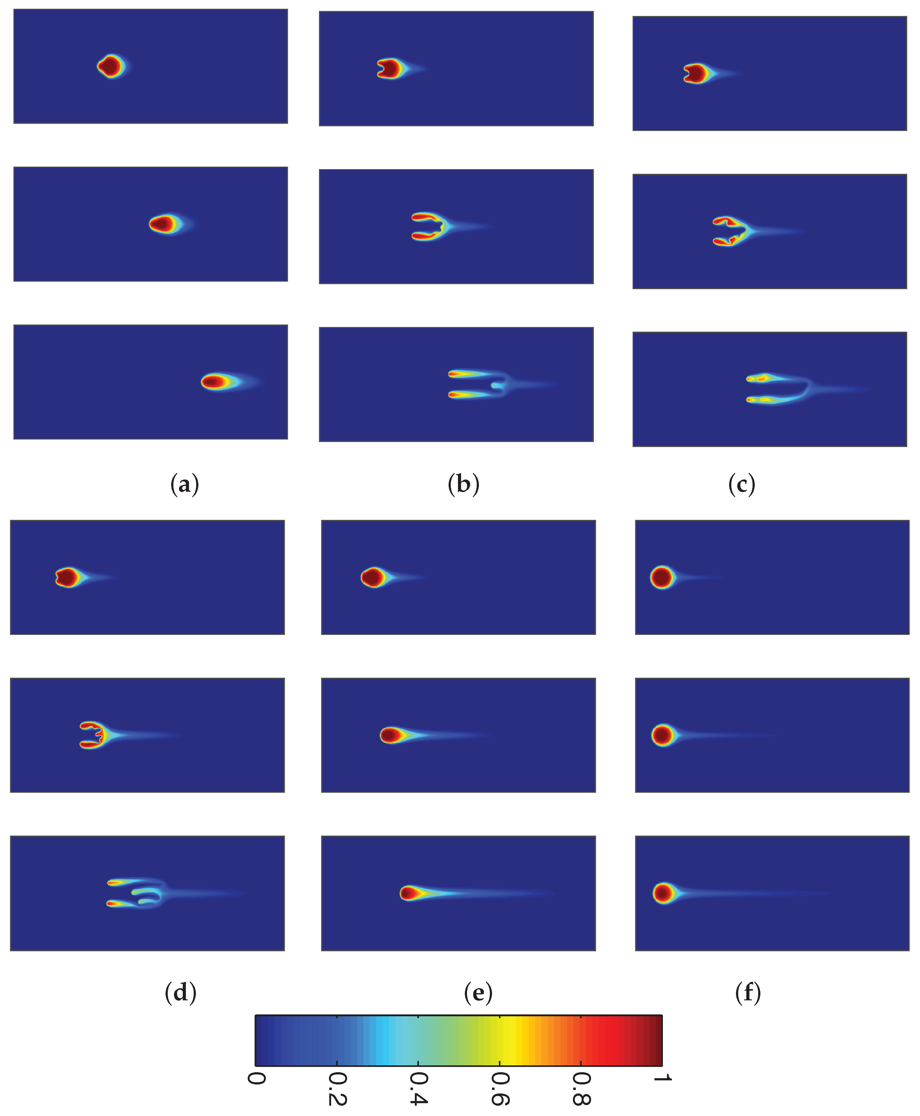
In order to validate our COMSOL modeling, we first, qualitatively reproduce the results of [13]. For a fixed value of Pe $=1000$, the spatio-temporal evolution of the circular blob for six different Rs are shown in Figure 2, which depict the re-entrance into the comet-shaped deformation region from the VF region, while increasing R and keeping Pe fixed. In other words, not all unfavorable viscosity contrasts, but only a finite window of R features VF.

For a given Pe, we define the upper limit of the VF-R window as the critical log-mobility ratio, $R_c^u\left(\mathrm{Pe}\right)$, such that for all $R\ge R_c^u$(Pe) and the given Pe, only comet-shaped deformation is observed [13]. In particular, $R_c^u(\mathrm{Pe}=1000)\approx 2$. In this paper, we primarily explore the dynamics of a more viscous blob for $R\ge R_c^u(\mathrm{Pe}=1000)$, unless otherwise stated.

Figure 2 clearly depicts how increasing viscosity contrast favors and then inhibits VF. Here, we discuss the effect of R for a fixed value of Pe = 1000. For $R=0.5$, convection is weaker than that required for the invading fluid to penetrate into the blob. As a result, the blob deforms into a lump and ultimately into a comet with a small tail. For $0.5<R<2$, the invading fluid penetrates into the blob, resulting in fingering instability at the rear interface and a tail formation at the frontal part of the blob. As we further increase R beyond a critical value ($R_c^u$), the relative velocity of the two fluids increases significantly and the invading fluid prefentially flows around the blob, owing to its curvature [13], and prevents VF. However, the tail formation persists and a long tail is observed at the frontal interface. This preferential flow is clearly visible in Figure 2 at $t=40$ s. The Figure 2e,f depict how the dynamics of the blob change in the comet shape region while increasing the dynamic viscosity of the blob beyond the critical log-mobility ratio. For $R=2$, a tendency to feature VF is observed in the form of a lump (at $t=40$ s), which ultimately changes into a comet with a wide, long tail (Figure 2e). For $R=7$, the mobility of the blob reduces significantly, such that it remains at the same place over the time scale of significant downstream migration of the blob with $R=2$. However, the miscibility and a large relative velocity of the two fluids generate a long narrow tail. As a result, the dynamics of the blob can be described as a stagnant head comet with a downstream developing tail.

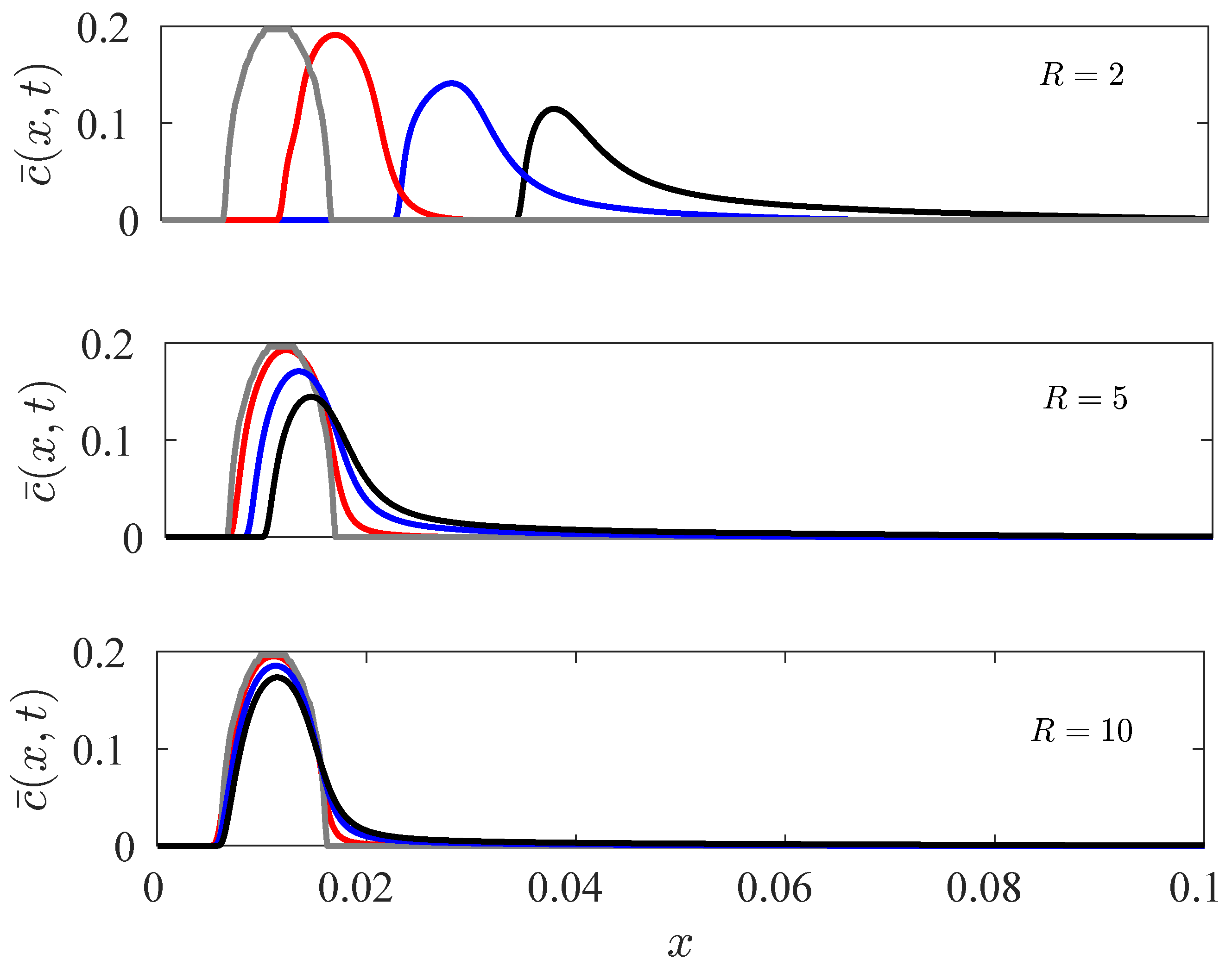
Next, we show that the qualitative features of comet shape blob can be captured from the transversely-averaged concentration,

$$\overline{c}(x,t)=\frac{1}{L_y}{\int }_0^{L_y}c(x,y,t)\mathrm{d}y.$$

(12)

The transversely-averaged concentration of the blob with different orders of viscosity ratio $(\sim \mathcal{O}(1),\mathcal{O}({10}^2)$ and $\mathcal{O}({10}^5))$ are shown in Figure 3.

The characteristics of the blob discussed above can also be described through $\overline{c}(x,t)$. Moreover, the transversely-averaged concentration clearly shows that the width of the tail decreases as the viscosity of the blob increases. A comparison of the position of the maxima at different times for each R in Figure 3 gives a lucid information about the relative mobility of the blobs. The gray line in Figure 3 represents the transversely averaged concentration at $t=0$ seconds for each R. It ensures that the initial position of the blob for each R simulation is the same and works as a reference with respect to which the relative position of the blobs at different times can be compared. It is to be noted that the flat top of the gray line is due to the approximation of a circular arc (of the blob) by rectangular mesh points. Through a grid independence test, we have ensured that the qualitative as well as quantitative dynamics remain unaltered due to this flat top of the gray line. As time progresses, diffusion smoothens the concentration gradient to make the curve smooth as is observed at later times. The increasing viscosity alters the relative velocity of the fluids.

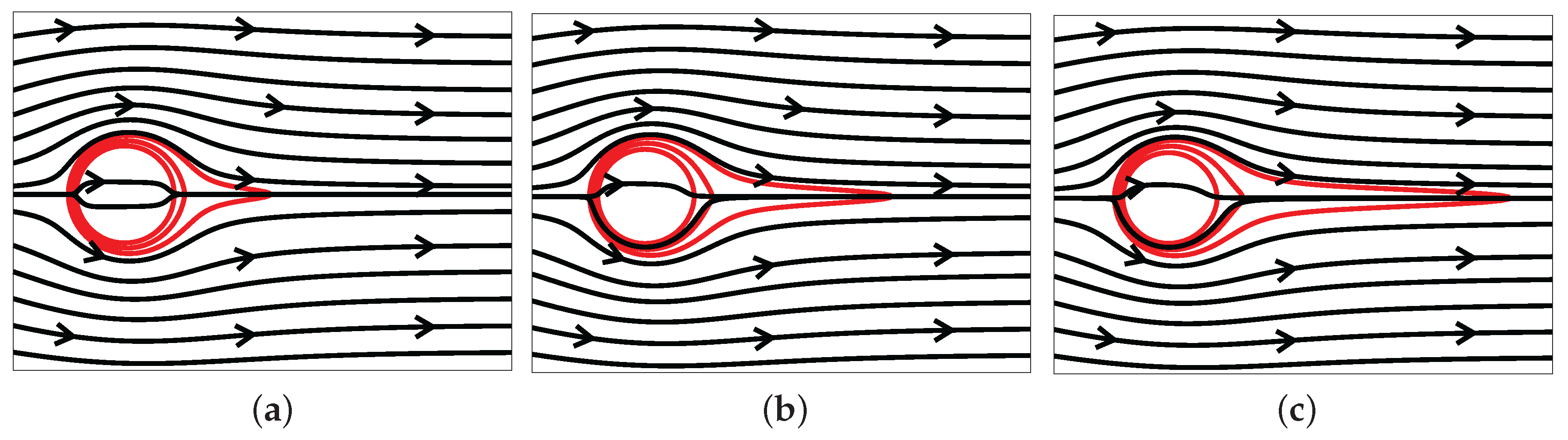
Streamlines are plotted (Figure 4) to have an insight into the instantaneous velocity of fluid. The streamlines near the head of the highly viscous blob appear to be intersecting at a point, but they are actually very close. This is due to the high viscosity contrast, which results in a sudden decrease in the velocity of the fluid near the head. The ambient fluid cannot invade the blob and prefers to flow around it. This is depicted in terms of the sharp bend of the streamlines around the blob. The concentration contours (Figure 4) help to clearly visualize this bend and the breaking in the left–right symmetry due to miscibility of the blob. Streamlines present within the blob (concentration contours) represent the movement of the blob, albeit very small. Thus, there exists no stagnation point, but a point of least velocity near the head of blob. The streamlines of very large viscosity contrast miscible flows exhibit following differences from the streamlines around an erodible body or a solid obstacle in Hele–Shaw cell [25]. First, we discuss the differences between solid obstacle with circular cross section in a Hele–Shaw cell and very large viscosity contrast miscible blob in homogeneous porous media, since the mathematical formulations of the fluid flows in the two cases are analogous. In the former case, the streamlines are symmetric about both the longitudinal and transverse diameters of the circle. On the other hand, for the latter case, the left–right symmetry of the streamlines is broken due to the miscibility of the blob. Next, consider the comparisons between the cases of an erodible body in low-Reynolds number flow [26] and very large viscosity contrasts miscible blob. In both the cases, the left–right symmetry of the streamlines are absent. However, unlike the former, downstream flow separation and upstream stagnation point are not observed in the latter case. This is attributed to the, albeit very small, non-zero fluid velocity within the miscible blob, but no fluid flow inside the erodible body. The upstream deformation of the erodible body or the miscible blob have the similarity that, in both the cases, it takes a streamlined topology. On the other hand, a long tail for the blob, but a flat interface [26] for the erodible body in the downstream direction, marks a dissimilarity between the two.

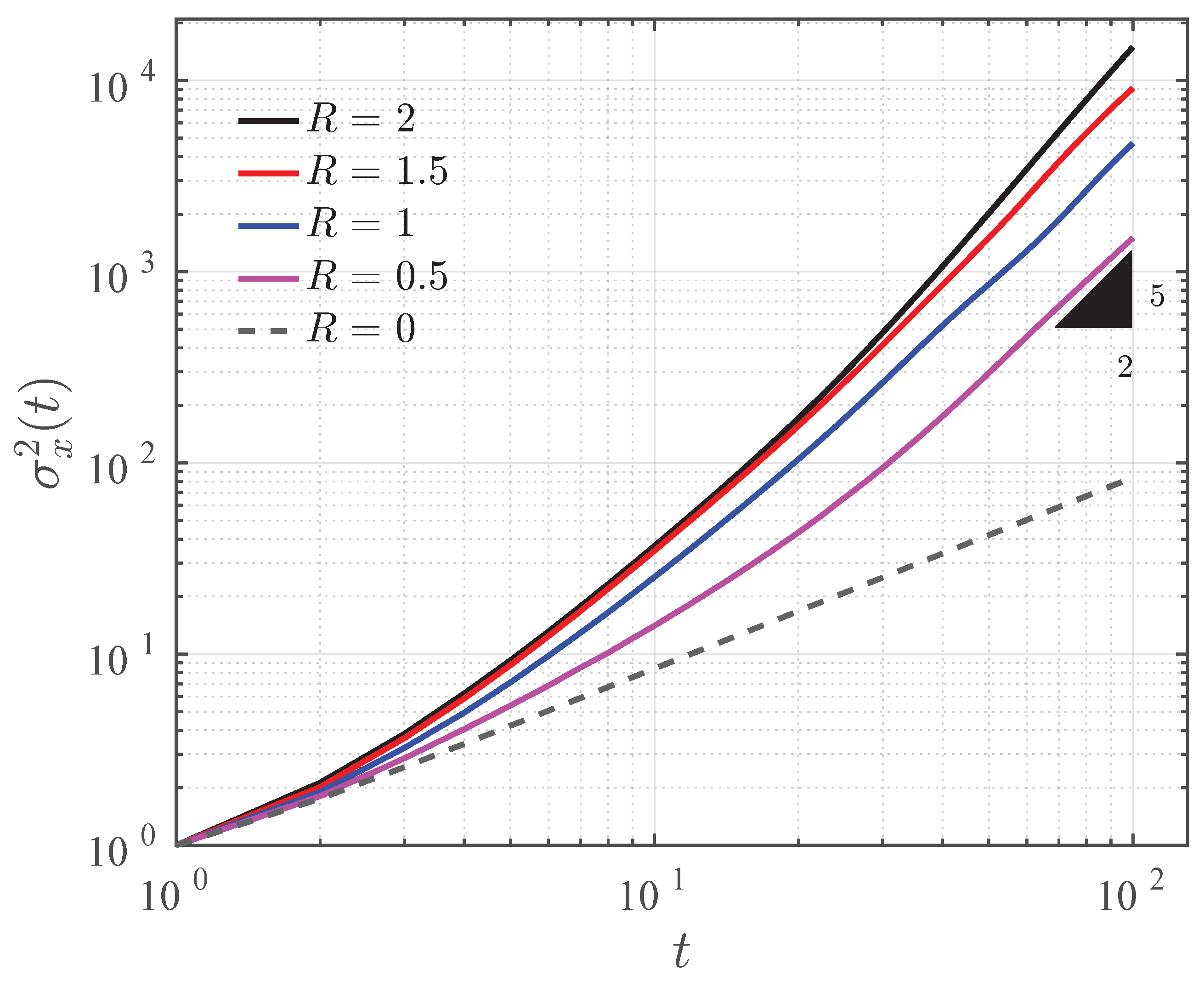
The stream-wise spreading of the blob is quantified in terms of the variance, ${\sigma }_x^2\left(t\right)$, [13,27] of the transversely-averaged concentration, $\overline{c}(x,t)$, defined as

$${\sigma }_x^2\left(t\right)=\frac{{\int }_0^{L_x}{\left[x-m\left(t\right)\right]}^2\overline{c}(x,t)\mathrm{d}x}{{\int }_0^{L_x}\overline{c}(x,t)\mathrm{d}x}.$$

(13)

Here,

$$m\left(t\right)=\frac{{\int }_0^{L_x}x\overline{c}(x,t)\mathrm{d}x}{{\int }_0^{L_x}\overline{c}(x,t)\mathrm{d}x}$$

(14)

is the mean of $\overline{c}(x,t)$. In order to refrain the numerical error to contaminate variance, ${\sigma }_x^2\left(t\right)$, we rescale the variance given by Equation (13) as

$$\frac{{\sigma }_x^2\left(t\right)-{\sigma }_x^2(t=0)}{{\sigma }_x^2(t=1)-{\sigma }_x^2(t=0)}\to {\sigma }_x^2\left(t\right).$$

(15)

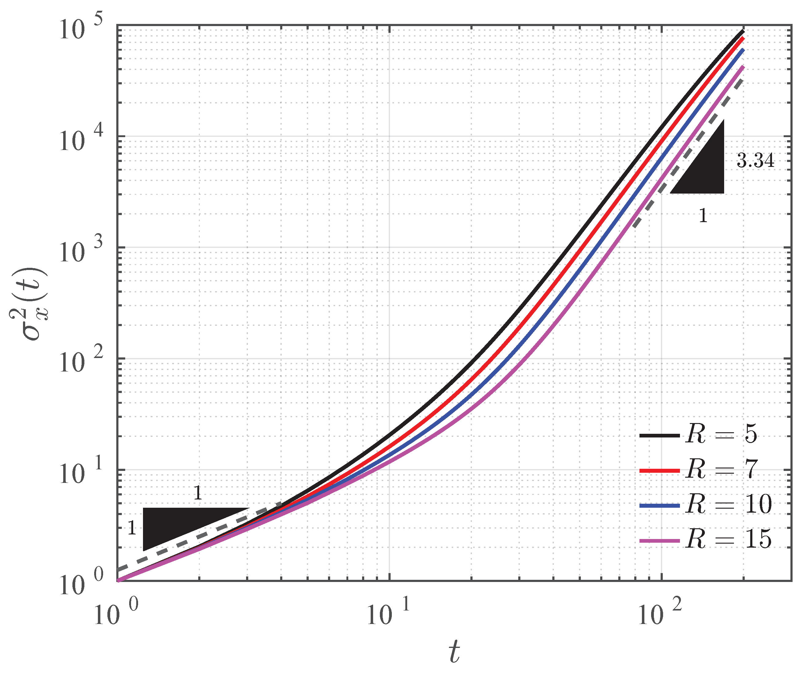
Figure 5 and Figure 6 show the log-log plot of the temporal evolution of the rescaled variance, which is denoted by the same notation as of the variance defined in Equation (13). For $0<R<2.5$ and Pe $=1000$, Pramanik et al. showed that ${\sigma }_x^2\sim t$ at early times, while at later times, ${\sigma }_x^2\sim t^{5/2}$ [13]. We are successful at reproducing these power-law results using our COMSOL modeling (Figure 5). This further confirms the validity of our COMSOL model. We are interested to know the power-law behavior of ${\sigma }_x^2$ for very large viscosity contrasts. For all values of $R>0$, early time behavior of ${\sigma }_x^2$ is identical to that of $R=0$. The instance of departure of ${\sigma }_x^2$ from the linear time variation depends on the value of R. After that, there is a R-dependent intermediate time interval for the transition from the linear time variation to another power-law variation of ${\sigma }_x^2$. For viscosity ratio in the range $\mathcal{O}({10}^2)$–$\mathcal{O}({10}^6)$, ${\sigma }_x^2\sim t^{3.34}$ (see Figure 6).

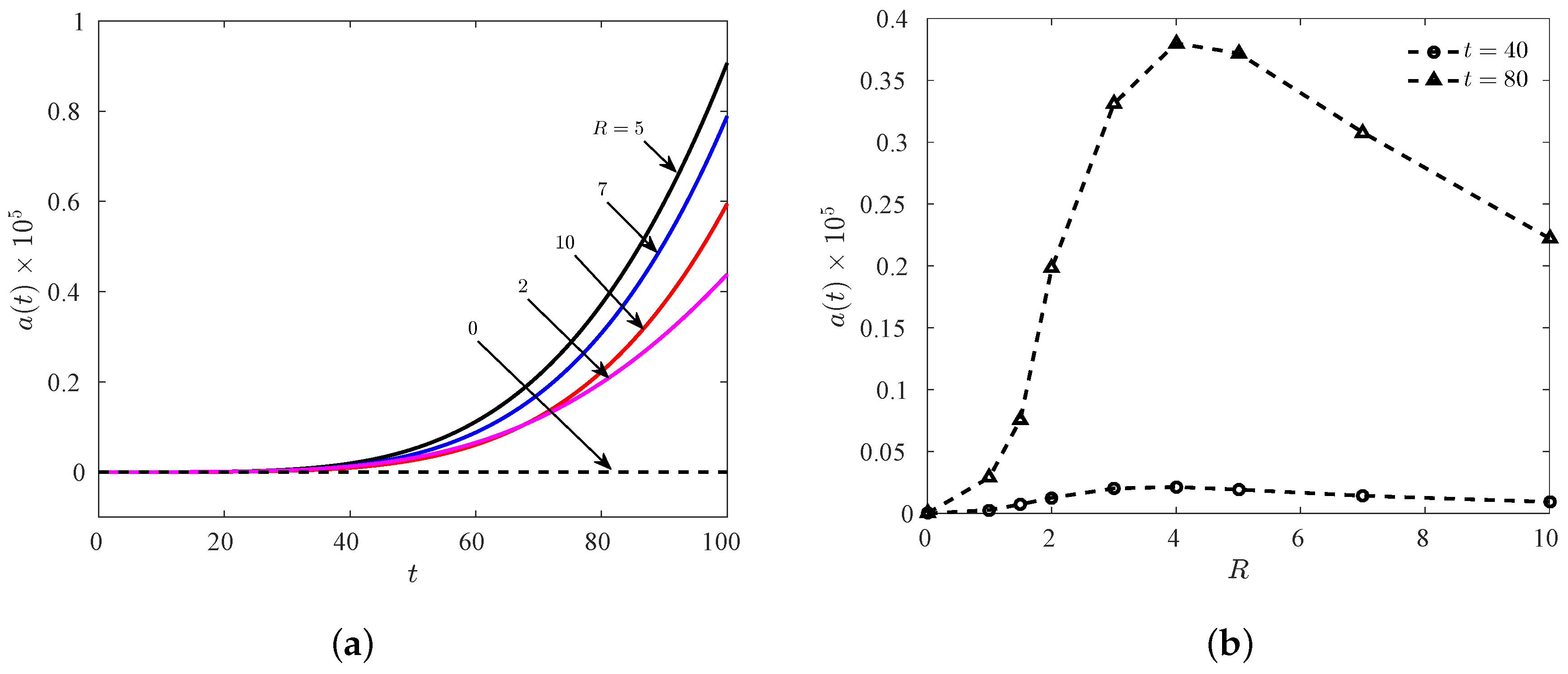
Furthermore, in order to quantify the left–right asymmetry of the blob, we measure a statistical quantity, the skewness [28] of transversely-averaged concentration $\overline{c}(x,t)$,

$$a\left(t\right)=\frac{{\int }_0^{L_x}{\left[x-m\left(t\right)\right]}^3\overline{c}(x,t)\mathrm{d}x}{{\int }_0^{L_x}\overline{c}(x,t)\mathrm{d}x}.$$

(16)

The effect of R on the asymmetry is examined by plotting skewness as a function of time in Figure 7a, which shows that $a\left(t\right)$ increases with t for all R. This represents the asymmetry increases as time progresses in accordance with the increasing length of the downstream tail of the comet. Furthermore, at a fixed later time, skewness varies non-monotonically with R as shown in Figure 7b. This is a consequence of the re-entrance into the comet formation region for very high viscosity contrast. In the $R\ge R_c^u$ comet formation region, a long tail is formed at the front interface, resulting in more asymmetry than that for $R<R_c^l$. 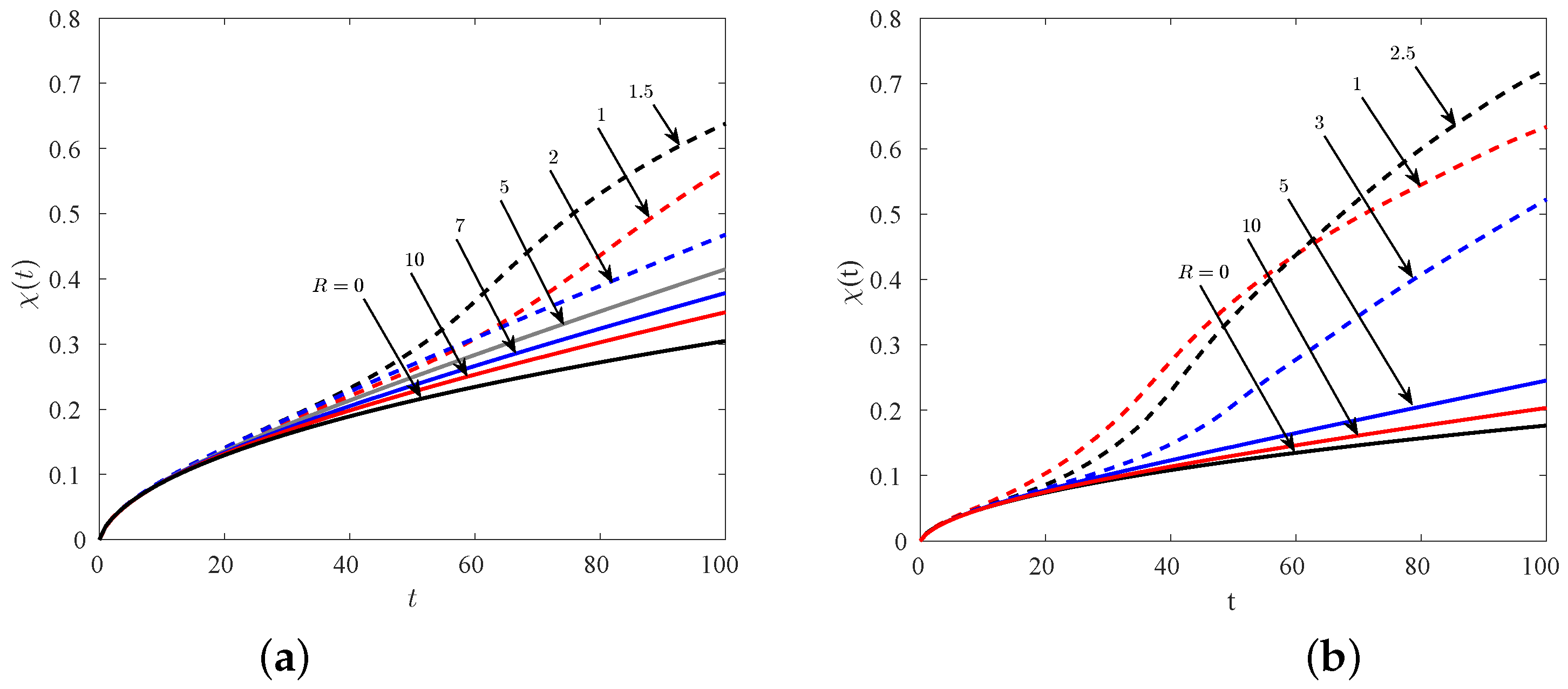However, for very high viscosity contrast $\sim \mathcal{O}({10}^3)$ and even higher, the width of tail decreases, which causes a reduction in the asymmetry. Nevertheless, the asymmetry never vanishes, since the tail formation persists with viscosity contrast of all orders feasible with the current numerical computations. We also calculated the degree of mixing [29,30],

$$\chi \left(t\right)=1-\frac{{\sigma }^2\left(t\right)}{{\sigma }_{\max }^2},$$

(17)

where ${\sigma }^2(t)\equiv \langle c^2\rangle -{\langle c\rangle }^2$ is the global variance of concentration, and ${\sigma }_{\max }^2$ is its maximum value. This is a measure of mixing of the viscous blob with the ambient fluid.

In the present study, mixing is attributed to diffusive spreading, VF and tail formation. Figure 8a shows the temporal evolution of $\chi \left(t\right)$ for a wide range of R for $\mathrm{Pe}=1000$. This figure depicts that, at early times ($t\le 15$), $\chi \left(t\right)$ is almost identical for all R, as, initially, diffusion dominates and mixing is due to diffusive spreading. At later times, the degree of mixing of the blob with the ambient fluid has a non-trivial dependence on R. For $R_c^l<R<R_c^u$, the rear interface of the blob undergoes VF, in addition to a tail formation at the frontal interface. Consequently, the area of contact between the two fluids increases [29], which eventually increases mixing. However, as R is increased beyond $R_c^u$, the front interface deforms into a tail and no VF is observed. In addition, as is evident from Figure 2 and Figure 3, the width of the tail and hence the area of contact between the two fluids decreases, as we keep on increasing the viscosity contrast between the fluids. Ultimately, for $R>R_c^u$, the degree of mixing is found to approach the viscosity-matched case, for which mixing is only due to diffusive spreading, hence $\chi \left(t\right)$ is the minimum for this case $(R=0)$. Figure 8b mimics the same qualitative features for $\mathrm{Pe}=3000$ at different R. However, a comparison of the corresponding curves for $R=5,10$ in both the figures shows a smaller mixing for higher Pe. This is because, increasing Pe decreases the diffusion between the two fluids, which decreases the width of the tail and hence the mixing.

4. Discussion and Conclusions

Although numerical simulations of miscible VF remained in the forefront of active research over the decades, these studies remained restricted to either moderate diffusion or viscosity contrast. To the best of our knowledge, recent studies succeeded in capturing the VF dynamics for $R\approx 7$ [20]. For either case of large R or Pe, sharp velocity gradients at the finger tips cause problems with convergence of the numerical results. Here, we use an FEM-based COMSOL simulator and discuss some interesting and previously unexplored dynamics of miscible blobs in homogeneous porous media with very large viscosity contrasts.

Time discretization of the numerical scheme plays a very important role in deciding its fate (convergence or divergence). The explicit time discretization schemes are conditionally stable, allowing convergent results only for a limited value of the time or space discretization. Similarly, the semi-implicit time discretization schemes are found to show convergence only for some parameters. The Fourier pseudo-spectral method used by various researchers [9,13] to capture non-linear VF, is an example of the semi-implicit time discretization. This pseudo-spectral method converges only for $R\le 3$. Meiburg and Chen [19] adapted a compact finite difference and the ADI method to simulate miscible VF in both homogeneous and heterogeneous porous media. They captured a new VF mechanism called side branching. However, they also could not go higher than $R=5$. The reason for this non-convergence was found to be the explicit nature of the scheme [20]. In addition, when the viscosity contrast between the miscible fluids is high, there exists a sharp velocity gradient and slow concentration variation across the interface, making the problem stiff. Hence, for exploring the flow of the fluids with viscosity $\mathcal{O}({10}^4)$, an implicit time-discretization with a stiff system solver may be helpful. In COMSOL, we used backward differentiation formulas of first and second orders, with the implicit time solvers known for their A-stability [31]. Allowing the time stepping to be adaptive, and uniform spatial step size sufficient to capture the finest fingers and avoid numerical diffusion, helped us to obtain convergent results for very large viscosity contrast between the fluids ($R\approx 15$). We showed that, for a high viscosity contrast, there exist remarkable similarities and dissimilarities between the flow around an erodible body and the flow of a less viscous fluid around a highly viscous miscible blob. Although there exists no stagnation point in the case of the latter, the huge viscosity contrast results in a considerable decrease in velocity near the interface. This decrease in velocity forms a reason for the non-existence of VF even with an unfavorable viscosity contrast for high viscosity blobs. Owing to miscibility, only a tail is observed at the frontal interface, motivating us to compare with the flow around erodible bodies. We also capture and discuss the breaking in the left–right symmetry of the streamlines around the blob, a distinction between the flow around highly viscous blob and the Hele–Shaw flow around a solid body, although both of the problems are mathematically analogous. In the presence of an unfavorable but very high viscosity contrast $\sim \mathcal{O}({10}^4)$ or $R=10$, mixing and spreading of the blob is quantitatively similar to those of a blob in the ambient fluid of same viscosity, that is, when $R=0$. Initial time evolution of the variance of transversely averaged concentration (Figure 6) and skewness (Figure 7a) justify this. The spreading for a high viscous blob follows the power law ${\sigma }_x^2\left(t\right)\sim t^{3.34}$, and the degree of mixing varies non-monotonically with the log-mobility ratio R. This can be attributed to the effect of curvature, which results in re-entrance into the comet formation regime, decreasing the area of contact and hence the degree of mixing with an increase in R. $\chi \left(t\right)$ for the highly viscous blob approaches that for the viscosity matched case, independent of the Pe. In addition, it is found that there is no tendency of VF formation in the case of highly viscous blobs, as there is no lump formation initially, which is evident for blobs with log-mobility ratio $\sim R_c^u$. Thus, we conclude that curvature plays a very important role in the displacement processes involving viscosity contrast, and the dynamics of a highly viscous blob can be explored further to compare to that of an erodible body and to understand heavy oil extractions.

Hence, the COMSOL simulations software used wisely can be applicable to understand fingering instability, mixing, and other qualitative as well as quantitative behaviors in the presence of additional disturbances to the system, such as dispersion anisotropy, permeability heterogeneity, heterogeneous porosity, velocity-dependent dispersion, adsorption, and many more, which may result in numerical instabilities to the spectral solution of the stream function formulation. An equation-based model using the COMSOL Multiphysics with more degrees of freedom in terms of the boundary conditions, domain discretization, and incorporating additional body (surface) forces into the transport equations will be considered in future research.