Theoretical Analysis of Cuttings Accumulation at Curvature Transition Zones in Double Build-Up Wells

Abstract

Extended-reach and highly deviated wells often adopt a double build-up trajectory. This profile contains two curvature transition zones: the build-to-tangent transition and the tangent-to-build transition. The annular flow undergoes severe restructuring in these zones. They are potential bottlenecks for cuttings transport. This work uses a 215.9 mm wellbore with 127.0 mm drill pipe as the reference case. Analytical expressions for the cuttings accumulation ratio in both transition zones are developed based on the three-layer transport model. For power-law drilling fluids, a generalized Reynolds number is introduced to reformulate the Dean number. A dynamic disturbance coefficient is constructed from the along-hole Dean number gradient. This coefficient captures the contrasting behavior of secondary flow. In one transition zone, the secondary-flow decays. In the other, it suddenly emerges. The results show that when the two curvature radii are equal, the accumulation ratio in the tangent-to-build transition is roughly 1.15 times that in the build-to-tangent transition. Reducing the curvature radius from 250 m to 100 m increases the accumulation ratio by about 2.5 times. The ratio rises with the inclination angle. The disturbance coefficient increases monotonically with the build rate. After accounting for drill pipe eccentricity, the recommended minimum curvature radii are 160 m for the first build section and 220 m for the second. These findings offer a theoretical basis for trajectory design in sections with abrupt curvature changes.

1. Introduction

Hole cleaning remains a persistent challenge in extended-reach and highly deviated wells. In these well geometries, cuttings travel from the bottom-hole annulus to the surface. They pass through horizontal, build, tangent, and vertical sections. As inclination builds and lateral reach increases, cuttings tend to settle on the low side of the wellbore. They form beds that raise both torque and drag. This degrades drilling performance. In severe cases, it can lead to stuck pipe. The annular clearance in 8½ in holes is relatively narrow. This makes localized accumulation and bridging more likely than in larger or more conventional wellbore sizes [1].

The literature on cuttings transport modeling is extensive. Early experiments identified four distinct flow regimes in inclined annuli. These are uniform suspension, non-uniform suspension, moving bed, and stationary bed. Each regime has its own critical velocity threshold [2]. The three-layer model divides the annulus into a suspended layer, a dispersed layer, and a stationary bed. This offers a more realistic description than the simpler two-layer approach [3]. Guo et al. [4] developed a steady-state three-layer model for extended-reach wells. They found that annular velocity is the single most influential factor. The dominant transport mechanisms vary significantly across inclination ranges. Zhao et al. [5] later incorporated transient effects through a coupled unsteady model.

Critical transport velocity provides a practical metric for assessing hole cleaning. Larsen [6,7] conducted extensive flow-loop tests and developed a dedicated model for highly deviated wells, capable of predicting both the critical velocity and the resulting cuttings concentration profile. Yang et al. [8] observed that the inclination range of 40° to 50° is particularly prone to bed formation and that increasing rotary speed substantially improves cleaning.

Drill pipe eccentricity and rotation have drawn increasing attention in recent years. In high-angle sections, the pipe lies against the low side of the borehole under gravity. This creates an eccentric annulus with a marked velocity asymmetry. Flow is high in the wide upper gap and low in the narrow lower gap. Eddies tend to form in the lower gap [9]. Sun et al. [10] showed through Eulerian two-phase simulations that the helical flow induced by pipe rotation can disturb the bed and re-entrain particles. An eccentricity of 0.5 is commonly assumed for the 215.9 mm hole and 127.0 mm pipe combination [11]. In curved build sections, the bending of the wellbore further forces the pipe against the wall. This alters the flow distribution between wide and narrow gaps [12]. Field observations confirm that cuttings beds are common in both horizontal and build sections. They have measurable effects on drill string mechanics [13].

Despite this body of work, most studies have focused on constant-inclination sections and have not systematically examined the two curvature transition zones in a double build-up profile. This study addresses that gap. Starting from the three-layer framework, we derive analytical expressions for the accumulation ratio at both transitions. A curvature correction term is introduced to account for the effect of wellbore curvature on the critical velocity, while pipe eccentricity is treated separately. For power-law fluids, we modify the Dean number using a generalized Reynolds number and construct a dynamic disturbance coefficient from the along-hole gradient of the Dean number. This coefficient distinguishes between two physically distinct scenarios: one where secondary flow gradually decays and one where it abruptly emerges. The objectives are to clarify the fundamental difference between the two transition zones, quantify their sensitivity to curvature radius, and provide practical design charts and recommended values for trajectory optimization.

2. Theoretical Model

This section develops an analytical model for cuttings accumulation in the two curvature transition zones. We begin with the governing equations and assumptions of the three-layer transport model then derive the critical velocity through single-particle force balance. A curvature correction is applied to account for the abrupt flow-field changes in the transition zones. Finally, an accumulation ratio is defined based on the balance between deposition and resuspension.

2.1. Basic Framework of the Three-Layer Model

We adopt the classical three-layer description of cuttings transport [14]. The suspended layer occupies the upper part of the annulus, where cuttings are fully entrained at a low solids fraction. The dispersed layer lies in the middle, where particles move by saltation and rolling along the low side. The stationary bed sits at the bottom, consisting of deposited cuttings that are no longer in motion. Mass and momentum are exchanged across the interfaces between these layers.

The following assumptions are made:

(1)

Flow is one-dimensional and steady along the wellbore.

(2)

Properties are uniform within each layer.

(3)

Cuttings are uniform spheres of equal diameter.

(4)

Interlayer mass exchange is neglected, but momentum transfer is retained.

(5)

The drilling fluid obeys the power-law rheological model.

(6)

Pipe eccentricity is fixed at e = 0.5. A correction function is applied to the accumulation ratio to account for eccentricity.

Admittedly, the one-dimensional steady-state assumption does not resolve the full three-dimensional structure of secondary flows in curved sections. Dean vortices do arise from centrifugal effects and redistribute momentum across the annulus. The present analysis, however, is not concerned with the detailed distribution of these vortices but rather with their net influence on bed accumulation, which we link to the streamwise variation in secondary-flow intensity. This is captured through the generalized Dean number and the resulting disturbance coefficient. It should be emphasized that the present model does not resolve the three-dimensional transient development or decay of Dean vortices at curvature transition zones; rather, it captures only the net effect through the generalized Dean number and the disturbance coefficient.

The quantitative uncertainty associated with this simplification remains to be assessed through future experimental measurements or high-fidelity CFD simulations. For most field applications where curvature changes are gradual, the loss of fidelity is unlikely to compromise the main conclusions. For cases with rapid curvature changes, however, the model predictions should be interpreted with due caution.

2.2. Mass Conservation Equations

Under steady flow, the mass conservation equations for the three layers are as follows:

The suspended layer

$${\displaystyle \frac{d}{ds}}(A_s{\rho }_l{C}_{l,s}{v}_{l,s}+A_s{\rho }_s{C}_{s,s}{v}_{s,s})=0$$

(1)

The dispersed layer

$${\displaystyle \frac{d}{ds}}(A_d{\rho }_l{C}_{l,d}{v}_{l,d}+A_d{\rho }_s{C}_{s,d}{v}_{s,d})=0$$

(2)

The stationary bed layer

$${\displaystyle \frac{d}{ds}}(A_b{\rho }_s{C}_{s,b}{v}_{s,b})=0$$

(3)

Here, s is the coordinate along the wellbore, A_s, A_d and A_b are the cross-sectional areas of the three layers, and C denotes volume fraction. Subscripts l and s stand for liquid and solid, and v is velocity. The total annular area satisfies A = A_s + A_d + A_b.

2.3. Momentum Conservation Equations and Accumulation Ratio

The momentum equations for the three layers are as follows:

The suspended layer

$${\displaystyle \frac{d}{ds}}(A_s{\rho }_l{C}_{l,s}{v}_{l,s}^2+A_s{\rho }_s{C}_{s,s}{v}_{s,s}^2)=-A_s{\displaystyle \frac{dp}{ds}}-A_s{\rho }_{m}g\cos \theta -{\tau }_{s-w}{S}_s-{\tau }_{s-d}{S}_{sd}$$

(4)

The dispersed layer

$${\displaystyle \frac{d}{ds}}(A_d{\rho }_l{C}_{l,d}{v}_{l,d}^2+A_d{\rho }_s{C}_{s,d}{v}_{s,d}^2)=-A_d{\displaystyle \frac{dp}{ds}}-A_d{\rho }_{m}g\cos \theta -{\tau }_{d-w}{S}_d+{\tau }_{s-d}{S}_{sd}-{\tau }_{d-b}{S}_{db}$$

(5)

The stationary bed layer

$${\tau }_{d-b}{S}_{db}=A_b{\rho }_s{C}_{s,b}g\cos \theta +F_{friction}$$

(6)

where p is pressure, θ is the inclination angle, ρ_m = C_lρ_l + C_sρ_s is the mixture density, τ represents shear stress at various interfaces, S is the wetted perimeter, and F_friction is the bed–wall friction force.

The forces acting on a single cuttings particle include gravity, buoyancy, drag, and lift:

$$F_g={\displaystyle \frac{\pi d_s^3}{6}}{\rho }_{s}g$$

(7)

$$F_b={\displaystyle \frac{1}{6}}\pi d_s^3{\rho }_{l}g$$

(8)

$$F_d={\displaystyle \frac{1}{2}}{C}_D{\rho }_l{A}_p{(v_l-v_s)}^2$$

(9)

$$F_l={\displaystyle \frac{1}{2}}{C}_L{\rho }_l{A}_p{(v_l-v_s)}^2$$

(10)

where d_s is the cuttings particle diameter, A_p = πd_s²/4 is the particle projected area, C_D is the drag coefficient, C_L is the lift coefficient, and v_l and v_s are the phase velocities. Incipient motion occurs when the combined drag and lift exceed the gravitational component and friction.

The Larsen model gives the critical velocity as

$$v_{cr}=v_{cr}(\theta ,{\rho }_l,{\rho }_s,d_s,\mu ,e)$$

(11)

In curved sections, Dean vortices alter the velocity profile and thus affect the critical velocity. Following Larsen’s approach for curved conduits, we introduce a curvature correction:

$$v_{cr,trans}=v_{cr,stable}(\theta )\cdot \left[1+\lambda \cdot {\displaystyle \frac{d\theta }{ds}}\right]$$

(12)

where v_cr,stable(θ) is the value under straight-inclined conditions, dθ/ds = 1/R is the build rate, R is the radius of curvature, and λ is a curvature influence coefficient. For Transition Zone I, this correction captures the residual effect of upstream curvature; for Transition Zone II, it reflects the pre-disturbance from the downstream build section.

The bed thickness in the transition zone is governed by the balance between deposition and resuspension:

$${\displaystyle \frac{d{h}_b}{ds}}={\displaystyle \frac{{\dot{m}}_{dep}-{\dot{m}}_{ent}}{{\rho }_b(1-\varphi )}}$$

(13)

where ${\dot{m}}_{dep}$ and ${\dot{m}}_{ent}$ are the deposition and resuspension rates, ρ_b is the bed bulk density, and ϕ is the bed porosity.

The deposition rate depends on the difference between actual velocity and the critical velocity. Substituting the corrected critical velocity gives

$${\dot{m}}_{dep,trans}\propto C_s\cdot \max \left[v_{cr,stable}(\theta )\left(1+{\displaystyle \frac{\lambda }{R}}\right)-v_l,0\right]$$

(14)

We define the accumulation ratio η and introduce the eccentricity correction f(e):

$$\eta ={\displaystyle \frac{h_{b,trans}-h_{b,stable}}{h_{b,stable}}}={\displaystyle \frac{\lambda }{R}}\cdot {\displaystyle \frac{v_{cr,stable}}{v_l-v_{cr,stable}}}\cdot f(e)$$

(15)

where h_b,trans is the bed height in the transition zone, h_b,stable is the steady-state value in the upstream tangent section, and the value f(e) = 1.15 at the specified drill pipe eccentricity e = 0.5 [15].

2.4. Unified Formulation and Dynamic Difference Between the Two Transition Zones

Applying Equation (12) to the two transition zones gives the following.

Transition Zone I (build to tangent) is

$$v_{cr,trans1}=v_{cr,stable}(\theta )\cdot \left[1+{\displaystyle \frac{\lambda }{R_1}}\right]$$

(16)

Transition Zone II (tangent to build) is

$$v_{cr,trans2}=v_{cr,stable}(\theta )\cdot \left[1+{\displaystyle \frac{\lambda }{R_2}}\right]$$

(17)

The accumulation ratio can be written in a unified form:

$$\eta ={\displaystyle \frac{\lambda }{R}}\cdot {\displaystyle \frac{v_{cr,stable}}{v_l-v_{cr,stable}}}\cdot f(e)$$

(18)

This expression applies to either transition zone. The only differences between the two zones are the specific value of the curvature radius and the direction of the flow-field change.

However, Equation (18) captures only the static effect of curvature radius. It does not account for the dynamic disturbance caused by the abrupt change in the flow field. This disturbance depends on whether secondary flow is decaying or being generated.

When fluid flows through a curved conduit, centrifugal force generates secondary flow perpendicular to the main flow direction. Dean [16] first characterized this phenomenon and introduced the Dean number as a dimensionless measure of secondary-flow intensity. In curved wellbore sections, Dean vortices distort the annular velocity profile, creating a pair of counter-rotating eddies that affect cuttings transport.

For the rheological description, we adopt the power-law model rather than the more general Herschel–Bulkley form. This choice is motivated by two considerations. First, under the elevated shear rates that prevail in the annular flow of this study, the yield stress of the drilling fluid contributes little to the overall stress, so the power-law simplification introduces negligible error. Second, the power-law form permits a closed-form expression for the generalized Dean number, which is central to the present framework. The constitutive relation is given by $\tau =K{\left({\displaystyle \frac{d\mu }{dy}}\right)}^n$, where K denotes the consistency index and n is the flow-behavior index. The generalized Reynolds number for power-law fluids is defined as

$$R{e}_{pl}={\displaystyle \frac{\rho v_{ann}^{2-n}{D}_{ann}^n}{K{\left(\frac{4n}{3n+1}\right)}^n{8}^{n-1}}}$$

(19)

Substituting this generalized Reynolds number Re_pl into the standard Dean number formulation yields the modified generalized Dean number for power-law fluids:

$$D{e}_{pl}(s)=R{e}_{pl}\cdot \sqrt{{\displaystyle \frac{D_{ann}}{2R(s)}}}$$

(20)

Here, R(s) is the curvature radius as a function of measured depth s. In tangent sections, R → ∞; in constant-curvature build sections, R is finite and constant. The axial variation of De_pl describes how secondary-flow strength changes along the trajectory.

The disturbance intensity acting on the cuttings bed scales with the absolute value of the axial gradient of De_pl. We define a dynamic disturbance amplification f factor ψ(s) as the ratio of this intensity in Transition Zone II to that in Transition Zone I:

$$\psi (s)={\displaystyle \frac{|dD{e}_{pl}/ds{|}_{II}}{|dD{e}_{pl}/ds{|}_I}}$$

(21)

where the subscripts indicate the paths across the two transition zones. From Equation (20), the gradient can be expanded as

$${\displaystyle \frac{dD{e}_{pl}}{ds}}=R{e}_{pl}\sqrt{{\displaystyle \frac{D_{ann}}{2}}}\cdot {\displaystyle \frac{d}{ds}}\left(R{(s)}^{-1/2}\right)$$

(22)

This gradient has two contributions. One comes from the variation in the generalized Reynolds number. This captures rheology and flow-rate effects. The other comes from the variation in the curvature radius. This describes how rapidly the trajectory changes. A faster curvature change produces a larger Dean number gradient and thus a larger ψ. Higher build rates generate stronger secondary-flow disturbances in Transition Zone II.

For constant-curvature build sections, R is constant and R^−1/2 undergoes a step change at the transition boundary. The ratio of the Dean number gradients then reduces to

$$\psi \approx {\displaystyle \frac{1/R_2}{1/R_1}}={\displaystyle \frac{R_1}{R_2}}$$

(23)

when R₁ = R₂, ψ ≈ 1. Physically, however, the sudden onset of secondary flow in Transition Zone II produces a stronger disturbance than the gradual decay in Transition Zone I. We therefore introduce an enhancement coefficient β > 1 to account for this impulsive effect. The physical origin of β is the incipient-motion lag of bed particles. Stationary particles require a larger force to start moving again.

We acknowledge that the value β = 1.15 falls slightly below the experimental range of 1.2–1.5 reported by Kim and Patel [15] for rectangular ducts. Given the annular geometry of wellbore hydraulics, we adopted the lower-bound value as a provisional engineering assumption in the absence of directly applicable annular-flow data. This choice preserves the impulsive effect of secondary-flow emergence in Transition Zone II, since this qualitative effect requires only β > 1. The quantitative validity of this assumption should be subject to future experimental or numerical validation in annular geometries. This choice is further supported by the findings of Saffar et al. [17], who demonstrated that the streamwise gradient of the Dean number, rather than its absolute value, governs the disturbance intensity. The present modeling approach aligns with that rationale.

The final form of the amplification factor is

$$\psi =\beta \cdot {\displaystyle \frac{R_1}{R_2}}$$

(24)

when R₁ = R₂, ψ ≈ 1.15.

The ratio of the accumulation ratios for the two transition zones is

$${\displaystyle \frac{{\eta }_2}{{\eta }_1}}=\psi \cdot {\displaystyle \frac{R_1}{R_2}}=\beta \cdot {\left({\displaystyle \frac{R_1}{R_2}}\right)}^2$$

(25)

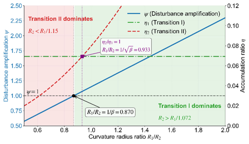
when R₁ = R₂, η₂/η₁ = β ≈ 1.15. When R₂ > 1.072R₁, η₂/η₁ < 1, and Transition Zone I becomes the more critical condition. When R₂ > 1.15R₁, ψ < 1, meaning that the secondary-flow disturbance in Transition Zone II has dropped below that in Transition Zone I.

The complete expressions for the accumulation ratios are

$${\eta }_1={\displaystyle \frac{\lambda }{R_1}}\cdot {\displaystyle \frac{v_{cr,stable}}{v_l-v_{cr,stable}}}\cdot f(e)$$

(26)

$${\eta }_2=\psi \cdot {\displaystyle \frac{\lambda }{R_2}}\cdot {\displaystyle \frac{v_{cr,stable}}{v_l-v_{cr,stable}}}\cdot f(e)$$

(27)

3. Parametric Analysis and Mechanism Investigation

This section presents a systematic parametric analysis using the analytical model derived above. It quantifies how key governing factors affect cuttings accumulation in the two transition zones, ranks these parameters by their relative influence, and yields trajectory optimization charts that can be directly adopted in field design.

3.1. Basic Parameters and Calibration of λ

The drilling fluid is modeled as a power-law fluid.

Table 1. Basic calculation parameters.

Parameter	Symbol	Value
Wellbore diameter (mm)	Dh	215.9
Drill pipe outer diameter (mm)	Dp	127.0
Annular equivalent diameter (mm)	Dann	Dh − Dp = 88.9
Annular cross-sectional area (m2)	A	0.024
Drilling fluid density (kg/m3)	ρl	1350
Cuttings density (kg/m3)	ρs	2650
Cuttings particle diameter (mm)	ds	2.0
Circulation flow rate (L/s)	Q	33
Annular flow velocity (m/s)	vl	1.38
Power-law consistency index (Pa·sn)	K	0.35
Power-law flow-behavior index	n	0.65
Drill pipe eccentricity	e	0.5
Eccentricity correction factor	f(e)	1.15

lists the input parameters.

The parameters in Table 1 are derived from field measurements and drilling design specifications for the Jidong Oilfield.

3.1.1. Threshold for the Accumulation Ratio η

The accumulation ratio η is defined as the fractional increase in bed height relative to the steady-state value in the upstream tangent section. Values of 0.10 and 0.15 correspond to 10% and 15% increases, respectively.

Zhu et al. [18] proposed using the fraction of wellbore length where the bed height exceeds 10% of the well diameter as a cleaning metric; below this threshold, the well is considered adequately clean. For the 8½ in hole considered here, 10% of the diameter corresponds to about 21.6 mm. Jing et al. [19] reported prediction errors below 10% for their bed-height model over a wide range of conditions, supporting the use of these thresholds.

We adopt 0.10 as the baseline threshold for acceptable cleaning and 0.15 as the onset of significant accumulation. These values are reference values and can be adjusted for specific field conditions. If enhanced cleaning measures are used, such as a higher flow rate, increased rotary speed, or bed-breaking tools, the allowable η may be relaxed to 0.12–0.15. In more challenging conditions, such as a very long tangent section or unstable formations, the threshold should be tightened to 0.08–0.10.

The thresholds 0.10 and 0.15 are adopted here as reference points rather than absolute limits. They are appropriate for the water-based mud and the range of conditions assumed in the parametric study. When oil-based muds are used, which typically have better carrying capacity, the allowable η might be raised to 0.12–0.15. In contrast, troublesome intervals such as unstable formations or very long tangent sections may warrant a tighter criterion of 0.08–0.10. These thresholds should be adjusted according to local experience and specific well constraints.

3.1.2. Calibration of Curvature Influence Coefficient λ

The coefficient λ quantifies how wellbore curvature amplifies the critical transport velocity. Curvature forces the pipe against the low side of the hole, altering the flow distribution between wide and narrow gaps and effectively adding an extra increment to the critical velocity; λ has units of length and must be calibrated.

The critical velocity peaks near a 36° inclination. At this angle, the required annular velocity for suspension is highest [20]. We therefore calibrate λ at θ = 36° using Equation (15). Two boundary conditions are imposed. At R = 150 m, η = 0.10, which corresponds to acceptable cleaning. At R = 100 m, η = 0.15, which corresponds to significant accumulation. These radii correspond to build rates of roughly 5.7°/30 m and 8.6°/30 m. For reference, the build rate α (in rad per 30 m) and radius of curvature R are related by R = 30/α. A build rate of 6°/30 m thus gives R ≈ 286 m, while 5.7°/30 m and 8.6°/30 m correspond to R ≈ 150 m and R ≈ 100 m, respectively. They cover the typical range and upper limit of conventional build practices. All the data are available in the Supplementary Materials.

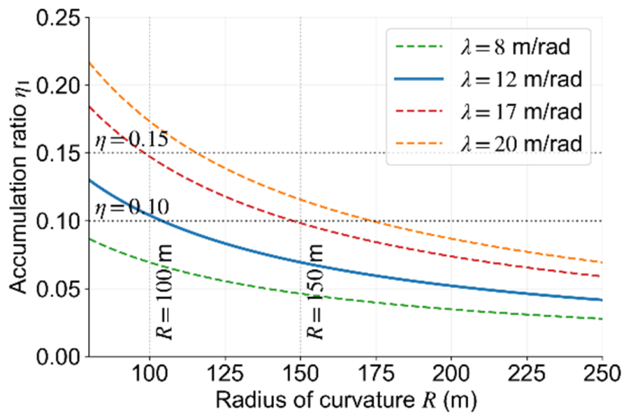
Figure 1 shows the η-R relationship for four values of λ: 8, 12, 17, and 20 m/rad. The value 17 m/rad is the direct back-calculation from Equation (15). The value 12 m/rad is the adopted value. The values 8 and 20 m/rad serve as lower and upper bounds. The reference lines at η = 0.10 and η = 0.15, and the boundary positions at R = 100 m and R = 150 m, are also marked.

The curve for λ = 17 m/rad passes through both calibration points. For λ = 12 m/rad, η ≈ 0.07 at R = 150 m, which is 30% below the 0.10 threshold. At R = 100 m, η ≈ 0.105, still below the 0.15 level. For λ = 8 m/rad, η ≈ 0.07 at R = 100 m, which appears overly optimistic. For λ = 20 m/rad, η approaches 0.12 at R = 150 m, leaving little room for practical design variation. We therefore select λ = 12 m/rad, which provides a practical balance and avoids imposing overly restrictive curvature constraints. The final choice is λ = 12 m/rad. It should be clarified that λ is treated as an engineering tuning parameter rather than a uniquely calibrated physical coefficient. Although λ = 17 m/rad is the formal mathematical best fit to the two calibration conditions, these conditions represent physically different states. The R = 150 m, η ≈ 0.10 condition corresponds to a relatively clean annulus, while R = 100 m, η ≈ 0.15 corresponds to an annular condition where significant accumulation has already developed. A single linear relation cannot perfectly represent both regimes, as the relationship between curvature and pressure loss becomes increasingly nonlinear once cuttings begin to accumulate. The adopted value λ = 12 m/rad provides a more responsive sensitivity to the onset of accumulation, which is physically reasonable for detecting the early stage of accumulation. This value should be recalibrated when field measurements become available.

The sensitivity of the recommended curvature radii to the empirical coefficients β and λ can be assessed from the model relationships. For Transition Zone I, R_min is given by Equation (29), which depends explicitly on λ. For the baseline condition θ = 36°, R_min ≈ 104 m. Varying λ from 10 to 14 m/rad changes R_min by approximately −17% to +17%. For Transition Zone II, R_min is influenced by β through the relationship η₂/η₁ = β·(R₁/R₂)², as shown in Equation (25). Varying β from 1.0 to 1.3 changes the required radii by approximately −7% to +6% relative to the baseline value obtained with β = 1.15. When both coefficients vary simultaneously over their full ranges, the combined effect on the recommended radii is approximately −24% to +23%. This range represents the worst-case bound; actual variations are likely to be smaller, but the reported interval indicates the maximum expected sensitivity to these empirical parameters.

3.2. Parametric Sensitivity Analysis

To compare the relative influence of different governing factors on the cuttings accumulation ratio, a sensitivity coefficient is defined as S_x = (∂η/∂x)⋅(x/η). All S_x values are calculated under the baseline condition of 36° inclination and R = 150 m.

From Equation (15), η is inversely proportional to R, which directly yields S_R = −1. Partial differentiation with respect to the annular return velocity v_l gives S_vl = −v_l/(v_l − v_cr) ≈ −1.76. The sensitivity to inclination angle θ is transmitted through the term v_cr(θ), and calculation using the gradient of the Larsen critical velocity near 36° gives S_θ ≈ 0.31. The resulting ranking of factor sensitivity is summarized in

Table 2. Sensitivity coefficients of each factor (baseline: θ = 36°, R = 150 m).

Factor	Sx	Description
Annular return velocity vl	−1.76	A 1% rise in vl reduces η by 1.76%
Curvature radius R	−1.00	A 1% rise in R reduces η by 1%
Wellbore inclination angle θ	0.31	A 1% rise in θ increases η by ~0.31%

.

As shown in Table 2, flow rate is the most sensitive parameter, followed by curvature radius, while inclination angle has the weakest effect. However, the practical range of flow-rate adjustment is limited by hole cleaning capacity and wellbore stability. Curvature radius optimization, though less sensitive, is more reliable. The ranking suggests a clear priority for field adjustments: first check the flow rate, then evaluate the curvature radius, and finally consider the inclination angle. If the inclination is high, compensation must still be provided by increasing the radius or the flow rate.

3.3. Effects of Inclination Angle and Curvature Radius

Equation (18) can be rewritten as

$${\eta }_1(R,\theta )=A(R)\cdot B(\theta )$$

(28)

where A(R) = λ·f(e)/R depends solely on the curvature radius, and B(θ) = v_cr(θ)/(v_l − v_cr(θ)) depends solely on the wellbore inclination angle. This formulation shows that the effects of R and θ on η₁ are fully separable, with no R-θ coupling term, so their respective influences on cuttings accumulation can be adjusted and analyzed independently.

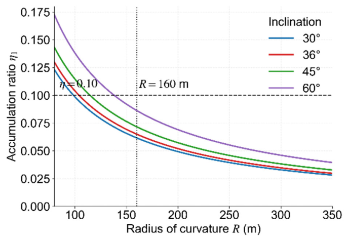
Figure 2 shows η₁ vs. R for four inclination angles. As Equation (18) implies, η₁ is inversely proportional to R at a fixed θ. All four curves decrease monotonically with increasing R. A higher inclination angle shifts the curve upward. At R = 160 m, η₁ = 0.062 at 30° and 0.070 at 60°, a difference of about 13%. The intersections with the η = 0.10 reference line give the minimum allowable curvature radii for each inclination angle. The values are 99 m, 104 m, 115 m, and 138 m for 30°, 36°, 45°, and 60°, respectively.

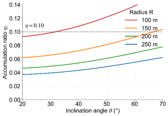
Figure 3 shows η₁ vs. θ for four curvature radii. At a fixed R, η₁ varies monotonically with v_cr(θ). According to the Larsen model, v_cr(θ) increases monotonically with θ over the range from 20° to 70°. All four curves therefore rise monotonically with θ, and a smaller curvature radius places the curve higher.

3.4. Effect of Flow Rate

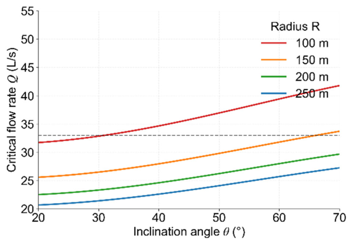
The flow rate Q enters through the annular velocity v_l. From Equation (15), increasing v_l increases the difference v_l − v_cr and thus reduces η. Figure 4 shows the minimum flow rate required to keep η₁ below 0.10 for different curvature radii.

All four curves increase monotonically with inclination. At R = 100 m, the required flow rate at 60° is about 39.6 L/s, 20% above the baseline of 33 L/s. At R = 150 m, the required rate at 60° is about 30.5 L/s, slightly below baseline. At R = 200 m and R = 250 m, the values are 27.1 L/s and 25.7 L/s, respectively. There is an equivalent substitution between R and Q: a smaller curvature radius can be partially offset by a higher flow rate.

3.5. Comparison of the Two Transition Zones

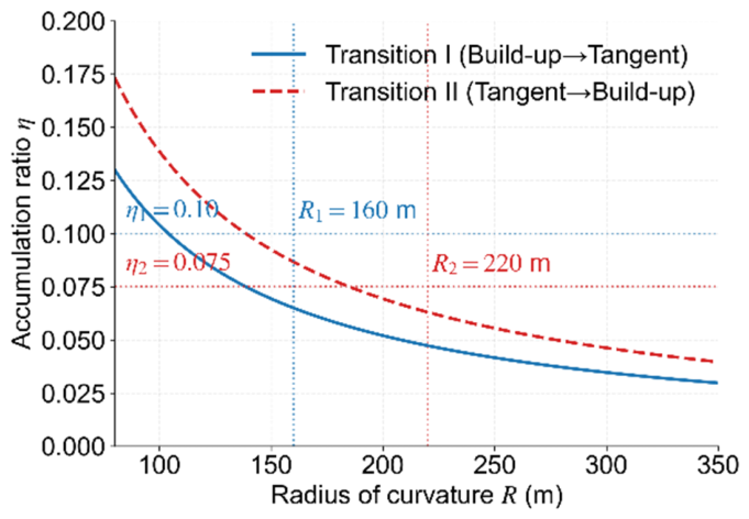
Figure 5 shows η₁ and η₂ vs. the curvature radius at θ = 36°. Here η₂ is computed from Equation (27) with the baseline condition R₁ = R₂ and ψ = 1.15. Both curves decrease monotonically with increasing R. The η₂ curve consistently lies above η₁. The difference narrows as R increases. It is 0.030 at R = 100 m and 0.012 at R = 250 m. A large curvature radius reduces the discrepancy between the two zones.

Using η = 0.10 and η = 0.075 as design limits gives R_1,min ≈ 105 m and R_2,min ≈ 140 m. The minimum radius for Transition Zone II is 33% higher than for Transition Zone I, reflecting the greater sensitivity of the secondary disturbance effect. Applying a safety factor of 1.5 yields recommended values of R₁ ≥ 160 m and R₂ ≥ 220 m.

Previous studies indicate that bed thickness tends to follow a consistent ranking across different sections of extended-reach wells: the build section exhibits the largest beds, followed by the horizontal, tangent, and vertical sections in decreasing order. Our results further show that even under the same build rate, a significant difference exists between the accumulation ratios at the end of the build section and at the end of the tangent section.

Figure 6 shows the variation in the dynamic disturbance amplification coefficient ψ and the accumulation ratios η₁ and η₂ of the two transition zones with the curvature radius ratio R₁/R₂. Here, η₁ remains constant because R₁ is fixed at 150 m, while η₂ decreases monotonically with increasing R₂ and thus decreases monotonically with increasing R₁/R₂. When R₂ = R₁, ψ = 1.15 and η₂/η₁ = 1.15. When R₂ > 1.072R₁, η₂/η₁ < 1, meaning the accumulation ratio in Transition Zone I exceeds that in Transition Zone II. When R₂ > 1.15R₁, ψ < 1, indicating that the secondary-flow disturbance intensity in Transition Zone II has fallen below that in Transition Zone I. This result demonstrates that the relative severity of the two transition zones is not fixed but depends on the designed curvature radii of the two segments.

3.6. Design Chart

The design chart combines the η = 0.10 boundary with the operational difficulty window. From Equation (18), the minimum allowable curvature radius R_min at η₁ = 0.10 is

$$R_{\min }={\displaystyle \frac{\lambda f(e)\cdot v_{cr}(\theta )}{0.10\cdot (v_l-v_{cr}(\theta ))}}$$

(29)

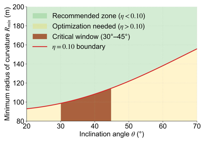
with λ = 12 m/rad, f(e) = 1.15, and v_l = 1.38 m/s, the values of R_min for 30°, 36°, 45°, and 60° are 99 m, 104 m, 115 m, and 138 m, respectively. Figure 7 plots these results.

The red curve marks the η = 0.10 boundary. The green region above the curve is the recommended operating zone; the yellow region below requires further optimization. In practice, the user reads the ordinate value on the curve for the target inclination angle θ, which gives the minimum curvature radius required to satisfy η = 0.10. If the actual radius exceeds this value, the design lies in the recommended zone. Otherwise, the flow rate should be increased or the trajectory adjusted.

In field practice, the curvature radius is often constrained by geological conditions, target locations, and anti-collision requirements, leaving limited room for adjustment. When the recommended minimum curvature radius cannot be achieved, the following engineering measures can be considered as compensatory strategies to mitigate cuttings accumulation:

(1)

Optimizing drilling fluid rheology: Increasing the fluid’s yield stress and low-shear viscosity can enhance the carrying capacity of the annular flow and reduce cuttings settling.

(2)

Increasing drill pipe rotation speed: The helical flow induced by pipe rotation can disturb the cuttings bed and promote particle re-entrainment.

(3)

Deploying mechanical bed-breaking tools: Specialized tools that combine hydraulic and mechanical actions can effectively break and disperse the cuttings bed.

These measures can be implemented individually or in combination, depending on the specific operational constraints and cost considerations. The design chart provides a baseline reference; the actual operating parameters should be determined through integrated evaluation of the above factors.

The recommended minimum curvature radii R₁ ≥ 160 m and R₂ ≥ 220 m are derived under the specific assumptions of this study: water-based mud with rheological properties as listed in Table 1, a 215.9 mm wellbore, a 127.0 mm drill pipe, and field data from the Jidong Oilfield of PetroChina. Sensitivity analysis with respect to the empirical coefficients β and λ is presented in Section 3.1.2. The analysis shows that varying β from 1.0 to 1.3 and λ from 10 to 14 m/rad changes the recommended radii by approximately −24% to +23% when both coefficients vary simultaneously over their full ranges, representing the worst-case bound of the sensitivity to these empirical parameters. These values should be treated as condition-specific engineering guidelines rather than universally validated limits and should be adjusted for different wellbore sizes, drilling fluid systems, and formation conditions.

4. Discussion

The two transition zones differ in the direction of the abrupt flow-field change. In Transition Zone I, curvature decreases from a finite value to zero, and secondary-flow decays. In Transition Zone II, curvature increases from zero to a finite value, and secondary flow is suddenly generated. Earlier studies typically treated the entire build section as a single unit when comparing it with the tangent section and did not examine local accumulation within the build segment itself. Our results show that accumulation severity differs systematically between the end of the build section and the end of the tangent section—accumulation concentrates at the curvature-change location rather than being distributed uniformly over the entire build section.

The value β = 1.15 is based on experimental data. The ratio of secondary-flow decay length to development length in curved pipes ranges from 1.2 to 1.5 [15]. We take the lower end of this range as a provisional choice in the absence of directly applicable annular-flow data, with its quantitative validity subject to future validation. The review by Saffar et al. [17] supports the use of the Dean number gradient as the governing quantity for disturbance intensity. This justifies our use of dDe_pl/ds. The relation η₂/η₁ = β·(R₁/R₂)² explicitly describes how the relative severity of the two zones depends on the chosen curvature radii. When R₂ > 1.072R₁, Transition Zone I becomes the critical condition.

Compared with the three-layer models of Guo et al. [4] and Nguyen and Rahman [14], our work introduces the curvature radius as an independent variable. We use ψ to quantify the dynamic effect of the curvature-change rate. The three-layer transient model of Al Rubaii et al. [21] and the wavy-bed analysis of Zhu et al. [18] both confirm that trajectory geometry matters. However, neither addresses the local difference at curvature mutation points. Our design chart allows direct reading of the minimum curvature radius for a given inclination. The sensitivity ranking is flow rate, curvature radius, and inclination angle. This provides a clear guide for field decisions. Curvature radius optimization is more reliable than flow-rate adjustment. Transition Zone II is usually the governing condition. When R₂ > 1.072R₁, Transition Zone I becomes more severe. This crossover should be noted in design.

The main limitation of the present model is that inter-layer mass exchange and transient operational effects are neglected, and the coefficient λ requires recalibration for different wellbore sizes. Zhang et al. [22] pointed out that dynamic cuttings transport and drill string mechanical behavior are mutually coupled, and traditional independent research can no longer meet the practical engineering requirements. Erge et al. [23] validated the effects of eccentricity and drill pipe rotation on cuttings transport in non-Newtonian fluids via CFD simulations, confirming that the curvature-induced eccentricity effect is a key factor governing accumulation. However, their work still did not couple this effect with the local flow disturbance at the transition zone curvature mutation points. The analytical framework and sensitivity ranking proposed in this work are of general applicability, while the specific values of λ and ψ still need to be calibrated according to the actual wellbore conditions.

5. Conclusions

(1)

Based on the three-layer cuttings transport model, we derived analytical expressions for the accumulation ratio in the two curvature transition zones and introduced a curvature correction term λ/R to account for the effect of build-section curvature on the critical transport velocity. For power-law fluids, a generalized Reynolds number was used to modify the Dean number, and a dynamic disturbance amplification factor ψ was constructed from the streamwise gradient of the Dean number to quantify the accumulation difference caused by opposite curvature-change directions in the two transition zones.

(2)

A systematic difference exists between the two transition zones. When R₁ = R₂, η₂/η₁ = ψ = β ≈ 1.15, indicating that Transition Zone II carries a higher accumulation risk. When R₂ > 1.072R₁, η₂/η₁ < 1, and Transition Zone I becomes the governing condition. The relative severity is determined by the designed curvature radii.

(3)

Reducing the curvature radius from 250 m to 100 m increases the accumulation ratio by about 2.5 times. We recommend minimum curvature radii of R₁ ≥ 160 m for the first build section and R₂ ≥ 220 m for the second. These values are condition-specific and should be adjusted for different wellbore sizes, drilling fluid systems, and formation conditions. At the commonly used build rate of 6°/30 m (corresponding to R ≈ 286 m), the accumulation ratio remains far below the design limit, providing ample cleaning margin.

(4)

The accumulation ratio increases with inclination angle. There is no local peak under the Larsen model. The sensitivity ranking is flow rate, curvature radius, and inclination angle. Curvature radius optimization is more reliable than flow-rate adjustment. If the allowable radius is limited, a moderate increase in flow rate can serve as compensation.

The model neglects interlayer mass exchange and transient effects. The coefficient λ must be recalibrated for different wellbore sizes. Nevertheless, the analytical framework and sensitivity ranking are generally applicable.

References

1. Doron, P.; Barnea, D. A three-layer model for solid-liquid flow in horizontal pipes. Int. J. Multiph. Flow 1993, 19, 1029–1043. [Google Scholar] [CrossRef] [Scilit]
2. Liu, X.; Zheng, X.; Ding, G. Study on prediction model of cuttings bed thickness in highly deviated wells. J. China Univ. Pet. (Ed. Nat. Sci.) 1991, 15, 28–35. [Google Scholar]
3. Martins, A.; Santana, M.; Campos, W. Evaluating the transport of solids generated by shale instabilities in ERW drilling. SPE Drill. Complet. 1999, 14, 254–259. [Google Scholar] [CrossRef] [Scilit]
4. Guo, X.; Wang, Z.; Long, Z. Dynamic cuttings transport law in full hole interval of extended reach drilling. J. China Univ. Pet. (Ed. Nat. Sci.) 2011, 35, 72–76. [Google Scholar]
5. Zhao, J.; Huang, W.; Gao, D. Coupling analysis of transient cuttings transport and tubular mechanical behaviors in extended-reach drilling. Pet. Sci. 2025, 22, 1252–1269. [Google Scholar] [CrossRef] [Scilit]
6. Larsen, T.; Pilehvari, A.; Azar, J. Development of a new cuttings-transport model for high-angle wellbores including horizontal wells. SPE Drill. Complet. 1997, 12, 129–135. [Google Scholar] [CrossRef] [Scilit]
7. Larsen, T. A Study of the Critical Fluid Velocity in Cuttings Transport for Inclined Wellbores. Master’s Thesis, The University of Tulsa, Tulsa, OK, USA, 1990. [Google Scholar]
8. Yang, S.; Zhang, J.; Shen, J. Experimental study on cuttings carrying law of drilling fluid in highly deviated wells. J. Daqing Pet. Inst. 1997, 21, 126–129. [Google Scholar]
9. Li, Y.; Wen, K.; Li, G. Influence of drill pipe eccentricity on annular cuttings transport law in gas drilling horizontal wells. Sci. Technol. Eng. 2016, 16, 35–41. [Google Scholar]
10. Sun, X.; Ji, G.; Wang, K. Influence of drill string rotation on cuttings transport in highly deviated eccentric annulus. Spec. Oil Gas Reserv. 2015, 22, 133–136. [Google Scholar]
11. Li, M.; Wang, Z.; Hao, B. Study on influence of drill string rotation on hole cleaning in extended reach wells. China Pet. Mach. 2009, 37, 34–37. [Google Scholar]
12. Ofei, T. Effect of yield power law fluid rheological properties on cuttings transport in eccentric horizontal narrow annulus. J. Fluids 2016, 2016, 4931426. [Google Scholar] [CrossRef] [Scilit]
13. Zheng, X.; Liu, X.; Ding, G. Study on cuttings transport mechanism in annulus of directional wells. J. China Univ. Pet. (Ed. Nat. Sci.) 1991, 15, 25–31. [Google Scholar]
14. Nguyen, D.; Rahman, S. A three-layer hydraulic program for effective cuttings transport and hole cleaning in highly deviated and horizontal wells. SPE Drill. Complet. 1998, 13, 182–189. [Google Scholar] [CrossRef] [Scilit]
15. Kim, W.; Patel, V. Origin and decay of longitudinal vortices in developing flow in a curved rectangular duct (data bank contribution). J. Fluids Eng. 1994, 116, 45–52. [Google Scholar] [CrossRef] [Scilit]
16. Dean, W. Note on the motion of fluid in a curved pipe. Philos. Mag. 1927, 4, 208–223. [Google Scholar] [CrossRef] [Scilit]
17. Saffar, Y.; Kashanj, S.; Nobes, D. The physics and manipulation of Dean vortices in single- and two-phase flow in curved microchannels: A review. Micromachines 2023, 14, 2202. [Google Scholar] [CrossRef] [Scilit] [PubMed]
18. Zhu, N.; Huang, W.; Gao, D. Dynamic wavy distribution of cuttings bed in extended reach drilling. J. Pet. Sci. Eng. 2021, 198, 108171. [Google Scholar] [CrossRef] [Scilit]
19. Jing, S.; Song, X.; Zhou, M. Experimental investigation of the annular cross-sectional distribution of cuttings bed with drillpipe rotation in horizontal wells. Powder Technol. 2024, 436, 119520. [Google Scholar] [CrossRef] [Scilit]
20. Xue, M.; Hou, J.; Li, Z. Cuttings transport model and experimental study for multilateral horizontal wells. Drill. Eng. 2024, 51, 31–39. [Google Scholar]
21. Al-Rubaii, A.; Al-Maamari, A.; Al-Maamari, M. Three-layer nonstationary model of cuttings transport in oil wells. J. Pet. Sci. Eng. 2023, 227, 112045. [Google Scholar]
22. Zhang, F.; Wang, Y.; Wang, Y. Modeling of dynamic cuttings transportation during drilling of oil and gas wells by combining 2D CFD and 1D discretization approach. SPE J. 2020, 25, 1220–1240. [Google Scholar] [CrossRef] [Scilit]
23. Erge, O.; Ozbayoglu, E.; May, R. CFD modelling of observed cuttings transport in oil-based and water-based drilling fluids. SPE J. 2016, 21, 1789–1801. [Google Scholar]
Figure 1. Variation in η1 with R for different λ at θ = 36°.
Fluids 11 00230 g001
Figure 2. Accumulation ratio vs. curvature radius for different inclination angles.
Fluids 11 00230 g002
Figure 3. Accumulation ratio vs. inclination angle for different curvature radii.
Fluids 11 00230 g003
Figure 4. Critical flow rate vs. inclination angle for different curvature radii (η1 = 0.10).
Fluids 11 00230 g004
Figure 5. Comparison of accumulation ratios for the two transition zones (θ = 36°).
Fluids 11 00230 g005
Figure 6. Variation in dynamic disturbance amplification coefficient ψ and accumulation ratios η1, η2 with curvature radius ratio R1/R2 (β = 1.15, R1 = 150 m).
Fluids 11 00230 g006
Figure 7. Design chart for optimized trajectory.
Fluids 11 00230 g007