Multi-Objective Optimization of a Rotary Vane Vacuum Pump for Vapor Recovery Based on PSO

Abstract

The rotary vane vacuum pump plays a key role in the vapor recovery process at gasoline stations, where its geometric configuration directly influences system efficiency and stability. To address the limitations of conventional designs, this study develops a multi-objective optimization framework using particle swarm optimization (PSO). Under fixed chamber dimensions and specified constraints, the optimal design parameters are identified. The optimized pump achieves a 12.8% increase in average theoretical flow rate over the reference pump. Correlation analysis reveals that the exhaust port start angle has the strongest influence on performance, exhibiting a trade-off between compressed chamber pressure and exhaust pulsation. The rotor radius shows strong negative correlations with all objectives, while the intake port end angle is found to be a redundant parameter. Constraint sensitivity analysis indicates that the rotor radius and exhaust port start angle respond stably to variations in key constraints. Numerical simulations confirm a well-matched exhaust process, with the exhaust pulsation ratio minimized at an exhaust port start angle of 235°. This systematic approach provides an effective methodology for enhancing pump performance while respecting geometric constraints.

1. Introduction

Gasoline, a complex mixture of highly volatile C₄–C₁₂ hydrocarbons, continuously releases volatile organic compounds (VOCs) during vehicle refueling [1,2]. These emissions not only result in substantial resource waste but also pose threats to air quality and public health [3,4,5]. The refueling process is particularly critical for VOC emissions because liquid gasoline entering the tank displaces the existing vapor–air mixture, and the high-velocity, turbulent flow significantly accelerates vapor generation, leading to concentrated releases in a short period. Consequently, controlling vapor emissions during vehicle refueling has become a priority in air pollution prevention strategies worldwide.

To capture the fugitive vapors generated during refueling, Stage II Vapor Recovery systems are widely employed. These systems establish a sealed connection between the nozzle and the vehicle fuel tank, using vacuum assistance to simultaneously return the displaced vapor to the underground storage tank, thereby forming a closed-loop cycle that reduces VOCs at the source [6,7]. Within this system, the vacuum pump serves as the core power unit, and its performance directly determines the efficiency and reliability of vapor recovery [8].

The vacuum pump must generate sufficient negative pressure to overcome flow resistance in the piping and maintain a stable air-to-liquid ratio (ALR). The ALR is a key efficiency indicator, requiring the recovered vapor volume to closely match the dispensed fuel volume, typically regulated between 0.95 and 1.05 [9,10]. The stability of the ALR not only affects the VOCs capture rate but also directly impacts regulatory compliance. Therefore, the vacuum pump must possess the capability for stable output and dynamic adjustment across a wide operating range.

Among various vacuum pump technologies, the rotary vane pump has emerged as the dominant choice for vapor recovery applications due to its distinct advantages. Its operating principle is based on the interaction between an eccentrically mounted rotor and radially sliding vanes: the vanes, pressed against the chamber wall by centrifugal forces, create multiple sealed working chambers that undergo cyclic volume changes, enabling continuous intake and exhaust [11]. Compared to other pump types, the rotary vane pump offers a compact structure, high power density, low operating noise, and excellent reliability, making it particularly suitable for the space-constrained environment of fuel dispensers [12].

However, the operating conditions in vapor recovery impose unique requirements on the rotary vane pump, distinguishing it from traditional high-vacuum applications. Conventional rotary vane pumps are designed for achieving ultimate vacuum in sealed systems, prioritizing ultimate vacuum level and low backflow rates [13,14]. In contrast, vapor recovery pumps operate with inlet pressures near atmospheric levels, and their primary requirement is sustained high volumetric flow rate rather than ultimate vacuum. Furthermore, refueling rates vary considerably depending on vehicle type and operator behavior, necessitating that the pump possesses dynamic flow regulation capability to maintain a stable ALR [15]. These unique operating conditions render the design theories and methods of traditional rotary vane pumps largely inapplicable unless modified.

More critically, the current design of vapor recovery pumps still relies heavily on empirical experience, lacking a systematic optimization framework. Geometric parameters such as rotor radius, eccentricity, vane number, and intake/exhaust port positions are highly coupled; adjusting one parameter in isolation often leads to trade-offs in performance [16,17]. Additionally, the transient flow dynamics inside the pump involve complex transcendental equations, making it difficult to express key performance indicators as explicit functions of the design variables, thus rendering traditional gradient-based optimization methods ineffective [18]. This methodological gap hinders further improvements in pump energy efficiency and reliability, making multi-objective optimization an essential approach in pump design [19].

Particle swarm optimization (PSO) and its variants have been widely adopted in pump optimization due to their simplicity, fast convergence, and strong global search capability. In axial-flow pumps, Miao et al. [20] and Park and Miao [21] combined a modified PSO with a GMDH neural network to simultaneously improve efficiency and cavitation performance. Li [22] further integrated design of experiments, response surface methodology, and PSO to optimize groove flow control structures in an axial-flow pump, significantly enhancing hydraulic performance under stall conditions. For centrifugal pumps, Pei et al. [23] and Wang et al. [24] used artificial neural networks to establish nonlinear mappings between impeller design variables and performance targets, and then solved the optimization problem using PSO. Bashiri [25] adopted a similar ANN-PSO strategy, achieving a 3.2% efficiency increase and a 5.52 m head rise.

To reduce the high computational cost of direct optimization, surrogate-assisted PSO frameworks have been developed. Fang et al. [26] combined PSO with least-squares support vector regression (LSSVR) to optimize a centrifugal pump impeller. Lin [27] applied a PSO-LSSVR surrogate model to a multistage LNG cryogenic pump, achieving a 0.57% head increase and a 2.72% efficiency improvement with prediction errors below 3%. They further used PSO-LSSVR for a hydrogenation feed pump [28], obtaining a 3.99% head rise and a 2.91% efficiency gain, while energy loss decreased by 9% at the rated condition. In comparison, Gan et al. [29] performed a direct multi-objective PSO (MOPSO) optimization on 39 geometric parameters of an inline pump using over 7000 samples. Although computationally intensive, this direct approach achieved an impressive efficiency improvement of up to 8.06%.

The above studies indicate that surrogate-assisted PSO methods are widely used in pump optimization. These methods approximate the objective function by constructing surrogate models, such as response surfaces, neural networks, or Kriging, based on sampled data [30]. However, the prediction accuracy of a surrogate model is limited by the distribution and number of sample points, leading to non-negligible errors. More importantly, as the number of design parameters increases, the required sample size grows exponentially, which severely restricts the applicability of surrogate-assisted PSO to multi-parameter, high-precision optimization problems [31].

To address the aforementioned challenges, this study does not construct a surrogate model. Instead, it directly integrates a theoretical model of the rotary vane vacuum pump with a multi-objective PSO algorithm. Based on this framework, the optimal geometric parameters are obtained under fixed chamber dimensions and key constraints. Correlation analysis and constraint sensitivity analysis are conducted to interpret the optimization results, and numerical simulations are performed to evaluate the optimized design. The results provide a theoretical and methodological basis for the systematic design of high-efficiency vapor recovery vacuum pumps.

2. Methods

2.1. Theoretical Model

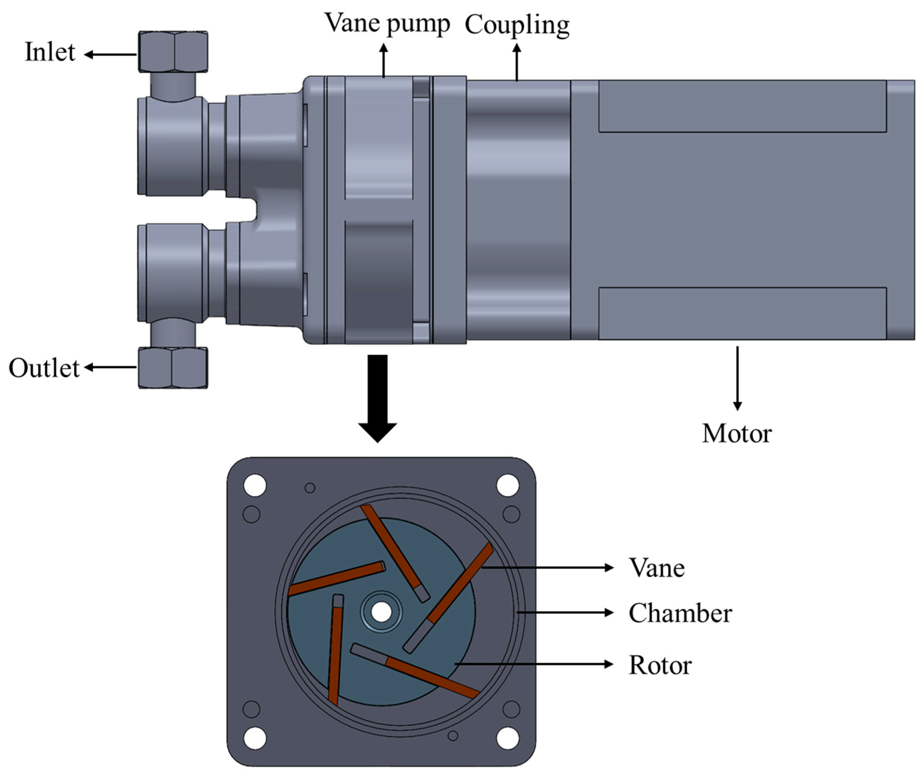
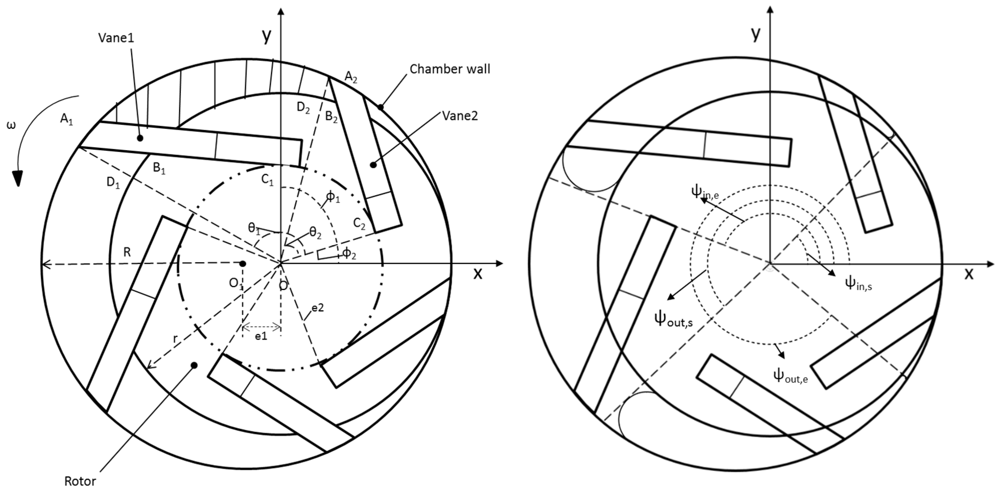
The structure of the rotary vane vapor recovery pump is shown in Figure 1. Based on this structure, the geometric model of the pump is established in Figure 2, where the shaded area represents the elemental area to be calculated. The rotor rotates counterclockwise around its center O with a radius of r; the pump chamber center is O₁, with a radius of R. The offset distance between the rotor center and the pump chamber center is e₁; the vane eccentricity is e₂; and the vane thickness is B. A planar Cartesian coordinate system is established with the rotor center point O as the origin and the direction O₁O as the positive x-axis. The initial position of the rotor is defined when OC₁ coincides with the x-axis. The positions of the pump’s intake and exhaust ports are determined by the intake port start angle (ψ_in,s), intake port end angle (ψ_in,e), exhaust port start angle (ψ_out,s), and exhaust port end angle (ψ_out,e).

The vane polar radius is given by:

$$\rho =e_1\mathrm{c}\mathrm{o}\mathrm{s}\theta +\sqrt{R^2-e_1^2{\sin }^2\theta }$$

The relationship between the vane polar angle θ and the rotor rotation angle φ is:

$$\theta =\alpha +\phi -\arcsin {\displaystyle \frac{e_2\mathrm{s}\mathrm{i}\mathrm{n}\alpha }{\rho }}$$

where α is the angle between the vane and the rotor slot.

The vane extension length L_AB is:

$$L_{\mathrm{A}\mathrm{B}}=L_{\mathrm{A}\mathrm{C}}-L_{\mathrm{B}\mathrm{C}}=\sqrt{{\rho }^2{-e}_2^2{\sin }^2\alpha }-\sqrt{r^2-e_2^2{\sin }^2\alpha }$$

The elementary chamber area, S_O, is defined as the cross-sectional area of the elementary chamber on a plane perpendicular to the stator axis, i.e., the shaded area in Figure 1. For a rotary vane pump with z vanes, the angular interval between adjacent vanes is Δφ = 2π/z. The front vane of the elementary chamber is denoted as vane 1 with an angular position of φ₁; the rear vane is denoted as vane 2 with an angular position of φ₂. Let φ₁ = φ, then

$$\phi ={\phi }_1-\nabla \phi =\phi -{\displaystyle \frac{2\pi }{z}}$$

Based on the geometric relationships, the expression for S_O can be derived as:

$$S_{\mathrm{O}}=S_{\mathrm{O}{\mathrm{A}}_1{\mathrm{A}}_2}+S_{{\mathrm{A}}_2{\mathrm{B}}_2{\mathrm{D}}_2}-S_{0{\mathrm{D}}_1{\mathrm{D}}_2}-S_{{\mathrm{A}}_1{\mathrm{B}}_1{\mathrm{D}}_1}-S_1$$

S_OA1A2 is the area enclosed by the polar radii OA₁ and OA₂ and the arc A₁A₂:

$$S_{{\mathrm{O}\mathrm{A}}_1{\mathrm{A}}_2}={\int }_{{\theta }_2}^{{\theta }_1}{\displaystyle \frac{1}{2}}{\rho }^2\mathrm{d}\theta$$

where $\epsilon ={\displaystyle \frac{e_1}{R}}$ is the relative eccentricity of the rotor.

S_OD1D2 is the area enclosed by the radii OD₁ and OD₂ and the arc D₁D₂:

$$S_{\mathrm{O}{\mathrm{D}}_1{\mathrm{D}}_2}={\displaystyle \frac{1}{2}}\left({\theta }_1-{\theta }_2\right)r^2$$

S_A1B1D1 is the area enclosed by the line segments A₁B₁ and A₁D₁ and the arc B₁D₁:

$$S_{{\mathrm{A}}_1{\mathrm{B}}_1{\mathrm{D}}_1}={\displaystyle \frac{1}{2}}{e}_2{L}_{{\mathrm{A}}_1{\mathrm{B}}_1}\mathrm{s}\mathrm{i}\mathrm{n}\alpha -{\displaystyle \frac{1}{2}}{\beta }_1{r}^2$$

where β₁ is the central angle subtended by the arc B₁D₁:

$${\beta }_1=\arccos \left({\displaystyle \frac{{\rho }_1^2+r^2-L_{{\mathrm{A}}_1{\mathrm{B}}_1}^2}{2{\rho }_{1}r}}\right)$$

S_A2B2D2 is the area enclosed by the line segments A₂B₂ and A₂D₂ and the arc B₂D₂:

$$S_{{\mathrm{A}}_2{\mathrm{B}}_2{\mathrm{D}}_2}={{\displaystyle \frac{1}{2}}e}_2{L}_{{\mathrm{A}}_2{\mathrm{B}}_2}\mathrm{s}\mathrm{i}\mathrm{n}\alpha -{\displaystyle \frac{1}{2}}{\beta }_2{r}^2$$

where β₂ is the central angle subtended by the arc B₂D₂:

$${\beta }_2=\arccos \left({\displaystyle \frac{{\rho }_2^2+r^2-L_{{\mathrm{A}}_2{\mathrm{B}}_2}^2}{2{\rho }_{2}r}}\right)$$

The effective cross-sectional area occupied by the vane, S₁, is:

$$S_1=B{L}_{{\mathrm{A}}_1{\mathrm{B}}_1}$$

By integrating the above formulas, the elemental area S₀ of the vapor recovery vacuum pump can be calculated. Given the pump chamber height H, the elemental volume is obtained as:

$$V=S_{0}H$$

(1)

The total elemental volume currently connected to the outlet port can be found by summing the individual elemental volumes connected to the outlet:

$$V_{\mathrm{o}\mathrm{u}\mathrm{t}}=\sum V_i$$

(2)

where V_i represents an elemental volume connected to the outlet.

The instantaneous flow rate at the outlet port is defined as the rate of change of the total elemental volume connected to the outlet:

$$Q_{\mathrm{o}\mathrm{u}\mathrm{t}}={\displaystyle \frac{\mathrm{d}{V}_{\mathrm{o}\mathrm{u}\mathrm{t}}}{\mathrm{d}t}}$$

(3)

The time-averaged outlet flow rate is obtained by averaging the instantaneous flow rate over time:

$$Q_{\mathrm{a}\mathrm{v}\mathrm{e}}={\displaystyle \frac{{\displaystyle {\int }_0^T}{Q}_{\mathrm{o}\mathrm{u}\mathrm{t}}\mathrm{d}\mathrm{t}}{T}}$$

(4)

where T is the vane rotation period.

The exhaust pulsation characteristic of the vacuum pump is quantified by the exhaust pulsation ratio:

$$\delta ={\displaystyle \frac{\mathrm{M}\mathrm{a}\mathrm{x}\left(Q_{\mathrm{o}\mathrm{u}\mathrm{t}}\right)-\mathrm{M}\mathrm{i}\mathrm{n}\left(Q_{\mathrm{o}\mathrm{u}\mathrm{t}}\right)}{Q_{\mathrm{a}\mathrm{v}\mathrm{e}}}}$$

(5)

2.2. Optimization Methodology

This study presents the optimal design of a rotary vane vacuum pump to maximize the outlet flow rate and minimize the exhaust pulsation ratio, formulating the task as a multi-objective, multi-parameter optimization problem:

$$\{\begin{array}{c}\min F\left(X\right)=[f_1\left(X\right),f_2\left(X\right),\dots ]\\ s.t. { g}_j\left(X\right)\le 0 j=\mathrm{1,2},\dots ,m\\ x_i^{\mathrm{m}\mathrm{i}\mathrm{n}}\le x_i\le x_i^{\mathrm{m}\mathrm{a}\mathrm{x}} i=\mathrm{1,2},\dots ,n\end{array}$$

(6)

where X = (x₁, x₂, …, x_n) represents the vector of design variables: x₁ = r, x₂ = e₂, x₃ = z, x₄ = ψ_in,e, and x₅ = ψ_out,s. The functions f₁(X) and f₂(X) denote the pump’s average outlet flow rate and exhaust pulsation ratio, respectively. The constraints are given by g_j(X) ≤ 0 (j = 1, 2, …, m), where m is the number of constraints. The lower and upper bounds for each variable x_i are x_i^min and x_i^max, respectively, and n is the dimension of the design variable space. As the number of vanes (x₃) is an integer variable, it is rounded down during the optimization process. The key geometric parameters of the reference pump are as follows: chamber radius of 33 mm, rotor radius of 29 mm, 5 vanes (each 3 mm thick), intake port end angle of 144°, and exhaust port end angle of 216°. To control the pump size for easier installation inside the fuel dispenser, the pump chamber dimensions are fixed at a radius of 30 mm and a height of 25 mm during optimization. The ranges of the optimization variables are listed in

Table 1. Bounds of the optimization variables.

Variable	Unit	Lower Bound	Upper Bound
x1	mm	18.5	27.5
x2	mm	8	20
x3	/	3	7
x4	°	130	160
x5	°	200	250

.

The constraint conditions are determined based on the following considerations:

(1) To ensure proper pump operation, the vane must fully retract into its slot at the rotor-stator contact point. This requires that the vane length be less than the slot length; furthermore, to ensure smooth sliding and effective sealing, the maximum vane extension $L_{\mathrm{AB}}^{\max }$ should not exceed λ times the vane length.

$$g_1\left(X\right)=L_{\mathrm{A}\mathrm{B}}^{\mathrm{m}\mathrm{a}\mathrm{x}}-\mathsf{\lambda }(\sqrt{r^2{-e}_2^2}+e_2\mathrm{t}\mathrm{a}\mathrm{n}({\displaystyle \frac{2\pi }{z}})-\sigma )\le 0$$

(7)

Here, σ is a safety distance between adjacent vane slots, and to maintain rotor structural integrity, σ = 12 mm. λ is the vane extension factor, λ = 0.6.

(2) To minimize energy consumption and compression temperature rise while ensuring the collected gas flows into the storage tank, the exhaust pressure of each compression chamber should match the tank pressure at the end of compression.

$${g_2\left(X\right)=P_{\mathrm{t}\mathrm{a}\mathrm{n}\mathrm{k}}-P}_{\mathrm{c}}=0$$

(8)

where P_tank is the tank pressure, and P_c is the pressure in the compression chamber at the beginning of discharge, as follows:

$$P_{\mathrm{c}}{=P}_{\mathrm{i}\mathrm{n}}{\left({\displaystyle \frac{V_{max}}{V_{\mathrm{c}}}}\right)}^k$$

(9)

where P_in denotes the inlet pressure, V_max represents the maximum chamber volume at the end of suction, V_c is the elemental volume of the compression chamber at the beginning of discharge, and k is the isentropic exponent (k = 1.3).

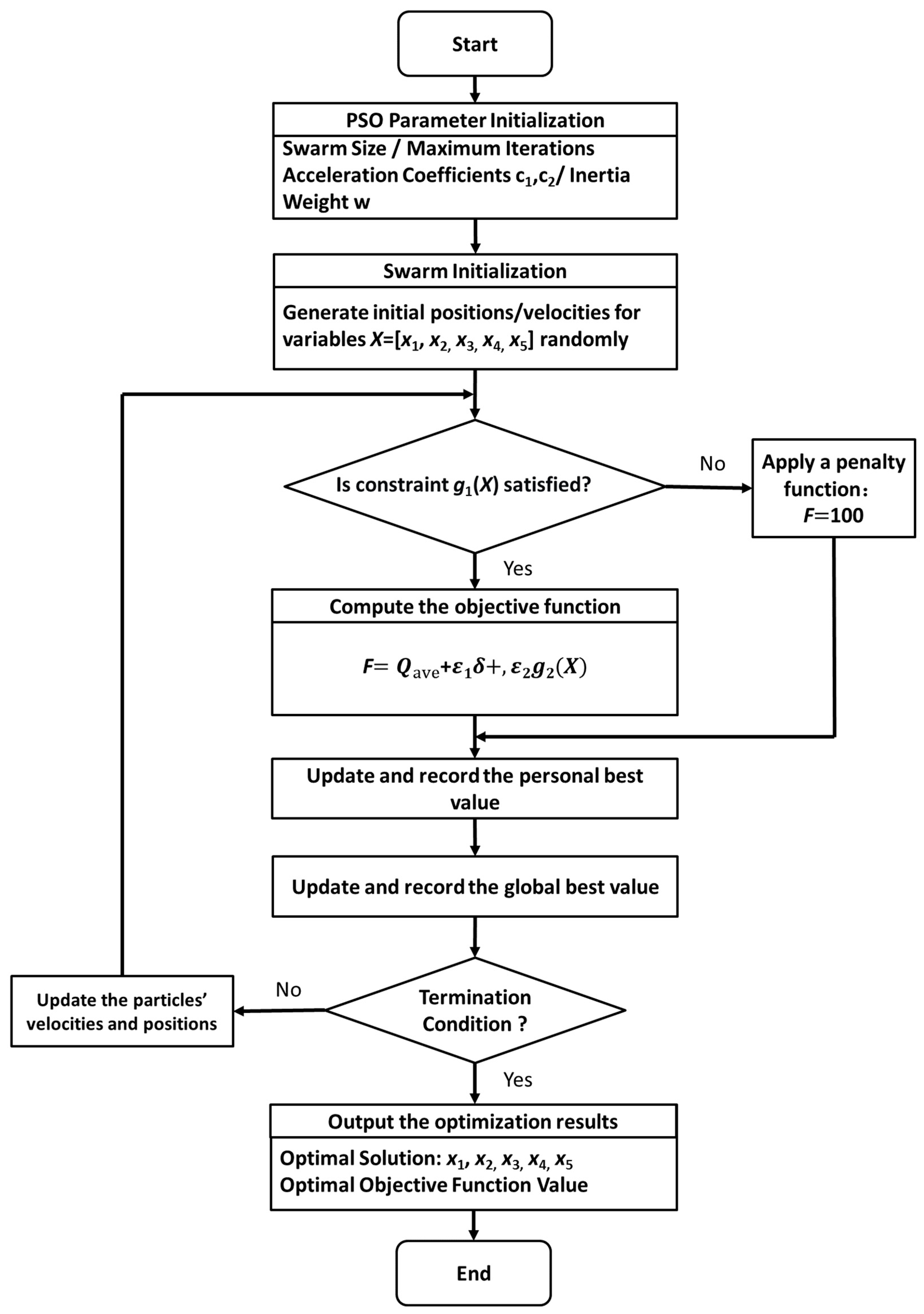
This optimization problem involves transcendental equations, making an explicit objective function formulation impossible. Therefore, the PSO algorithm was employed for its rapid convergence, straightforward parameter tuning, and strong global search capability [32]. The workflow of the optimization process is shown in Figure 3, with the values of the key PSO parameters, which are typical and widely used in PSO applications, listed in

Table 2. The parameters of PSO.

Parameter	Value
Number of particles	50
Dimension	5
Acceleration coefficient 1	2
Acceleration coefficient 2	2
Initial inertia weight	0.9
Final inertia weight	0.4

.

The three objectives differ substantially in magnitude. Q_ave is on the order of tens, δ is on the order of 0.1, and g₂(X) is on the order of hundreds to thousands. To ensure that no single objective dominates the optimization process, the weights are chosen to equalize their contributions to the scalar objective function. Specifically, the weight ε₁ for δ was set to 100 and ε₂ for g₂(X) to 0.01, while Q_ave was left unweighted as the primary objective. This brings the weighted terms to comparable orders of magnitude, enabling a balanced multi-objective optimization.

2.3. Numerical Model

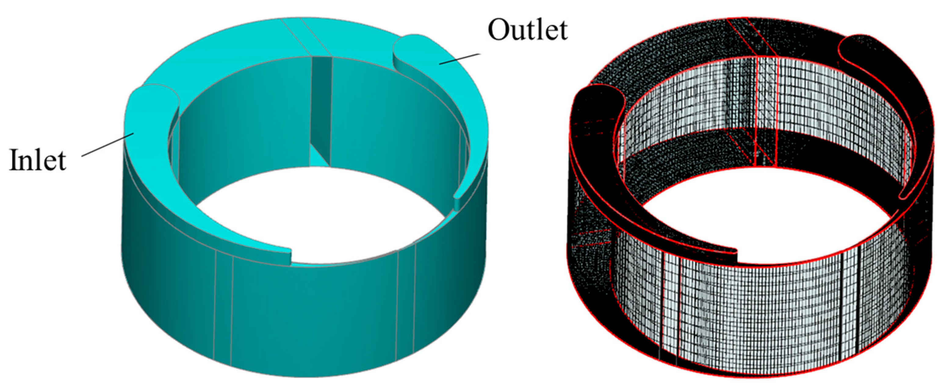
A three-dimensional numerical model of the optimized rotary vane pump was developed in PumpLinx v4.6.0 to analyze the transient flow characteristics, including the instantaneous outlet flow rate and internal pressure distributions. The fluid domain was created comprising the pump chamber and the inlet/outlet regions, with the vanes excluded; the inlet and outlet ports have an axial height of 3 mm. A structured hexahedral mesh was generated for the rotor and port regions. The fluid domain model and mesh are shown in Figure 4. The simulation assumed an adiabatic compression process and used air as the working medium, with a dynamic viscosity of 1.853 × 10⁻⁵ Pa·s, a thermal conductivity of 0.7 W/(m·K), and a specific heat capacity of 1005 J/(kg·K). Inlet and outlet pressure boundary conditions of 101.325 kPa and 103.825 kPa were applied, respectively. The rotor speed was set to 1500 rpm.

In the simulation, the governing equations for mass, momentum, and energy were discretized using the finite volume method (FVM), with the first-order upwind scheme employed for convective terms. Turbulence was modeled using the standard k-ε approach. The pressure–velocity coupling was handled by the SIMPLES algorithm, an improved variant of the SIMPLE method. The velocity and pressure linear systems were solved using the CGS and AMG iterative solvers, respectively, with a maximum of 50 sweeps and a linear solver tolerance of 0.1. Automatic relaxation was employed with a diagonal relaxation factor of 0.3 for both velocity and pressure. The convergence criterion was set to 0.1. Time integration was performed using a first-order implicit scheme, chosen for its numerical stability and computational efficiency. The simulation covered 4 complete revolutions, employing a time step of 4 × 10⁻⁴ s with 50 iterations per time step.

A systematic grid independence verification was conducted to ensure that the numerical results are not significantly influenced by spatial discretization. Three mesh sets with different levels of refinement, designated as coarse, medium, and fine, were generated for the computational domain of the gasoline vapor recovery vacuum pump. The corresponding surface mesh sizes were set to 5 mm, 2.5 mm, and 1.25 mm, resulting in total cell counts of approximately 163,300, 232,384, and 327,526 elements, respectively. The average volumetric flow rate was selected as the key monitoring parameter for the grid sensitivity assessment. The predicted flow rates obtained from the coarse, medium, and fine meshes are 57.0 L/min, 56.5 L/min, and 57.0 L/min, respectively. The maximum deviation among the three mesh schemes is less than 1%, indicating that the numerical solution is essentially grid-independent. Considering both computational accuracy and efficiency, the medium mesh scheme with 232,384 elements was therefore adopted for all subsequent numerical simulations in this study.

2.4. Experimental Method

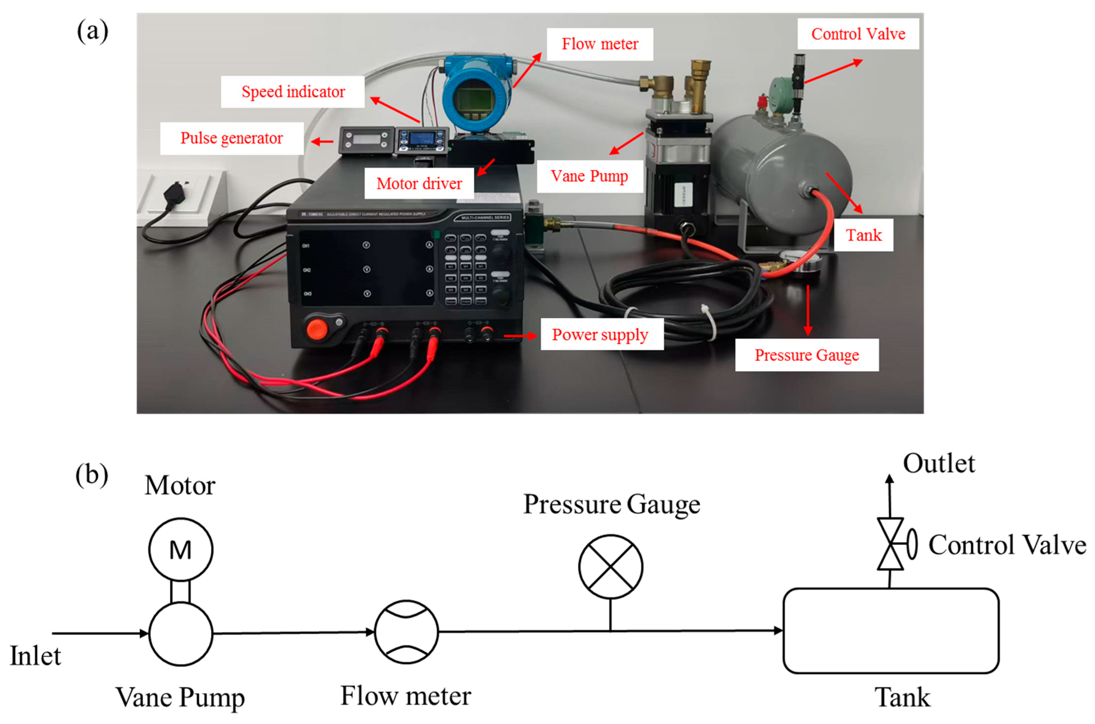
The experimental testing system for the vane pump is shown in Figure 5. The system consists of a flow meter (NND-TMF, Enaide, Dalian, China), a pulse generator (ZK-PP1K, Zhauto, Shenzhen, China), a speed indicator (KEDA-LED, FocusAi, Dongguan, China), a power supply (eTM-DM-III, eTOMMENS, Dongguan, China), a motor driver (WS3H15R, Zhauto, Shenzhen, China), the tested vane pump, a tank (YC-QW005B, Youcheng Zhixin, Suzhou, China), a pressure gauge (Y-60, Fangjun Instrument, Shanghai, China), and a control valve. The tested vane pump was manufactured according to the optimized geometric parameters obtained from the PSO-based multi-objective optimization. The flow meter is connected to the pump outlet to measure the exhaust flow rate. The discharge pressure is regulated by adjusting the valve opening at the tank outlet. As in the simulation, air was used as the working medium instead of gasoline vapor, a common and necessary simplification in pump performance testing due to the flammability and toxicity of real gasoline vapor. During the test, the rotational speed was set to 1500 r/min via the pulse generator, and the discharge pressure was adjusted to 103.825 kPa using the control valve. The exhaust flow rate was then read from the flow meter.

3. Results and Discussion

3.1. Optimization Results

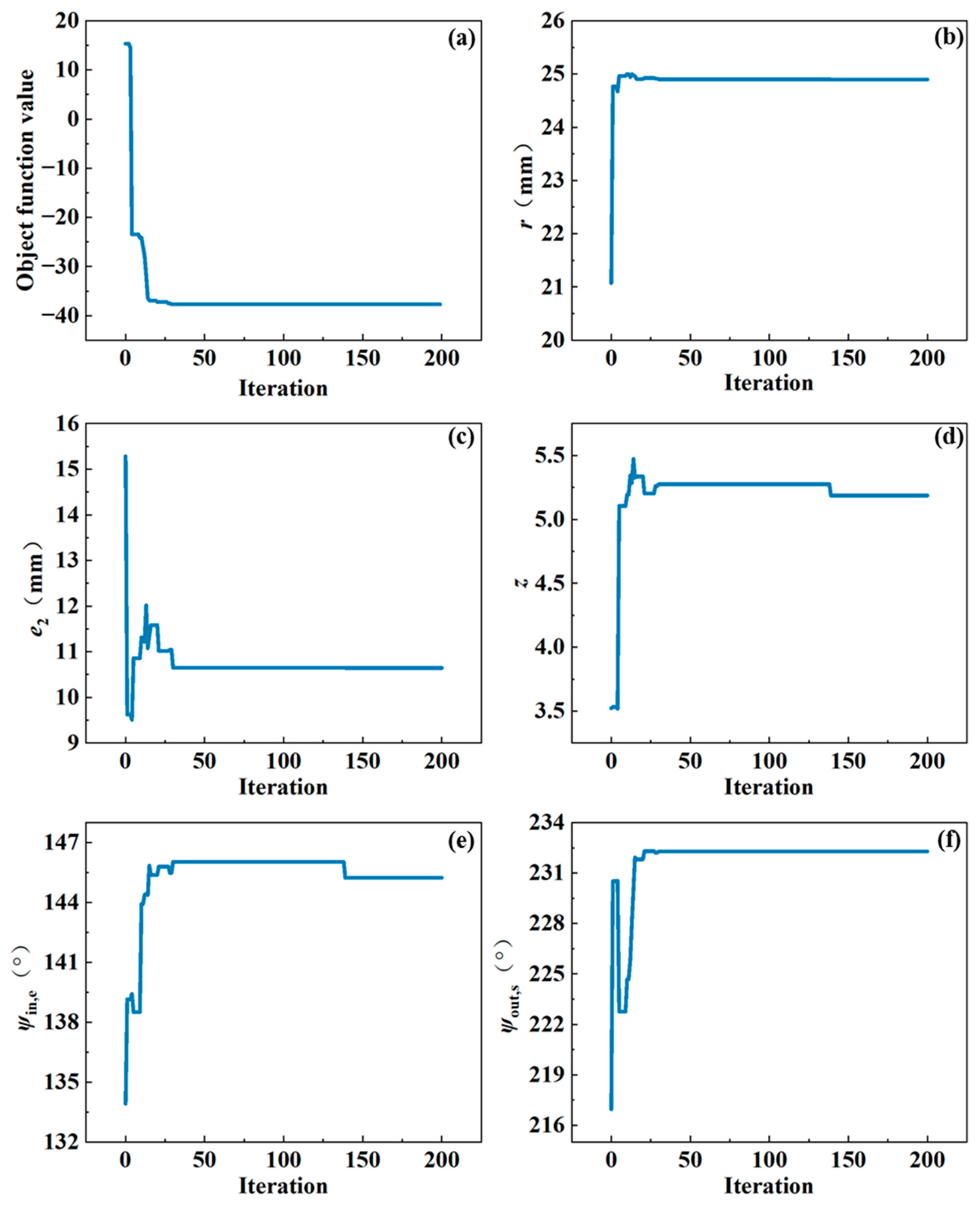
Figure 6 illustrates the convergence behavior of the PSO algorithm. The objective function value decreases rapidly and converges to approximately −37 by the 20th generation. The corresponding optimal performance metrics are Q_ave = 61.8 L/min and δ = 0.2426. The associated optimal design parameters are r = 24.9 mm, e₂ = 10.6 mm, z = 5, ψ_in,e = 145.2°, and ψ_out,s = 232.3°. Notably, the optimized pump delivers a 12.8% higher flow rate (61.8 L/min vs. 54.8 L/min) than the reference pump, even though its chamber radius is reduced from 33 mm to 30 mm.

During the initial iterations, pronounced fluctuations in the design variables suggest a global exploration phase across the solution space. As optimization progresses, the variables stabilize, indicating a transition to local refinement. All design variables converge within approximately the same number of iterations, indicating that the PSO parameters are well chosen for this problem. Furthermore, none of the final optimized values hit the predefined bounds, showing that the optimum is interior and not artificially constrained by the search limits.

The PSO results were validated through both simulation and experiment. The theoretical, simulated, and experimental flow rates are 61.8 L/min, 56.6 L/min, and 52.3 L/min, respectively. This decreasing trend can be attributed to the progressive relaxation of idealizations in the theoretical model and the incorporation of realistic losses in the numerical and experimental models.

The theoretical model adopts idealized assumptions of zero clearance between the rotor end faces and the end caps, and perfect contact between the vanes and the chamber wall, completely neglecting all internal leakages. The numerical model incorporates finite clearances of 3 × 10⁻⁵ m for the rotor end faces and 2.5 × 10⁻⁵ m for the vane tips. These clearances allow high-pressure gas to leak back to the suction side, causing volumetric losses that reduce the simulated flow rate below the theoretical prediction. The experimental value is even lower because the actual clearances in the manufactured pump are larger than the nominal design values due to machining tolerances and assembly errors. Thermal deformation and wear during operation further increase these clearances, resulting in more severe end-face and vane-tip leakages than those modelled numerically. This decreasing trend is physically consistent and reflects the progressive relaxation from an idealized leakage-free model to a design-clearance model and finally to a real manufactured prototype.

3.2. Correlation Analysis of Optimization Results

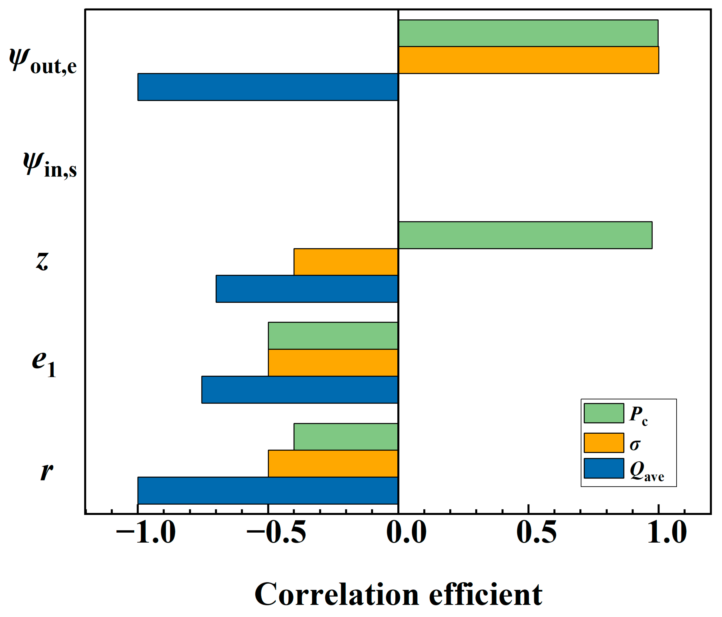
A correlation analysis was conducted to evaluate the influence of key geometric parameters on pump performance and to identify the dominant factors affecting the performance metrics. Each continuous variable was perturbed by ±5% from its optimal value (with the discrete vane number varied by ±2), while holding other parameters constant. The results of the correlation analysis between each optimization variable and the components of the objective function at the optimal point are presented in Figure 7.

The results show that at the optimal point, the correlation coefficient between ψ_out,s and P_c is −1, between ψ_out,s and δ is +1, and between ψ_out,s and Q_ave is +0.9977. The absolute values are all close to or equal to 1, indicating that changes in ψ_out,s exert a near-deterministic influence on all three quantities. Moreover, ψ_out,s is negatively correlated with P_c and positively correlated with δ; these opposite signs imply that increasing ψ_out,s reduces P_c while increasing δ, causing exhaust pressure and pulsation to change in opposite directions. The rotor radius r shows correlation coefficients of −1, −1, and −0.9818 with P_c, δ, and Q_ave, respectively, indicating strong negative correlations. Thus, increasing r reduces all three quantities simultaneously. While a lower r is beneficial for flow rate, it also increases pulsation and P_c, highlighting a trade-off that the multi-objective optimization must balance.

The number of vanes z exhibits a strong positive correlation with Q_ave (+0.9747) and weaker negative correlations with P_c (−0.7) and δ (−0.4). This suggests that increasing z raises the flow rate while moderately reducing pressure and pulsation. The eccentricity e₂ shows correlation coefficients of −0.7545, −0.5, and −0.5 with the three quantities, indicating a weaker influence than r and ψ_out,s. ψ_in,e shows a correlation coefficient of 0 with all objectives, indicating that near the optimal point, this parameter has no linear effect on Q_ave, P_c and δ.

3.3. Sensitivity Analysis of Constraints

A sensitivity analysis was conducted on two key constraints—λ and P_c—to systematically evaluate their influence on the optimal design variables. Sensitivity analysis examines whether the optimal design variables change significantly under constraint fluctuations, providing an indication of solution stability. Unlike global sensitivity analysis methods, which require extensive computational resources to quantify parameter interactions [33], the present study adopts a local percentage-change method that is well-suited for the deterministic theoretical model. The analysis employed the control variable method, taking λ and P_c as the constraint variables. Five levels were set for λ (0.55, 0.60, 0.65, 0.70, 0.75) and five for P_c (102.8, 103.3, 103.8, 104.3, 104.8 kPa) near the obtained optimal design point. For each constraint combination, other parameters were kept constant, and the optimization model was re-run to obtain the corresponding optimal design variable values. This generated a response dataset linking the constraint variables to the design variables.

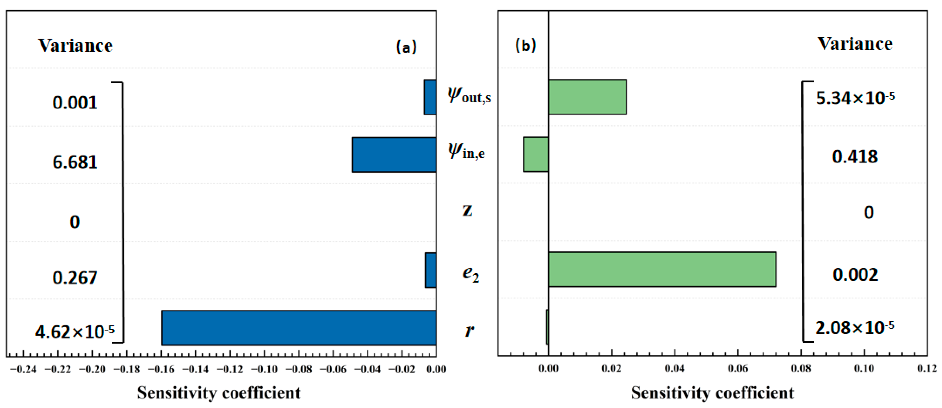
The sensitivity coefficient was calculated using the percentage change method. For each pair of adjacent levels, the ratio of the percentage change in the design variable to that in the constraint variable was taken as the sensitivity coefficient for that interval. The sensitivity coefficients from each interval were then averaged to obtain the overall sensitivity coefficient for each constraint–design variable pair, and the variance was also calculated. The constraint sensitivity coefficients and variances for the different optimization variables are shown in Figure 8.

The sensitivity analysis results show that the design variables respond differently to changes in the constraints. When λ increases, the optimal r decreases by 0.16 on average with a variance of only 0.0001, indicating an extremely stable response, which makes it the primary variable for matching the vane extension constraint. The ψ_in,e decreases by 0.049 on average but with a variance of 0.267, suggesting a clearly nonlinear response. e₂ shows an average response of only −0.006 but a variance as high as 6.68, indicating significant fluctuations when the vane extension length changes, which raises concerns regarding its stability. The response of ψ_out,s is weak and its variance is extremely small; thus, it can be considered negligible. The number of vanes z shows no response.

When the discharge pressure increases, the optimal e₂ increases by 0.072 on average with a variance of 0.418, indicating a noticeable response with some fluctuation. ψ_out,s increases by 0.025 on average with a variance of only 2.1 × 10⁻⁵, showing a stable and reliable response, which makes it the preferred variable for matching the discharge pressure constraint. ψ_in,e decreases by 0.008 on average with a small variance, indicating a stable but limited response. The response of r is extremely weak and can be considered negligible. The number of vanes still shows no response. In summary, sensitivity analysis shows that r is the primary tuning variable for the vane extension constraint, while ψ_out,s is the preferred variable for the discharge pressure constraint.

3.4. Mechanism of Exhaust Pulsation Improvement

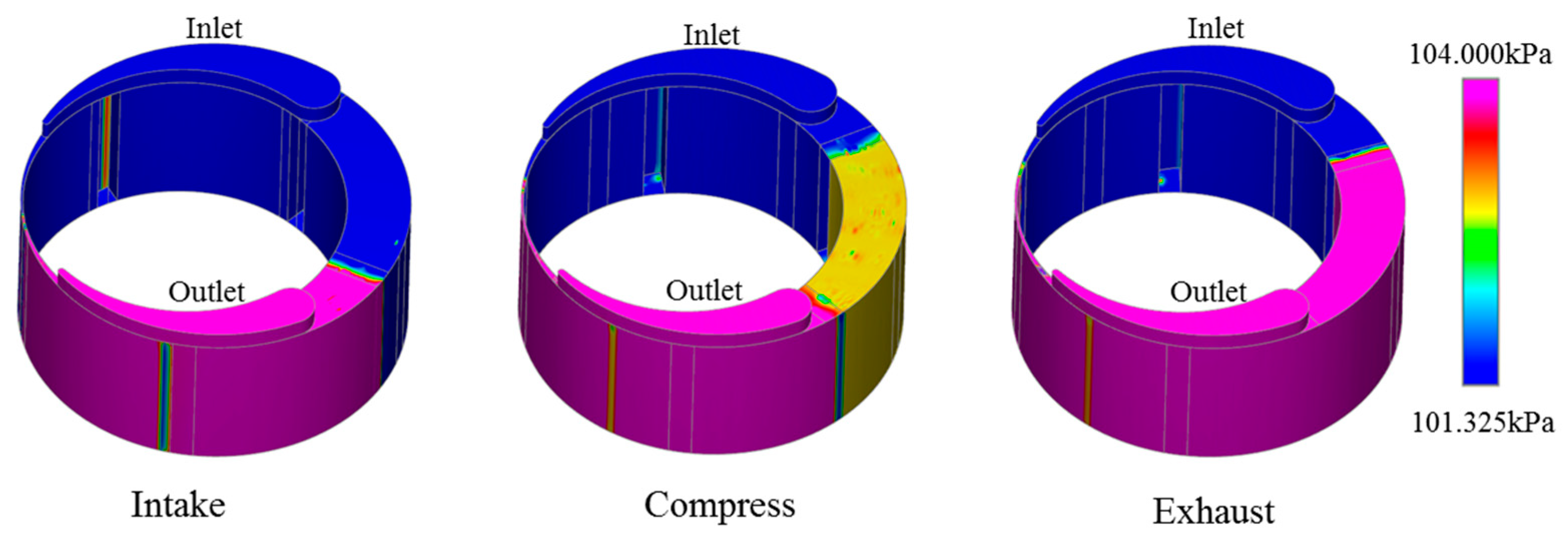
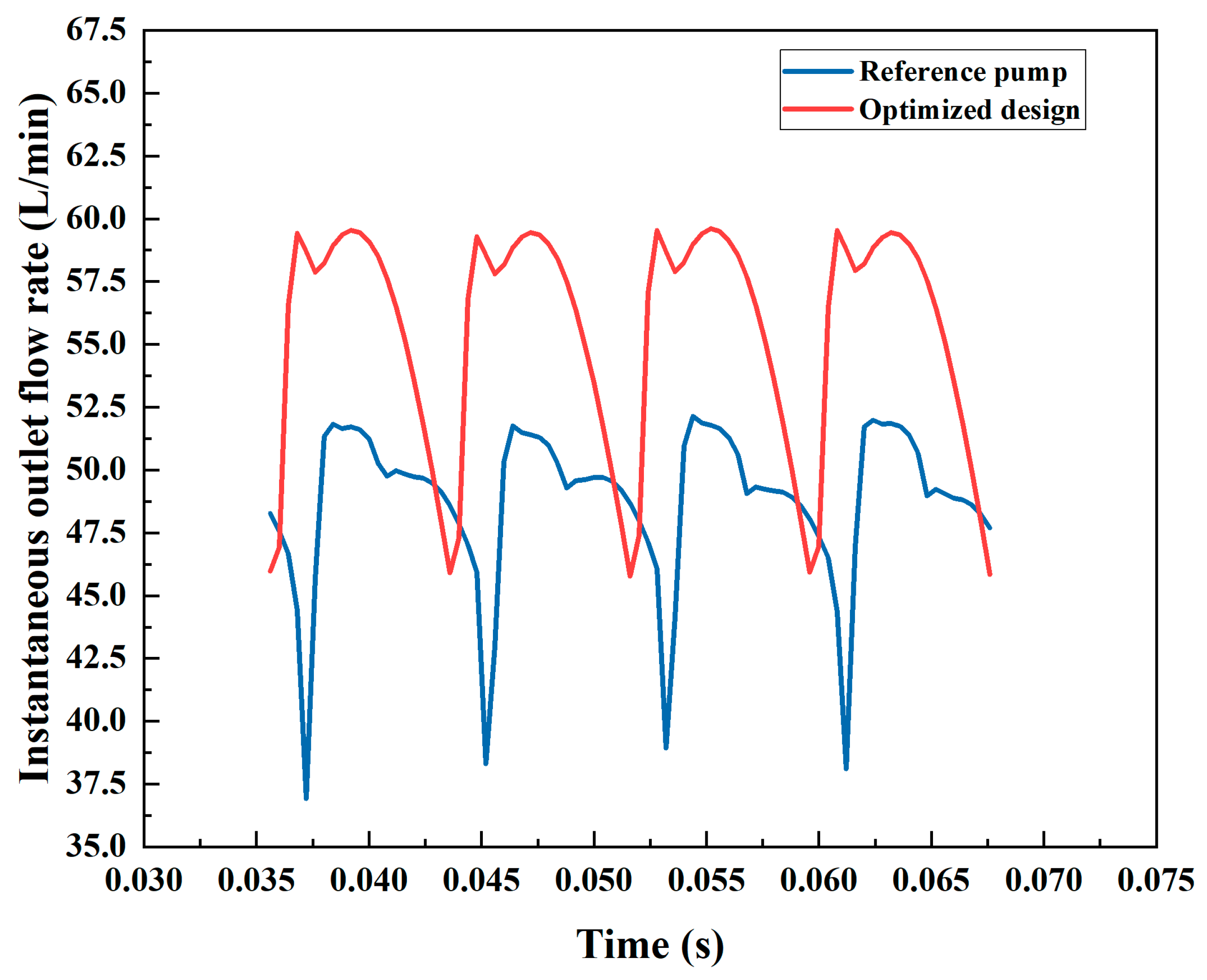
Figure 9 shows the pressure distribution within the pump. The pressure within a sealed chamber sequentially undergoes intake, compression, and exhaust, confirming that the numerical model captures the fundamental working cycle of the rotary vane pump. The improvement in δ is further reflected in the instantaneous flow rate curves. Figure 10 compares the instantaneous flow rate curves of the reference and the optimized pumps. After optimization, the average flow rate increased from 48.8 L/min to 56.6 L/min despite the chamber radius reducing from 33 mm to 30 mm. The underlying reason is that the rotor radius decreased from 29 mm to 24.9 mm through the optimization, which allows a larger vane eccentricity. The increased eccentricity enlarges the stroke volume of each working chamber, thereby raising the overall flow rate. Moreover, the peak-to-peak amplitude decreased from 15.2 L/min to 13.8 L/min, reflecting a notable reduction in flow fluctuation. δ decreased from 0.31 to 0.25, a reduction of 19.35%. Thus, the optimization successfully trades a smaller rotor for a larger eccentricity, resulting in a net gain in pumping capacity even under a more compact chamber size, and confirms that the optimized design significantly improves exhaust stability.

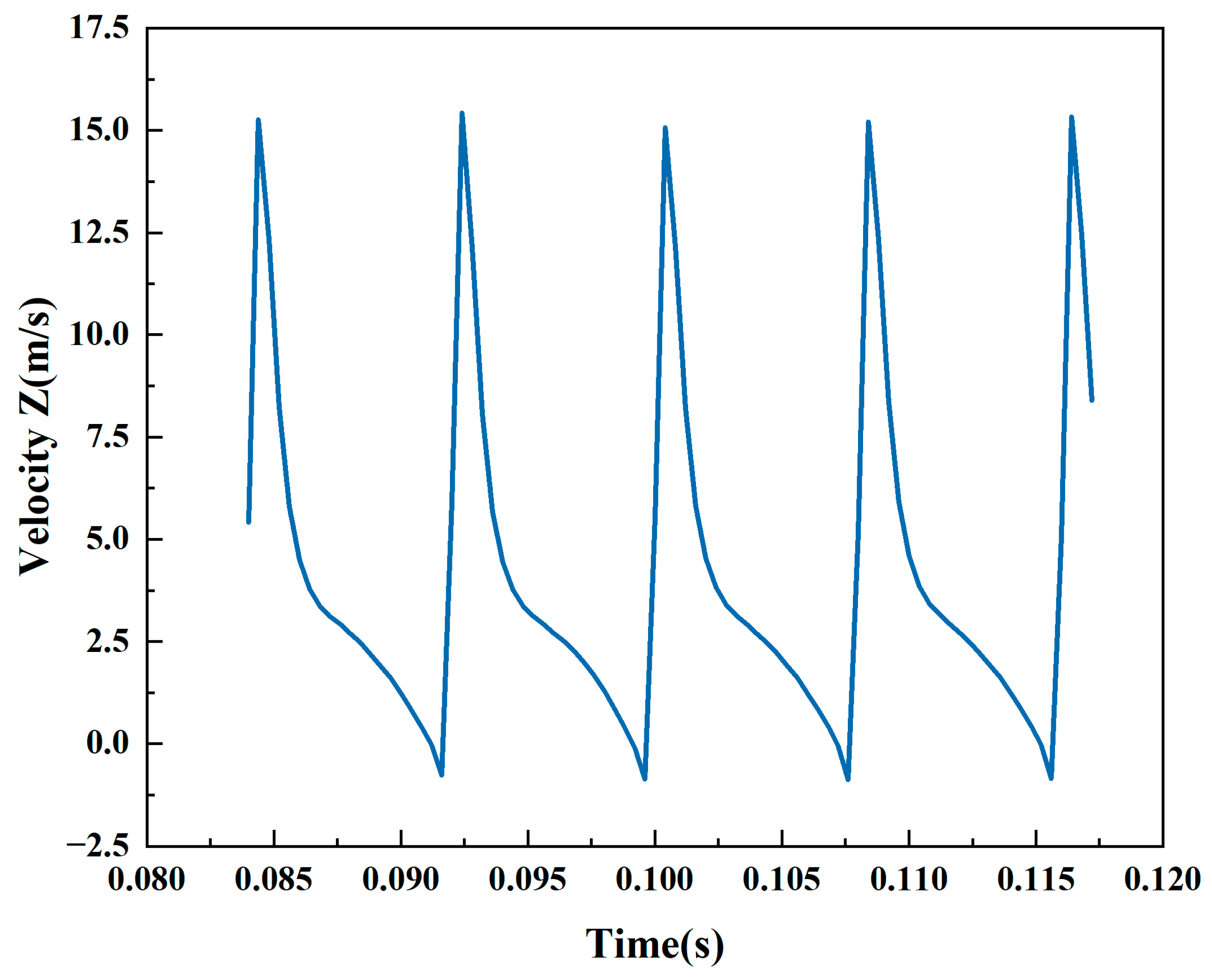
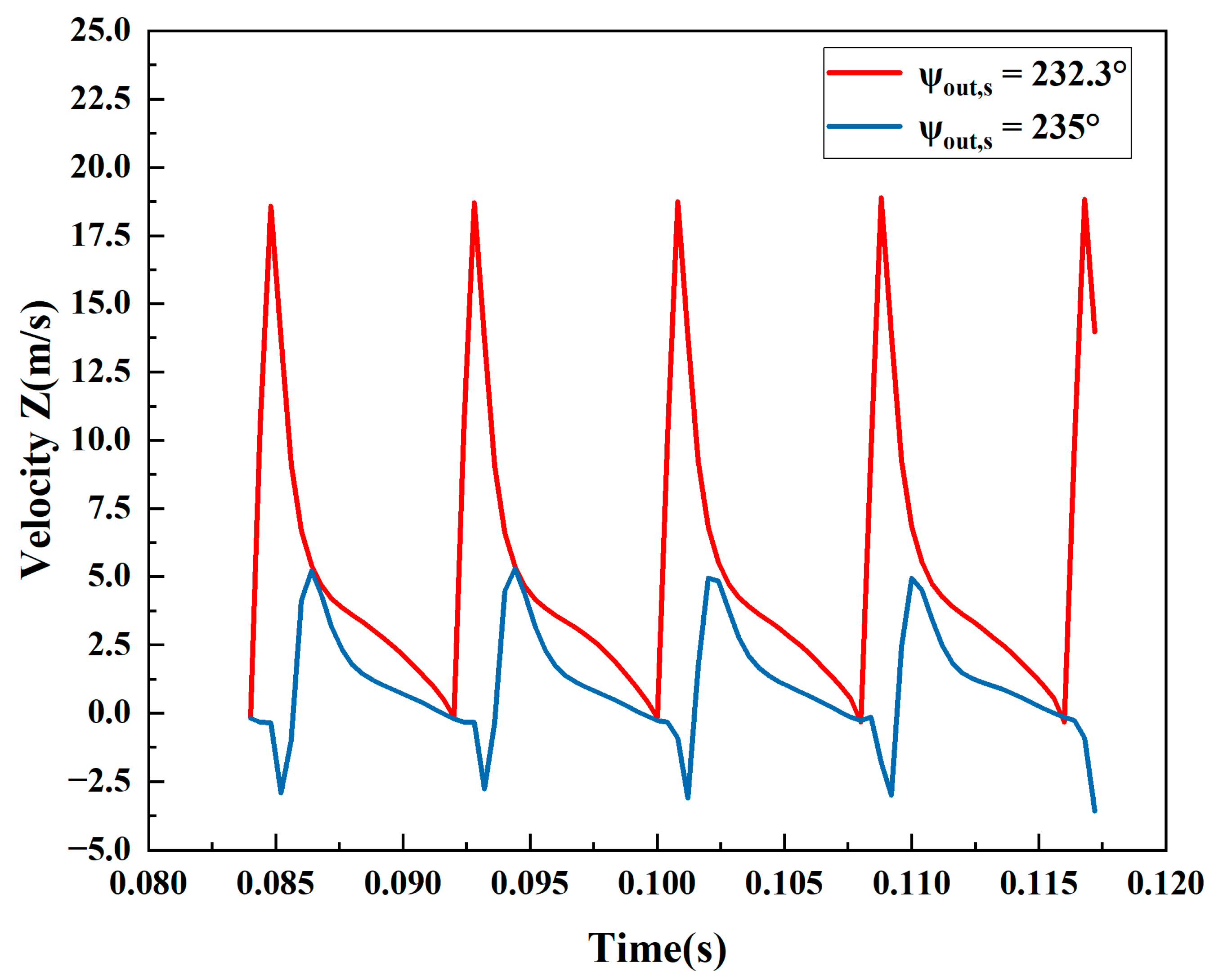
Although the optimized design reduces pulsation, backflow still exists. The reason is that the theoretical model’s prediction of pressure matching at ψ_out,s = 232.3° is not fully reproduced in the numerical simulation because of inherent model simplifications. Consequently, the chamber pressure at exhaust opening deviates slightly from the back pressure, causing residual backflow. Figure 11 presents the instantaneous velocity distribution at the exhaust port cross-section of the optimized pump. Negative velocities still appear, indicating that backflow persists. 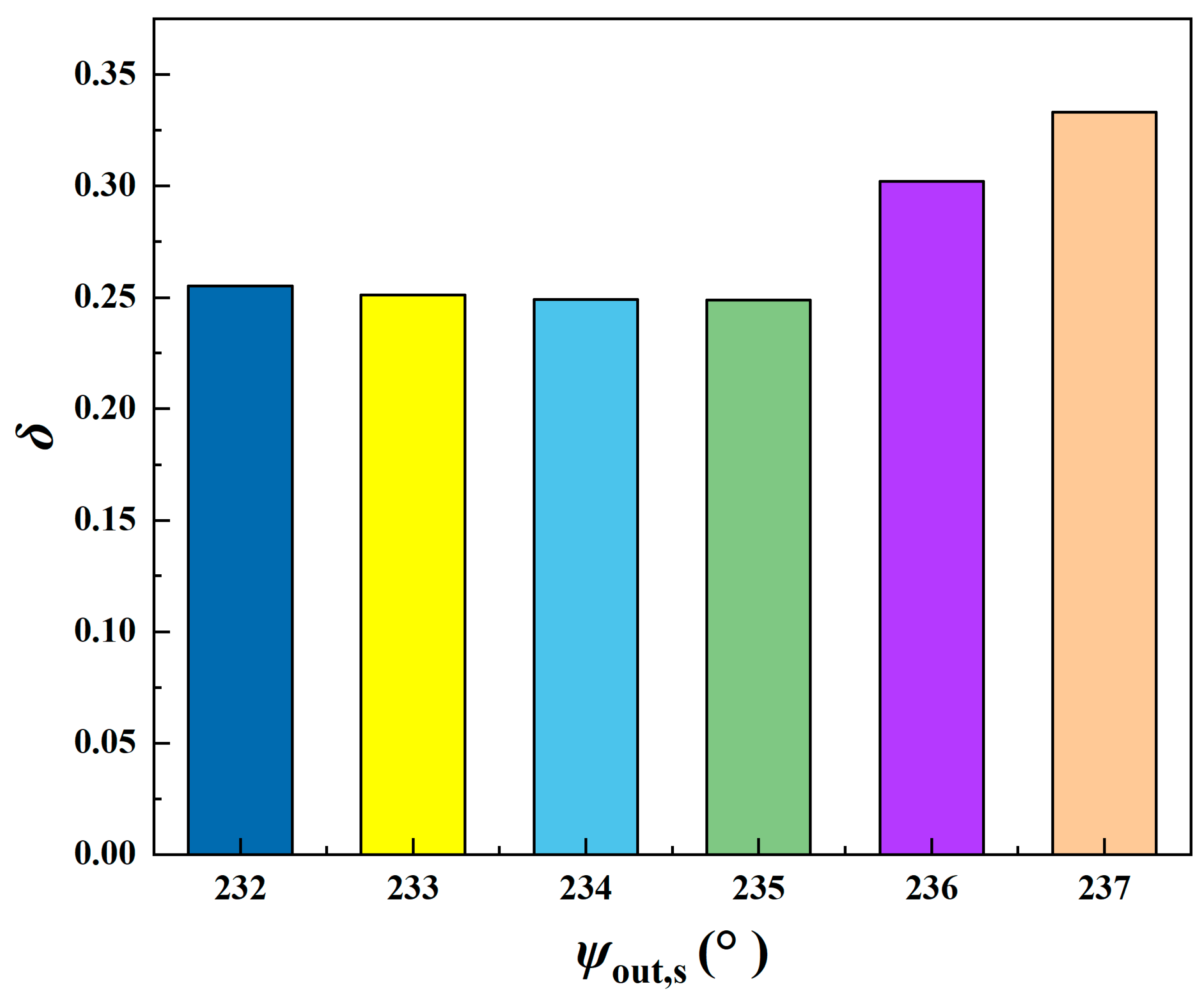Using the optimized ψ_out,s as a baseline, simulations were performed with varying exhaust port start angles to obtain the relation between this angle and δ, as shown in Figure 12. δ first decreases and then increases with ψ_out,s, reaching its minimum at 235°.

To reveal the mechanism of exhaust pulsation improvement, the internal flow field at the moment of exhaust port opening is analyzed. Figure 13 presents the velocity distribution at the exhaust port cross-section before and after the adjustment of ψ_out,s. Before adjustment (ψ_out,s = 232.3°), a large region of negative velocity is present, reaching as low as −3.58 m/s; after ψ_out,s is adjusted to 235°, the negative velocity region is significantly reduced, and the distribution becomes more uniform. 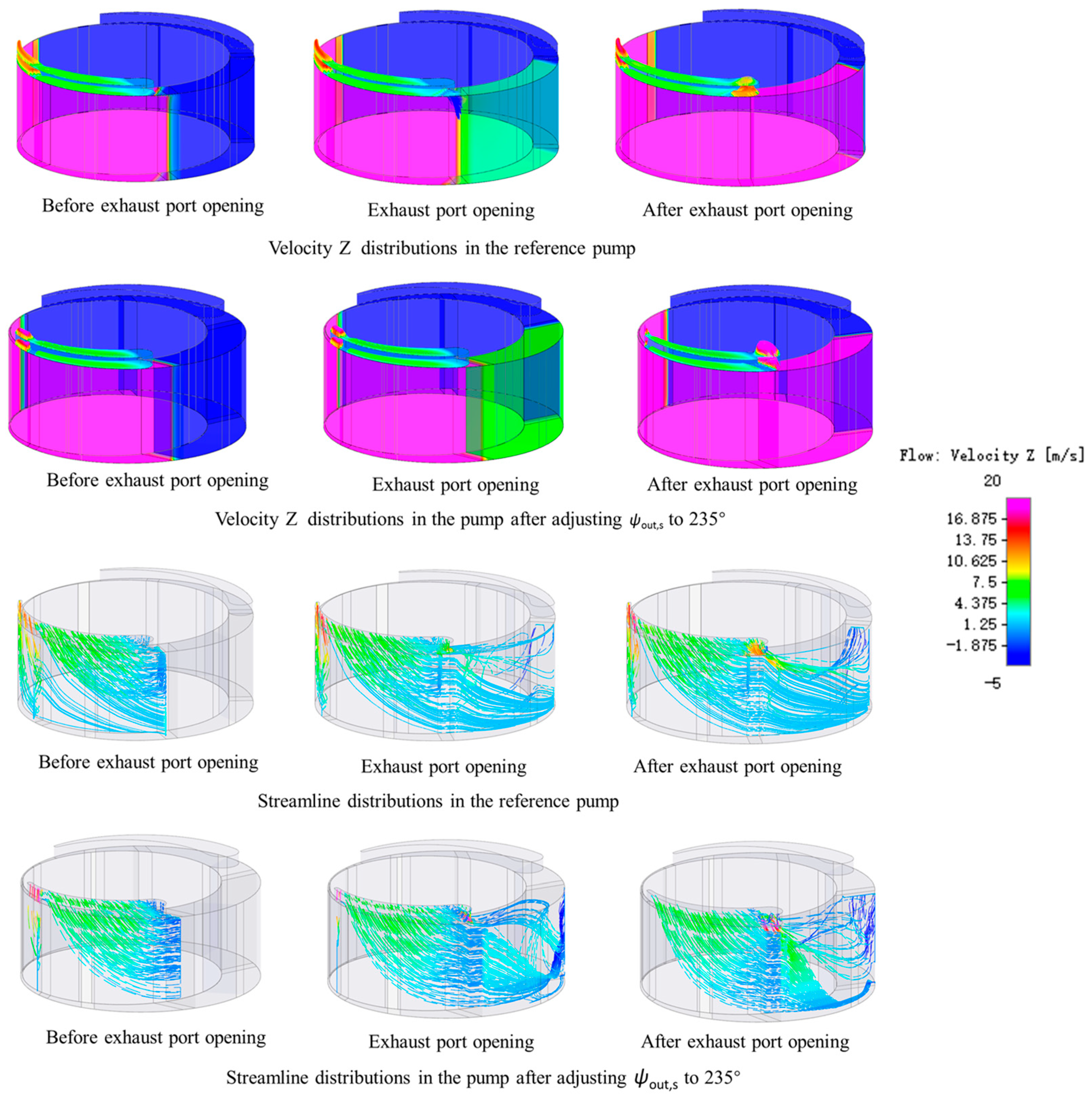Figure 14 compares the velocity Z and streamline distributions for the reference pump and after adjustment to 235°. For the reference pump, a negative velocity appears as the exhaust port opens, indicating backflow. After adjustment to 235°, this phenomenon is no longer observed.

Regarding the pump exhaust process, if ψ_out,s is too small, the exhaust opens too early, and the low chamber pressure leads to backflow. If ψ_out,s is too large, the exhaust opens too late, and the gas becomes over-compressed, resulting in a discharge shock. When ψ_out,s is at its optimal value, the gas in the closed chamber is compressed to a level much closer to the exhaust back pressure before the vane sweeps past the exhaust port. This avoids backflow or discharge shock caused by excessive pressure difference, achieving a good match between the chamber pressure and the exhaust back pressure. Backflow is effectively suppressed, over-compression is avoided, the exhaust process becomes smooth, and exhaust pulsation is minimized. Therefore, precise control of the exhaust port start angle is an effective way to achieve low-pulsation, high-stability exhaust design.

4. Conclusions

In this study, a multi-objective optimization using the PSO algorithm is performed to obtain the optimal design parameters for a rotary vane vapor recovery vacuum pump under fixed chamber radius and key constraints. The main findings are as follows.

(1)

Under a chamber radius of 30 mm, the optimal design parameters are r = 24.9 mm, e₂= 10.6 mm, z = 5, ψ_in,e = 145.2°, and ψ_out,s = 232.3°. The corresponding Q_ave = 61.8 L/min, representing a 12.8% increase over the reference pump with a chamber radius of 33 mm at 54.8 L/min, demonstrating improved performance with a more compact size.

(2)

At the optimal point, ψ_out,s exhibits the strongest local influence on performance, with correlation coefficients close to ±1; it is negatively correlated with discharge chamber pressure P_c and positively correlated with δ, indicating a clear trade-off. The rotor radius shows strong negative correlations with all objectives. A higher vane count increases Q_ave and tends to reduce both P_c and δ. ψ_in,e shows no linear effect and is therefore a redundant parameter near the optimum.

(3)

Constraint sensitivity analysis reveals that r responds stably to changes in λ, making it the primary adjustment variable for this constraint. Conversely, ψ_out,s responds stably to changes in P_c, serving as the preferred adjustment variable. e₂ exhibits notable fluctuations under both constraints, raising concerns about its stability.

(4)

Numerical simulations confirm that the optimized geometry achieves a well-matched exhaust process, characterized by a smooth pressure rise during compression and precise pressure-backpressure matching at exhaust initiation. The exhaust pulsation ratio δ first decreases and then increases with ψ_out,s, reaching a minimum at 235°, resulting in minimized δ and a smoother exhaust process.