Comparison of Rigid-Wall Computational Fluid Dynamics and Flexible-Wall Fluid-Structure Interaction in Descending Thoracic Aorta Aneurysm

Abstract

Currently, Computational Solid Mechanics (CSM) and Computational Fluid Dynamics (CFD) simulations are not enough to correctly estimate the different physical characteristics found in the human cardiovascular system. As an alternative to individual simulations, Fluid Structure Interaction (FSI) simulations can yield more accurate physical quantities. In this study a comparison between rigid-wall CFD of a thoracic aorta affected by an aneurysm and the FSI of the Descending Thoracic Aortic Aneurysm (DTAA) itself was performed. The 18-year-old patient-specific geometry of the aorta and its branches was based on the National Institutes of Health public database. A patient-specific pulsatile blood flow waveform and a pressure three-element Windkessel model were set for boundary conditions. Parameters such as wall pressure, velocity distribution, Wall Shear Stress (WSS), Time-averaged Wall Shear Stress (TAWSS), Oscillatory Shear Index (OSI), wall displacement and Von Mises Stress (VMS) were investigated. The research shown that blood flow in the aorta is strongly affected by the onset of the aneurysm, which causes recirculation and uneven flow within the aneurysmal bulge. The results highlight that rigid-wall CFD, which cannot capture wall deformation and aneurysm compliance, leads to an overestimation of velocity, WSS, and TAWSS by 15, 21, and $32\%$ respectively, compared to FSI during the systolic peak; furthermore, a key novelty is represented by the slight underestimation of pressure during the systolic peak, an aspect not previously detailed in the DTAA literature.

1. Introduction

The cardiovascular system exhibits highly complex fluid–structure interactions, where blood flow, pressure distributions, and wall shear stresses play central roles in both physiological function and the disease development [1,2,3]. Because many cardiovascular disorders (such as pulmonary hypertension, aneurysms, coronary artery diseases, etc.) are strongly influenced by local hemodynamic conditions, understanding the flow characteristics is essential for improving diagnosis, risk assessment, and treatment planning [4]. However, direct in vivo measurement of detailed flow fields remains challenging due to limitations in spatial resolution, invasive techniques, and inter-patient variability [5,6,7,8].

Computational Fluid Dynamics (CFD) has therefore emerged as a powerful tool for investigating cardiovascular hemodynamics with high fidelity [9]. By solving the governing equations of fluid motion within patient-specific domains, CFD enables researchers to explore local pressure gradients, velocity fields, and wall shear stress distributions that are otherwise difficult or impossible to measure experimentally [10,11,12]. Recent studies have demonstrated the value of CFD in analyzing pathological conditions, helping to quantify abnormal pressure loads and flow disturbances [9,13,14,15,16].

The integration of CFD with medical imaging and patient-specific modeling is transforming cardiovascular research. It allows clinicians and engineers to simulate disease scenarios, evaluate surgical interventions, and design personalized treatment strategies. As computational methods and imaging technologies continue to advance, CFD is becoming an indispensable component of modern cardiovascular biomechanics, offering a non-invasive, cost-effective, and highly detailed window into the dynamics of blood flow.

However, an accurate description of cardiovascular hemodynamics often requires not only modeling blood flow but also accounting for the mechanical response of vascular tissues, making Fluid-Structure Interaction (FSI) a fundamental component of advanced numerical simulations [17,18,19,20]. Blood vessels continuously deform under pulsatile pressure loads, and this deformation in turn alters the flow field, creating a bidirectional coupling that rigid-wall assumptions do not capture [11]. By integrating CFD with structural mechanics, FSI models offer a more realistic and physiologically accurate representation of the cardiovascular system, potentially enabling improved predictions of disease progression and offering more reliable support for medical evaluations.

Several numerical strategies have been developed to tackle the challenges FSI in hemodynamics [4]. The Arbitrary Lagrangian-Eulerian (ALE) framework [21,22] has become the most widely adopted approach due to its ability to accurately track the fluid-solid interface and its computational efficiency in partitioned solvers. However, it is well-known that ALE is primarily suited for small to moderate structural deformations (less than $10\%$) [23], as excessive displacements can lead to severe mesh distortion and to numerical instabilities.

In this context, more advanced numerical frameworks have recently emerged to overcome these limitations, especially for strongly coupled problems or extreme deformations. These include monolithic fully implicit formulations based on Eulerian representations of the elastic structure [24]. These approaches are particularly effective in handling strong coupling effects and avoiding the ’added mass’ numerical instabilities typical of partitioned schemes when dealing with lightweight structures in incompressible flows [25]. Despite these advancements, for the physiological range of the thoracic aortic wall displacements, which is the focus of the present study, the ALE framework remains a reliable and accurate choice [4,26,27].

In addition, there is also growing interest in the integration of machine learning (ML) and data assimilation techniques within the field of computational biomechanics [28]; however, high-fidelity CFD and FSI simulations remain indispensable tools, particularly for the study of descending thoracic aortic aneurysms (DTAA). To date, in fact, the literature concerning the application of ML models specific to DTAA is still limited compared to other vascular regions [29,30,31]. Direct numerical simulation is essential for generating the reference datasets required for the training and validation of future data-driven models [32,33], ensuring that they are physically consistent.

In various studies, FSI techniques have been adopted to investigate blood flow in different cardiovascular vessels, providing estimates of the main fluid-dynamic fields as well as the distribution of mechanical stresses within the vascular tissues [26,34,35,36]. Multiple studies demonstrate the clinical relevance of FSI simulations of aortic blood flow and aortic aneurysms, providing relevant parameters such as wall stresses, local wall deformations, pressure, velocities, while also enabling the visualization of the flow pattern in the aneurysm zone [37,38,39,40,41,42]. In addition, FSI and finite element-based computational techniques are essential for the analysis of native and pathological valve haemodynamics, as well as for the design and optimization of implantable heart valves [43,44]. Recent studies have investigated the fluid–structure interaction of healthy aortic valves and the surrounding flow field [45], the influence of bicuspid aortic valve cusp fusion patterns on aortic wall shear stress distributions [46], and patient-specific computational haemodynamics for pulmonary valve replacement [47]. These works demonstrate the relevance of numerical modeling for quantifying wall shear stress and related haemodynamic indicators in valvular flows. With respect to these contributions, the present study focuses on a comparison between classical CFD and FSI simulations for blood-flow in cardiovascular system.

In the last year, only a few studies have focused on comparing fully coupled fluid–structure interaction (FSI) of Descending Thoracic Aortic Aneurysm (DTAA) models with rigid-wall CFD and other simplified approaches for patient-specific aortic simulations [37,48,49,50,51,52]. These investigations consistently demonstrate that while rigid models can approximate global metrics, such as pressure and flow waveforms, they fail to capture compliance-driven local phenomena [53], including wall shear stress and secondary flow patterns, which are critical for accurate risk assessment [54,55].

In this context, this work aims to contribute to this topic by comparing rigid-wall CFD and flexible-wall FSI simulations of blood flow in a patient-specific descending thoracic aortic aneurysm, highlighting the capability of FSI simulation to capture wall compliance and the role of the aneurysmal sac as a flow accumulation zone. We selected a case study of a patient-specific aortic geometry, with pulsatile blood flow waveforms. For the pressure outlet boundary conditions, we rely on a three-element Windkessel model [56].

2. Materials and Methods

2.1. Geometry

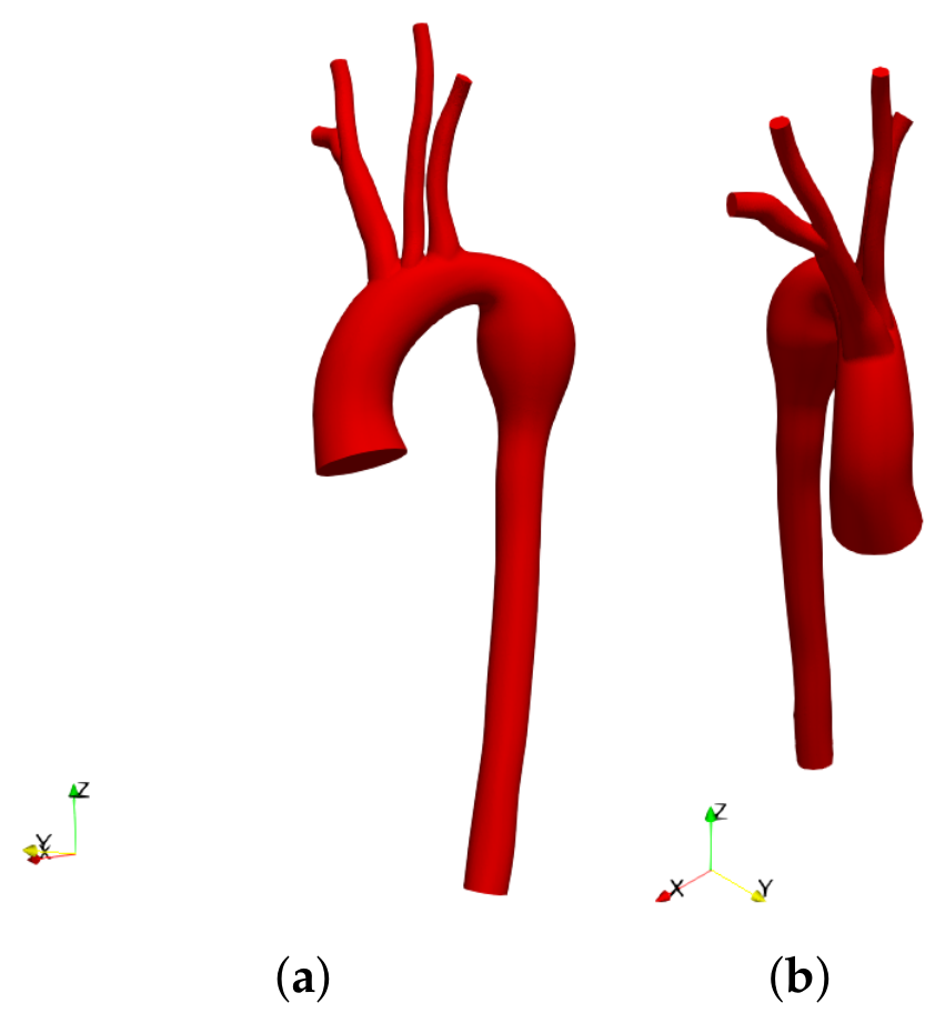
For this study, a publicly available three-dimensional model of the thoracic aorta was obtained from the National Institutes of Health (NIH) database [57], ensuring reproducibility and accessibility. The model, shown in the Figure 1, represents an 18-year-old patient with a descending thoracic aortic aneurysm. The domain for the FSI simulation is the downstream part of that in the CFD simulation, more precisely from “Cut for FSI” to Outlet in Figure 2a.

2.2. CFD Set-Up

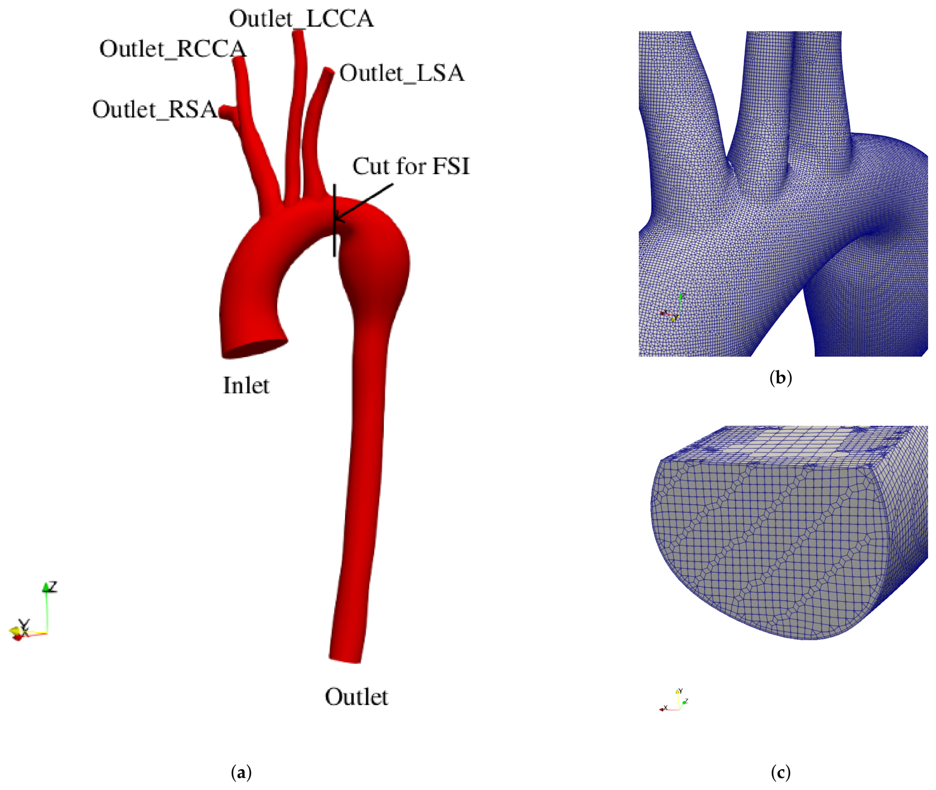
To ensure consistency between the rigid-wall CFD and flexible-wall FSI analyses, an initial CFD simulation was conducted on the full aortic geometry. The resulting flow data were mapped onto a newly defined inlet section (Cut for FSI), which was used as the inlet boundary condition for the FSI simulation, as depicted in Figure 2a.

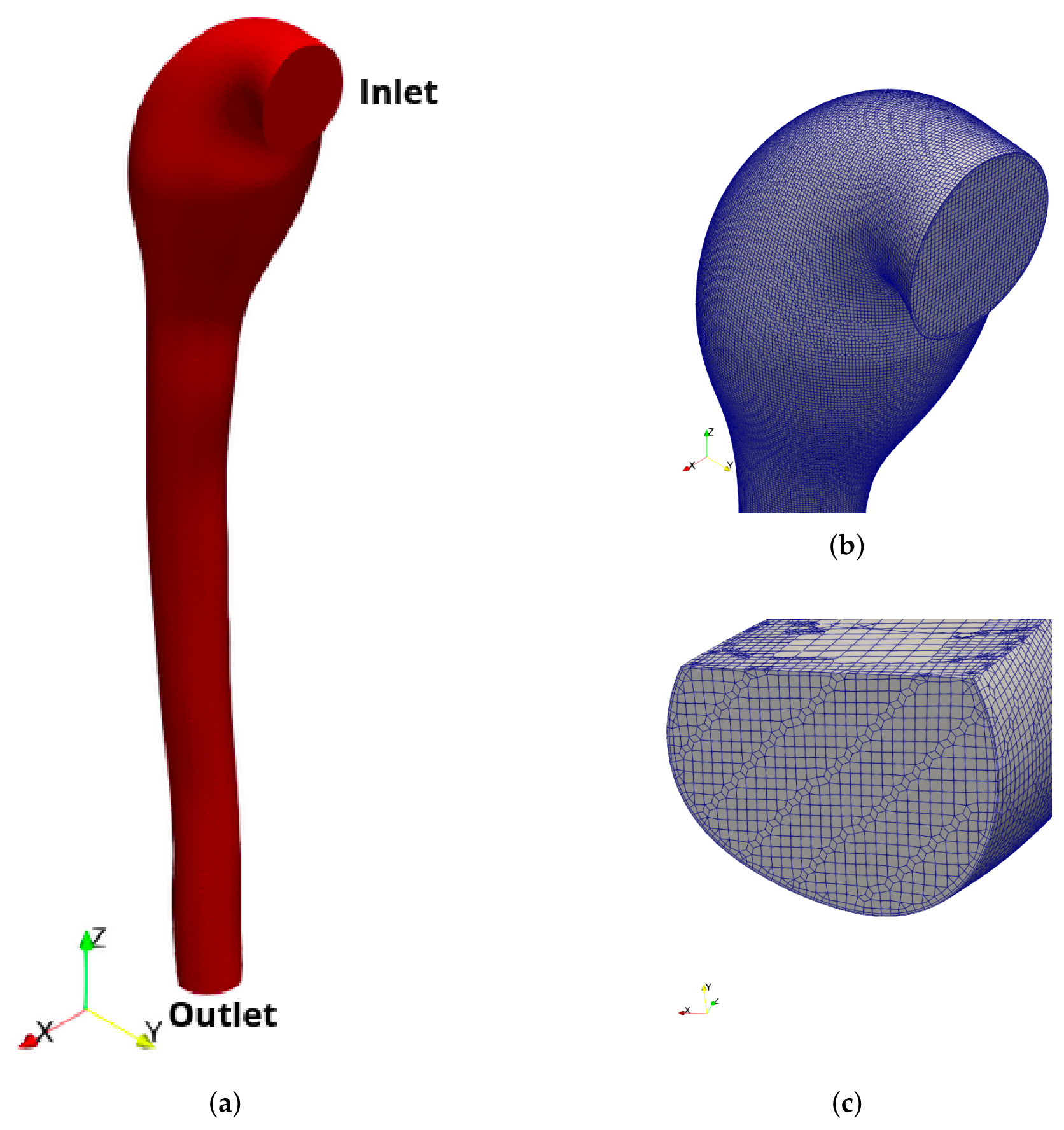
The mesh was built with cfMesh [58] and consisted of 861201 cells, and it is shown in Figure 2b,c. The adopted computational mesh was determined through a systematic grid sensitivity analysis, described in detail in the Section 2.2.3, employing the Grid Convergence Index (GCI) method, ensuring mesh-independent numerical results [59].

2.2.1. CFD Numerical Simulation

The fluid problem was modeled using the Navier-Stokes equations, considering an incompressible, laminar fluid. Blood, as is well known, is a non-Newtonian and shear-thinning fluid [60] due to its complex composition and the interactions between its components. In particular, when the shear rate exceeds 100 s⁻¹ [1,13] and in the case of large vessel diameters relative to red blood cell size, it is commonly accepted in the literature to consider blood as a Newtonian fluid [4,14,61,62]. It should be noted, however, that in areas of low shear rate, such as the aneurysmal sac Newtonian models can lead to variations in haemodynamic parameters such as WSS [41,63,64]. In this particular study, the focus is on the aorta where the diameters are larger than 0.1 mm, allowing blood to be treated as a Newtonian fluid

$$\begin{array}{cc}\hfill {\rho }_f\left[{\displaystyle \frac{\partial {\mathbf{u}}_f}{\partial t}}+({\mathbf{u}}_f·\nabla ){\mathbf{u}}_f\right]+\nabla p-\mu \Delta {\mathbf{u}}_f& =0\hfill \end{array}$$

(1)

$$\begin{array}{cc}\hfill \nabla ·{\mathbf{u}}_f& =0\hfill \end{array}$$

(2)

where ${\mathbf{u}}_f$ is the fluid velocity field, p is the pressure and ${\mu }_f$ is the dynamic viscosity.

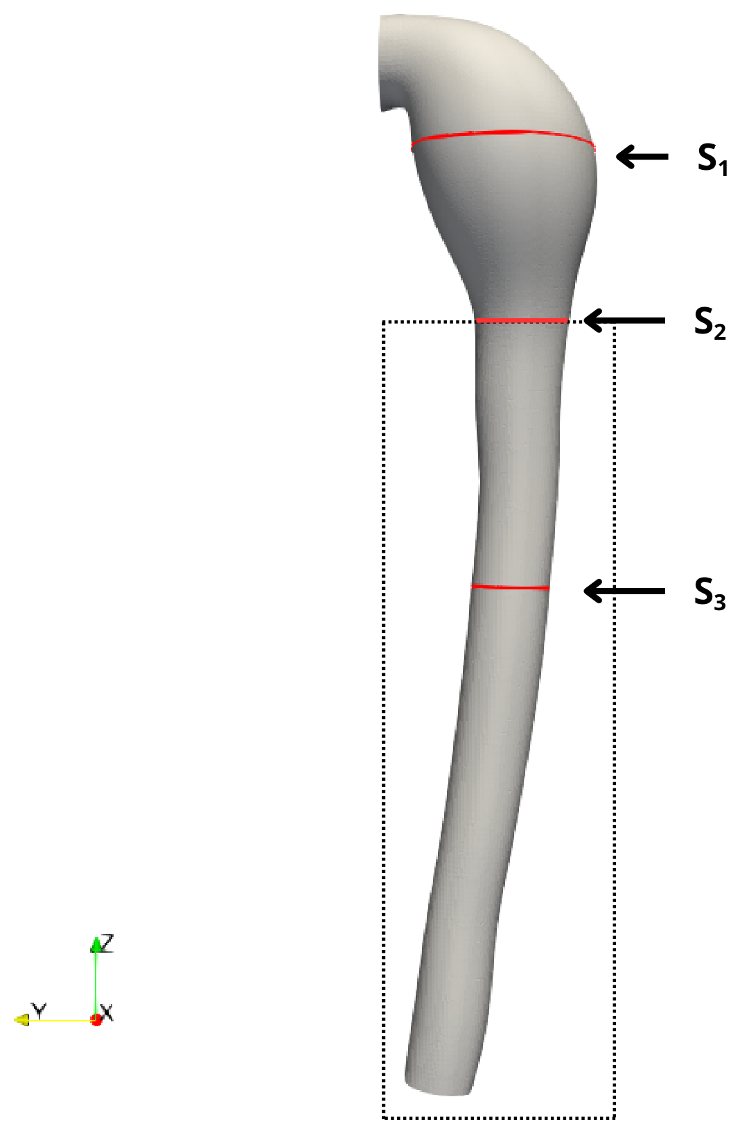
Considering the sections with the largest diameter and peak velocity, $S_1$ and $S_3$, depicted in Figure 3, the Reynolds number ($Re$) calculated during the systolic peak is found to be 1833 and 4072 respectively. Although the value of the $S_3$ section is in the transition regime, the laminar flow model is still valid. Indeed, considering the critical Reynolds model ($R{e}_c$) in the thoracic aorta [65,66]

$$R{e}_c=k\alpha$$

(3)

where k is a constant between 250 and 1000 and $\alpha$ is the Womersley number which is equal to $21.9$ for section $S_1$ and 10 for section $S_3$. The resulting range of values, respectively for $S_1$ and $S_3$, is 5475 to 21,900 and 2500 to 10,000, which is higher than the calculated Re numbers. Furthermore, the calculated Re values are the maximum values found in the critical section of our domain and occur only during small part of the cardiac cycle.

The blood was modeled with a density of 1060 kg/m³ and a kinematic viscosity [9,67] of $4\times {10}^{-6}$ m²/s. Implicit first-order Euler method was used for temporal discretisation to ensure high numerical stability, which is critical in FSI problems with a high ratio of added mass to structural mass, such as this one. A variable time step of the order of $1\times {10}^{-3}$ s was chosen. In terms of spatial discretisation, second-order schemes were chosen; specifically, the Gauss-linear scheme for the gradient, the Gauss-linear-Upwind scheme for the divergence, and the Gauss-linear-corrected scheme for the Laplacian term. The PIMPLE algorithm was adopted to compute the solution, with the end of the cycle controlled by tolerances on velocity and pressure residuals of $1\times {10}^{-8}$ and $1\times {10}^{-7}$, respectively.

2.2.2. Boundary Conditions

A three-element Windkessel model was used to model the pressure boundary condition for the RSA, RCCA, LCCA, and LSA outlets. They represent the Right Subclavian Artery, the Right Common Carotid Artery, the Left Common Carotid Artery, and the Left Subclavian Artery. The following equation describes the Windkessel model:

$${\displaystyle \frac{dP\left(t\right)}{dt}}={\displaystyle \frac{(Z+R)}{CR}}Q\left(t\right)+Z{\displaystyle \frac{dQ\left(t\right)}{dt}}-{\displaystyle \frac{P\left(t\right)}{CR}}$$

(4)

where Q is the flux and the R, Z and C parameters are specific to each patient and are related to mean aortic pressure and flow rate [56,68]; their values are reported in

Table 1. Resistance and compliance values used.

	R $\left[\frac{\mathbf{Pa} \times \mathbf{s}}{{\mathbf{m}}^3}\right]$	Z $\left[\frac{\mathbf{Pa} \times \mathbf{s}}{{\mathbf{m}}^3}\right]$	C $\left[\frac{{\mathbf{m}}^3}{\mathbf{Pa}}\right]$
LCCA	$2.18\times {10}^8$	$6.58\times {10}^8$	$2.42\times {10}^{-9}$
LSA	$1.74\times {10}^8$	$5.24\times {10}^8$	$3.04\times {10}^{-9}$
RCCA	$1.71\times {10}^8$	$5.14\times {10}^8$	$3.09\times {10}^{-9}$
RSA	$1.32\times {10}^8$	$3.98\times {10}^8$	$4.00\times {10}^{-9}$

and can be defined from patient-specific haemodynamic measurements, mainly cardiac output and mean aortic pressure, as reported in the literature [56,68,69,70]. In particular, the total vascular resistance is distributed between $R_p$ and $R_d$, with $R_p$ set to 10% and $R_d$ to 90% of the overall resistance, following previous studies [13,69]. The three-component Windkessel model provides an accurate description of the role of aneurysmal compliance and vascular resistance. In particular, the capacitive element accurately simulates arterial dilation during systole, where energy is stored and subsequently released during diastole when the heart relaxes, thereby maintaining proper blood flow and pressure. The resistive elements, on the other hand, allow for the simulation of the resistance encountered by the blood flow as it moves in small and large vessel. The above boundary condition was implemented as a Dirichlet condition for pressure in the OpenFOAM software, version 2012 [71]. The ordinary differential equation (ODE), expressed by Equation (4), was solved using backward discretization method.

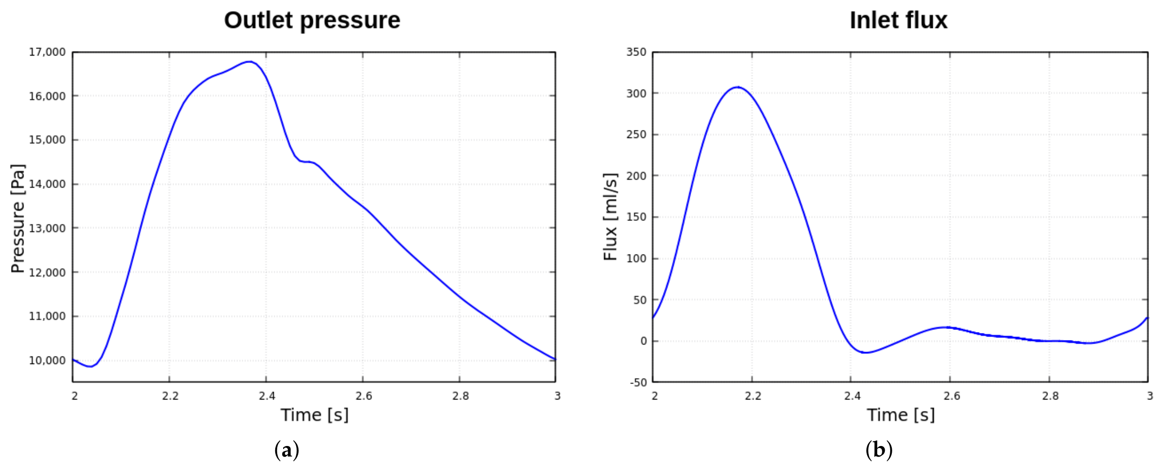
A pulsatile pressure waveform [72] was prescribed as a Dirichlet boundary condition at the descending aortic outlet, referred to as Outlet, as illustrated in Figure 4a. The volumetric flow rate, Figure 4b, was imposed at the Inlet as the boundary condition.

2.2.3. Mesh Sensitivity Analysis

Three grids, M1, M2 and M3, ranging from the finest to the coarsest (

Table 2. Mesh characteristics, where $h_{average}$ refers to average size of edge length.

Mesh	n° Cells	WSS $\left[\mathbf{Pa}\right]$	Flow Rate $\left[\frac{\mathbf{mL}}{\mathbf{s}}\right]$	${\mathbf{h}}_{\mathbf{average}}\left[\mathbf{mm}\right]$
M1	2,949,145	$6.861$	$208.806$	$0.359$
M2	861,201	6.844	$208.880$	$0.542$
M3	289,731	$6.739$	$208.909$	$0.779$

) were analyzed to assess mesh sensitivity. The GCI was evaluated for the WSS in the region highlighted by the box in Figure 3, corresponding to the DTA section downstream of the aneurysm at peak systole. In addition, the GCI for the volumetric flow rate was computed at section $S_3$ in Figure 3. To ensure an appropriate calculation of WSS, the flow near the wall needs to be properly captured through a y+ value that should be less than 2 [41,42,73]. In our case, a posterior check shows that for mesh $M_2$, which has a first layer thickness of $0.05$ mm, the y+ value is less than 2 during the systolic peak, which is the most critical point for this parameter due to the highest velocities. The section chosen is part of the FSI simulation domain where, due to wall deformation (which we will discuss later), lower velocities are observed; this results in lower $y^{+}$ values, which ensure an even more accurate WSS calculation, given the consistency of the fluid mesh used in both models. For the reasons explained earlier and due to high computational cost of FSI simulation, it was decided to carry out the sensitivity analysis exclusively for the CFD simulation.

The results of the grid sensitivity analysis are shown in

Table 3. Grid Convergence Index and the order of convergence for the WSS and Flow rate.

Mesh	${\mathbf{GCI}}_{\mathbf{wss}}$	${\mathbf{GCI}}_{\mathbf{Flow}\mathbf{rate}}$	Refinement Factor $\mathbf{r}=\frac{{\mathbf{h}}_{\mathbf{coarse}}}{{\mathbf{h}}_{\mathbf{fine}}}$
M1–M2	$0.040\%$	$0.021\%$	1.51
M2–M3	$0.331\%$	$0.010\%$	1.44

. As shown, the GCI values associated with the medium mesh are below $0.04\%$ for WSS and $0.02\%$ for flow rate when compared with the finest mesh, indicating negligible discretization errors. Consequently, the medium mesh (M2) was deemed sufficiently accurate and was adopted for all subsequent simulations.

2.3. FSI Set-Up

The FSI simulation was performed only on the portion of the thoracic aorta affected by the aneurysm. For the fluid domain, the geometry and mesh shown in the Figure 5 were used.

The framework used consists of OpenFOAM [71], CoCoNuT [74], and Abaqus [75]. The first solver was used for the fluid-dynamic problem, while the last was used for the structural one; CoCoNuT, serves as the coupling interface between the fluid and structural solvers.

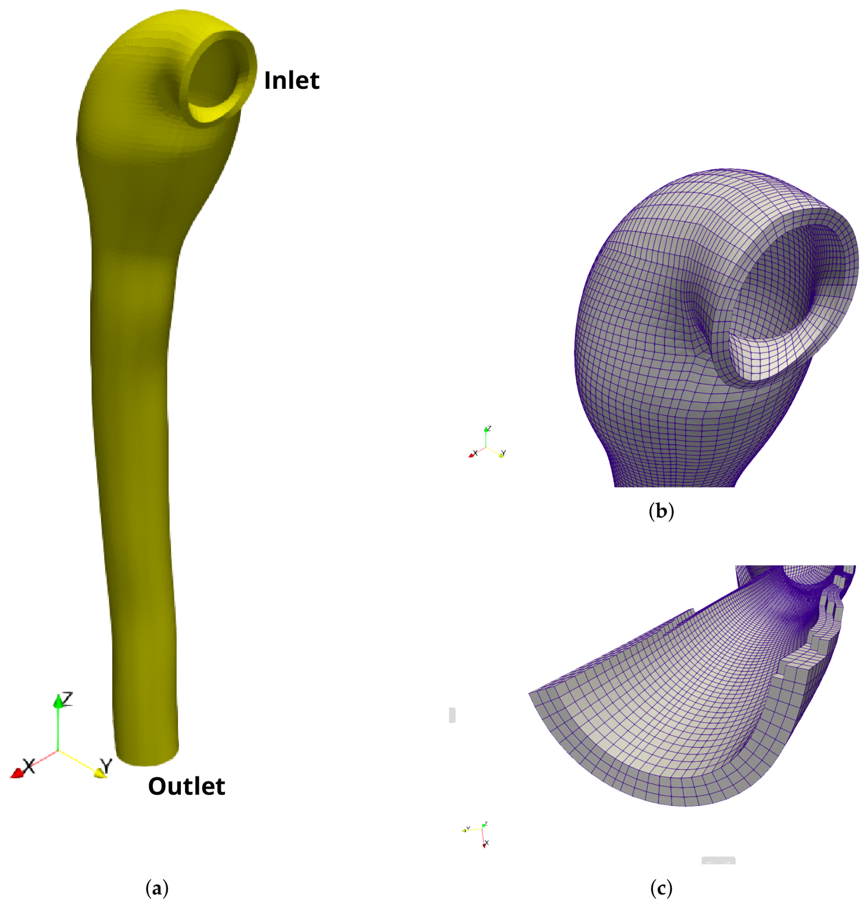
The CFD simulation results were used to extract the velocity values at the Cut for FSI cross section, which were then mapped and used as inlet boundary condition for the FSI simulation. In the FSI case, the fluid domain mesh consists of 447,623 cells and is depicted in Figure 5b,c.

The mesh for the aortic walls, shown in Figure 6, was generated by extruding the surface defining the fluid domain in the normal direction. The wall thickness is uniform and equal to 2 mm [11,76], discretized into 3 layers of hexahedral cells. This number of layers was chosen to ensure accuracy and acceptable computational time for the FSI simulation, as described in [26]. The solid domain mesh consists of 34,632 hexahedral cells and was created using ICEM software, version 2024 R1.

2.3.1. FSI Numerical Simulation

The FSI calculation consists of a fluid domain ${\mathsf{\Omega }}_f$ and a solid domain ${\mathsf{\Omega }}_s$. The fluid domain was modeled using the same equations and method described in the Section 2.2.1. The aortic wall consists of the intima, media and adventitia, separated by an elastic membrane [77]. The intima is the thinnest inner layer of the three, the media is the middle layer, and the adventitia is the outer, elastic layer. Such a complex tissue would require, as a constitutive model, the use of anisotropic models such as the Holzapfel-Gasser-Ogden (HGO) model [78,79]. However, most of the literature uses linear and non-linear isotropic models [4,37,41,76], despite recognising their limitations in terms, for example, of stress and strain evaluation [80]. In this study, the solid domain was modelled using a Neo-Hookean hyperelastic model [81], cf. Equation (5), with a Poisson’s ratio of $0.45$, a value close to incompressibility, a Young’s modulus of $1$ MPa and a density of $1000{\displaystyle \frac{\mathrm{kg}}{{\mathrm{m}}^3}}$. The material model is based on the following equation

$$\varphi (\mathit{B},J)={\displaystyle \frac{\mu }{2}}\left[J^{-{\displaystyle \frac{2}{3}}}tr\left(\mathit{B}\right)-3\right]+{\displaystyle \frac{\kappa }{2}}\left[{\displaystyle \frac{1}{2}}(J^2-1)-lnJ\right]$$

(5)

where $\varphi$ is the strain energy density function, $\mathit{B}$ is the Cauchy-Green deformation tensor, J is the Jacobian determinant of the deformation gradient, $\mu$ is the second Lamé parameter and $\kappa$ is the bulk modulus. As mentioned earlier, in the absence of patient-specific clinical data non-linear isotropic material, even though the effects of anisotropy and the multilayered nature of the aortic wall are neglected, provides a reasonable compromise between model complexity and computational cost, allowing the investigation of main haemodynamic parameters and wall deformations [4,26,42,82].

The motion of the solid domain is governed by the balance of linear momentum:

$${\rho }_s{\displaystyle \frac{{\partial }^2{\mathbf{d}}_s}{\partial t^2}}=\nabla ·{\mathit{\sigma }}_s+{\rho }_s{\mathbf{b}}_s\mathrm{in}{\mathsf{\Omega }}_s,$$

(6)

where ${\rho }_s$ is the solid density, ${\mathbf{d}}_s$ is the displacement field, ${\mathit{\sigma }}_s$ is the Cauchy stress tensor of the solid, and ${\mathbf{b}}_s$ is the body force per unit mass. The solid stress tensor ${\mathit{\sigma }}_s$ is obtained from the Neo-Hookean strain-energy density function reported in Equation (5).

FSI simulations require that two equilibrium conditions [36] be satisfied at the fluid-structure interface ${\Gamma }_{\mathrm{FSI}}$. The first is the kinematic condition:

$${\mathbf{u}}_f={\displaystyle \frac{d{\mathbf{d}}_s}{dt}}\mathrm{on}{\Gamma }_{\mathrm{FSI}}$$

(7)

where ${\mathbf{d}}_{\mathbf{s}}$ is the displacement vector of the solid domain at fluid–structure interface, and ${\mathbf{u}}_{\mathbf{f}}$ is the fluid velocity evaluated on the fluid side of the interface.

The second condition is the dynamic equilibrium at the interface:

$${\mathit{\sigma }}_f·{\mathbf{n}}_f=-{\mathit{\sigma }}_s·{\mathbf{n}}_s\mathrm{on}{\Gamma }_{\mathrm{FSI}}$$

(8)

where ${\mathit{\sigma }}_f$ and ${\mathit{\sigma }}_s$ are the fluid and solid stress tensors, respectively, while ${\mathbf{n}}_f$ and ${\mathbf{n}}_s$ are the unit normal vectors pointing outward from the corresponding subdomains.

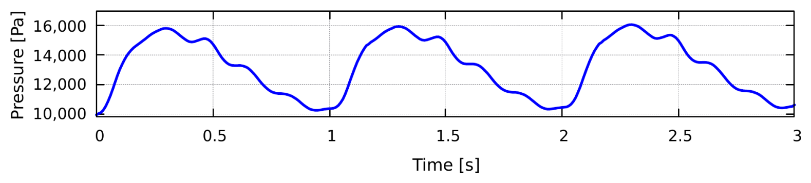
The adopted FSI strategy is partitioned strongly coupled, and the implicit Interface Quasi-Newton with Inverse Jacobian (IQNI) algorithm was employed to perform the coupled calculations [36]. An absolute convergence criterion based on the $L_2$ norm (of order 2) of the displacement residual at the interface has been imposed. The maximum number of FSI coupling iterations was set to 20 and the convergence is achieved when the residual value falls below the set tolerance, equal to $1\times {10}^{-5}$ m. A fixed time step of $1\times {10}^{-3}$ s was adopted for the FSI simulation, providing a reasonable computational cost whilst ensuring numerical stability, particularly given the very similar densities of the fluid and solid, incompressible fluid and the nearly incompressible behavior of the solid material [19]. The simulation was carried out up to the third cycle, which was taken as a reference for the physiological parameters analysed [37,42,48,49,83]. By the third cycle, the simulation reach stability (cf. Figure 7), as the difference between the pressures, calculated using the Equation (9), at the start of the cardiac cycle is less than $2\%$.

$$difference={\displaystyle \frac{P_{n+1}-P_n}{P_n}}<2\%$$

(9)

where $P_n$ denotes the initial average pressure at the nth cycle at section $S_3$.

The FSI simulation was performed using 22 cores, and it required about 500 core-hours to complete one cardiac cycle.

Using the same number of cores, the CFD simulation required about 100 core-hours. The FSI simulation required a computational cost 5 times greater than the CFD.

2.3.2. Boundary Condition

For the solid domain, the Outlet was constrained with zero displacement, whereas a radial displacement boundary condition was prescribed at the Inlet to permit radial deformation consistent with physiological wall compliance. Radial deformation, defined with respect to a local reference system, is not natively supported in Abaqus for non-axisymmetric geometries. Therefore, a custom Python, version 3.10, script was developed to compute the appropriate local reference system and to correctly apply this boundary condition.

Regarding the fluid domain, the pressure boundary condition shown in Figure 4a was imposed at the Outlet, while a velocity boundary condition was prescribed at the Inlet. The inlet velocity field, mapped from the rigid-wall CFD simulation, was appropriately scaled to account for the time-varying inlet area (Figure 2a) to maintain the exact same flow rate curve. This velocity vector rescaling was necessary due to the significant radial deformation of the inlet section.

3. Results and Discussion

Rigid-wall CFD and FSI simulations of a thoracic aorta affected by an aneurysm were compared to understand the numerical differences between the various physical quantities of interest, such as velocity, pressure, WSS, TAWSS, OSI and VMS. The following section presents these quantities in an orderly manner, highlighting the differences between CFD and FSI.

3.1. Velocity

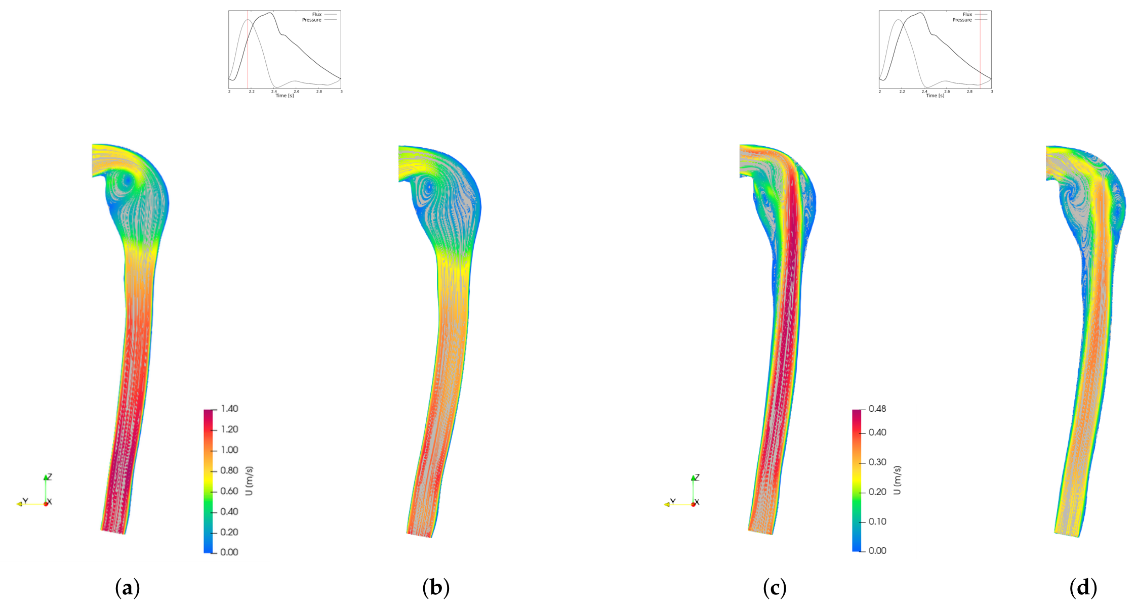
In Figure 8, some differences can be noted between the two types of simulations. At section $S_3$ (cf. Figure 3 for the location), the local maximum velocity is reached at the systolic peak, considered to be reached at the maximum flow peak with reference to the Figure 4b, $1.204$ m/s in the CFD simulation and $1.045$ m/s in the FSI simulation, corresponding to a increase of about ≃15% relative to the FSI result. During the diastolic phase, a maximum local velocity of $0.472$ m/s for CFD and $0.365$ m/s for FSI is obtained, with an increase of about ≃29% relative to FSI simulation. The maximum velocities are both reached in the DTA section at systolic peak. The result is consistent with the physics of the problem, as the cross-section area of the DTA part, in the FSI case, increases due to the internal pressure (Figure 3). In the FSI simulation, the area of the slice $S_3$ is equal to $2.34$ cm², while in CFD it is equal to $2.04$ cm², an increase of ≃12%. If we consider the average velocity calculated at systolic peak downstream of the aneurysm, represented by the box in Figure 3, as expected, the velocity is greater in the CFD case than in the FSI case, specifically $1.043$ m/s vs. $0.885$ m/s. During the diastolic phase, the velocity reaches $0.298$ m/s for the CFD simulation and $0.216$ m/s for the FSI simulation. These velocity values are consistent with the current literature in the case of DTAA [11,41].

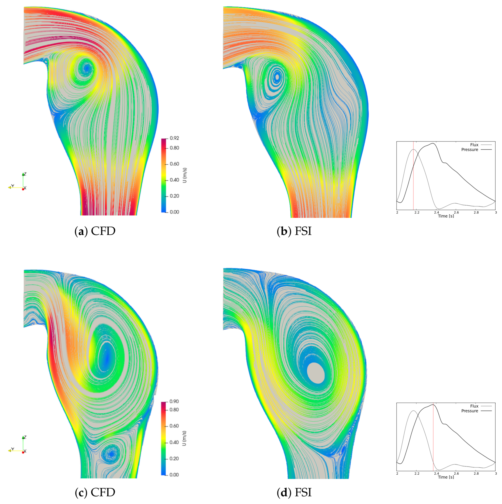
In both cases, given the presence of the aneurysm, there is strong recirculation of the blood within the bulge, as can be seen in Figure 9. The flow becomes disorganized and recirculation causes blood particles to remain in prolonged contact with the surface of the aneurysm, leading to potential platelet deposition on the surface [84]. Platelet deposition on the surface of the lumen contributes to thrombus formation.

3.2. Pressure

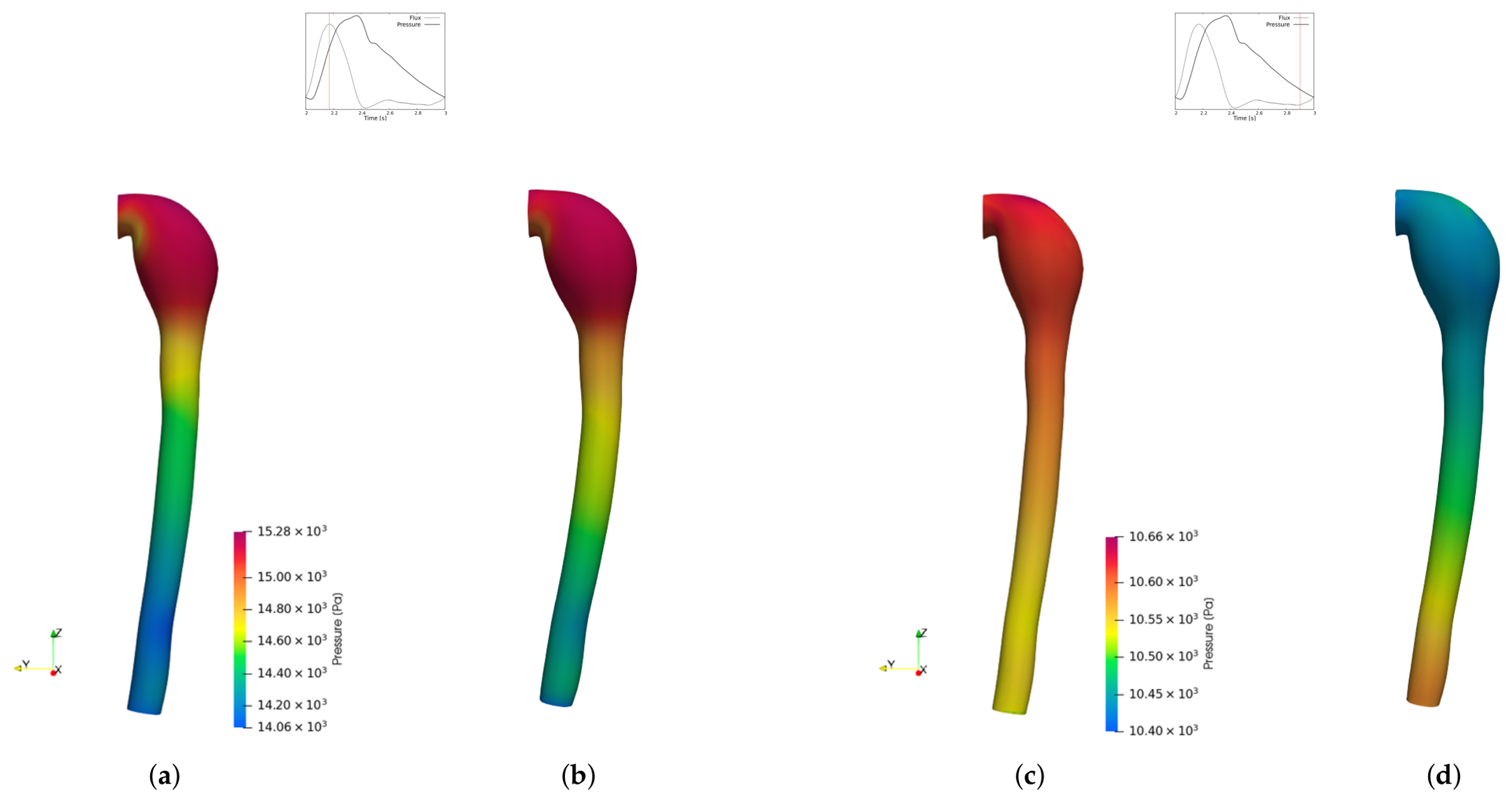
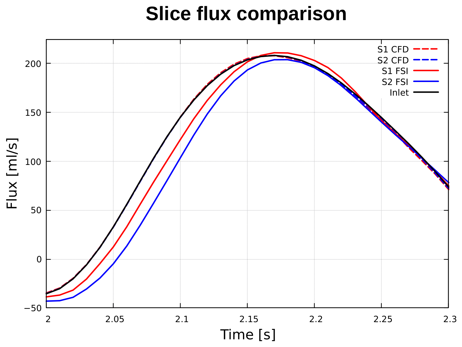
With regard to pressure, particularly with reference to Figure 10, a slightly higher pressure is observed in the FSI calculation compared to the CFD simulation during the systolic peak. This behaviour is due to the compliance of the deformable walls. In fact, as we can see from Figure 11, while in the CFD case the flows calculated in sections $S_1$ and $S_2$ coincide with the Inlet flow, in the FSI case there is a delay in the flow peak due to the deformation of the walls, which initially stores part of the inflowing volume. The aneurysm therefore acts as a flow accumulation zone until it reaches its maximum expansion limit. Thereafter, the pressure increases due to the incoming flow pushing the fluid already present inside the aneurysmal sac, against the distal narrowing, and due to the reaction of the deformable wall on the fluid, which releases the deformation energy previously stored. The characteristics of the material, in particular its low stiffness and uniform thickness, tends to accentuate the phenomenon just described. The deformation of sections, $S_1$ and $S_2$, shown in Figure 3, vary differently between the beginning of the cardiac cycle and the systolic peak by, $8\%$ and $5\%$ respectively, further confirming the accumulation zone behaviour exhibited by the aneurysm. Considering the diastolic phase, it can be seen that the percentage of deformation between sections $S_1$ and $S_2$ are substantially equal, thus causing a decrease in overall pressure in the FSI simulation compared to the CFD simulation. The average pressure across the entire domain at systolic peak is 14,797 Pa for the CFD calculation and 14,899 Pa for the FSI simulation. During the diastolic phase, instead, the CFD and FSI simulations yield values of 10,594 Pa and 10,464 Pa respectively. In both cases, low-pressure areas can be observed in the proximal and distal necks of the aneurysm, in agreement with [11,41].

3.3. Wall Shear Stress and Time Averaged Wall Shear Stress

WSS is one of the most important and analyzed parameters in this type of simulation, both in CFD and FSI [4]. WSS is defined as the tangential component of traction vector acting on the wall [37,42] and is calculated using Equation (10)

$$\mathbf{wss}=\mathbf{\tau }-(\mathbf{\tau }·\mathbf{n})\mathbf{n}$$

(10)

where $\mathbf{\tau }=\mu (\nabla \mathbf{u}+\nabla {\mathbf{u}}^T)\mathbf{n}$ is the traction vector due to shear stress and $\mu$ is the dynamic viscosity. In particular, a low value of WSS leads to an increased possibility of atherosclerotic plaque deposition, thrombosis, or vessel rupture [1,10,15,85].

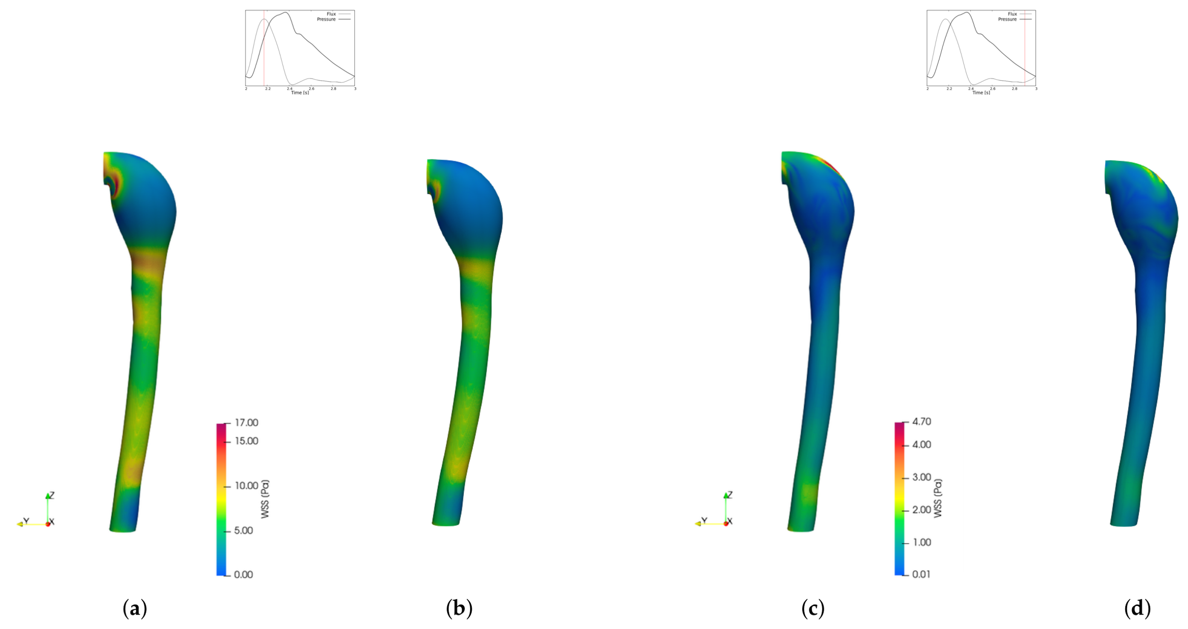
From Figure 12, it can be seen that the WSS distribution along the analyzed geometry is almost similar during the systolic peak. As for the diastolic phase, however, the WSS distribution varies more markedly, even within the aneurysm, compared to the systolic peak. The maximum average value of WSS at the systolic peak was found to be $5.730$ Pa for the CFD simulation and $4.751$ Pa for the FSI simulation. During the diastolic phase, the corresponding values were $0.876$ Pa for CFD and $0.671$ Pa for FSI. Overall, the rigid-wall CFD approach overestimates the WSS by approximately $21\%$ at systole and $31\%$ at diastole compared to the FSI calculation.

Another parameter investigated is TAWSS, which provides an overview of the entire cardiac cycle of WSS. TAWSS is calculated using the following definition

$$TAWSS={\displaystyle \frac{1}{T}}{\int }_0^T\left|\mathbf{wss}\right|dt$$

(11)

where T is the cardiac period.

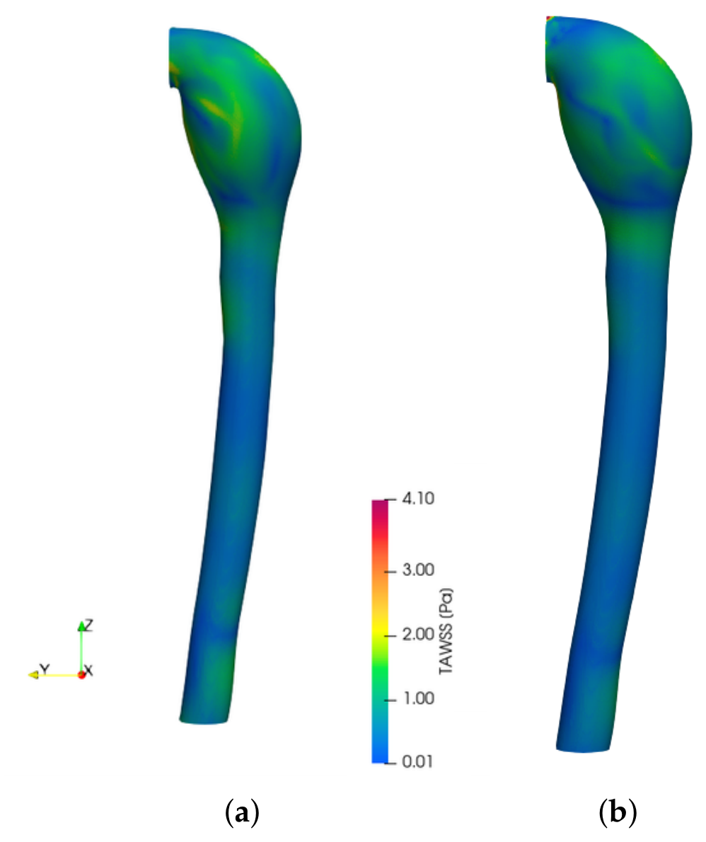
The TAWSS distributions obtained in the present study are shown in Figure 13. A high TAWSS value can lead to a greater risk of rupture of the affected walls [86], but reduces the risk of atherosclerosis and thrombus formation [87]. With reference to Figure 13, the TAWSS spatial distribution is similar between CFD and FSI with higher values in the proximal and distal parts of the aneurysm neck and also around the aneurysmal sac where the blood flow impinges on the aortic wall. Calculating the spatial mean of the TAWSS values over the entire surface yields $0.815$ Pa for the CFD case and $0.616$ Pa for the FSI case, i.e., an increase of approximately $32\%$ compared to the FSI simulation. However, compared to the previous overall value of the average spatial TAWSS relative to CFD, greater than in the FSI case, a higher local maximum is obtained in FSI, equal to $4.276$ Pa, compared to the CFD case, equal to $3.223$ Pa, located in the proximal part of the aneurysm. This behavior is due to the fact that deformation can deflect the flow in such a way that it impacts the walls more directly, effectively increasing the TAWSS value in specific areas.

3.4. OSI

The Oscillatory Shear Index (OSI) [88] is a parameter that quantifies the degree of directional oscillation of the WSS and is commonly used to identify areas of the artery subject to oscillatory flow, as defined in Equation (12).

$$OSI=0.5\left(1-{\displaystyle \frac{|{\int }_0^T\mathbf{wss}dt|}{{\int }_0^T\left|\mathbf{wss}\right|dt}}\right)$$

(12)

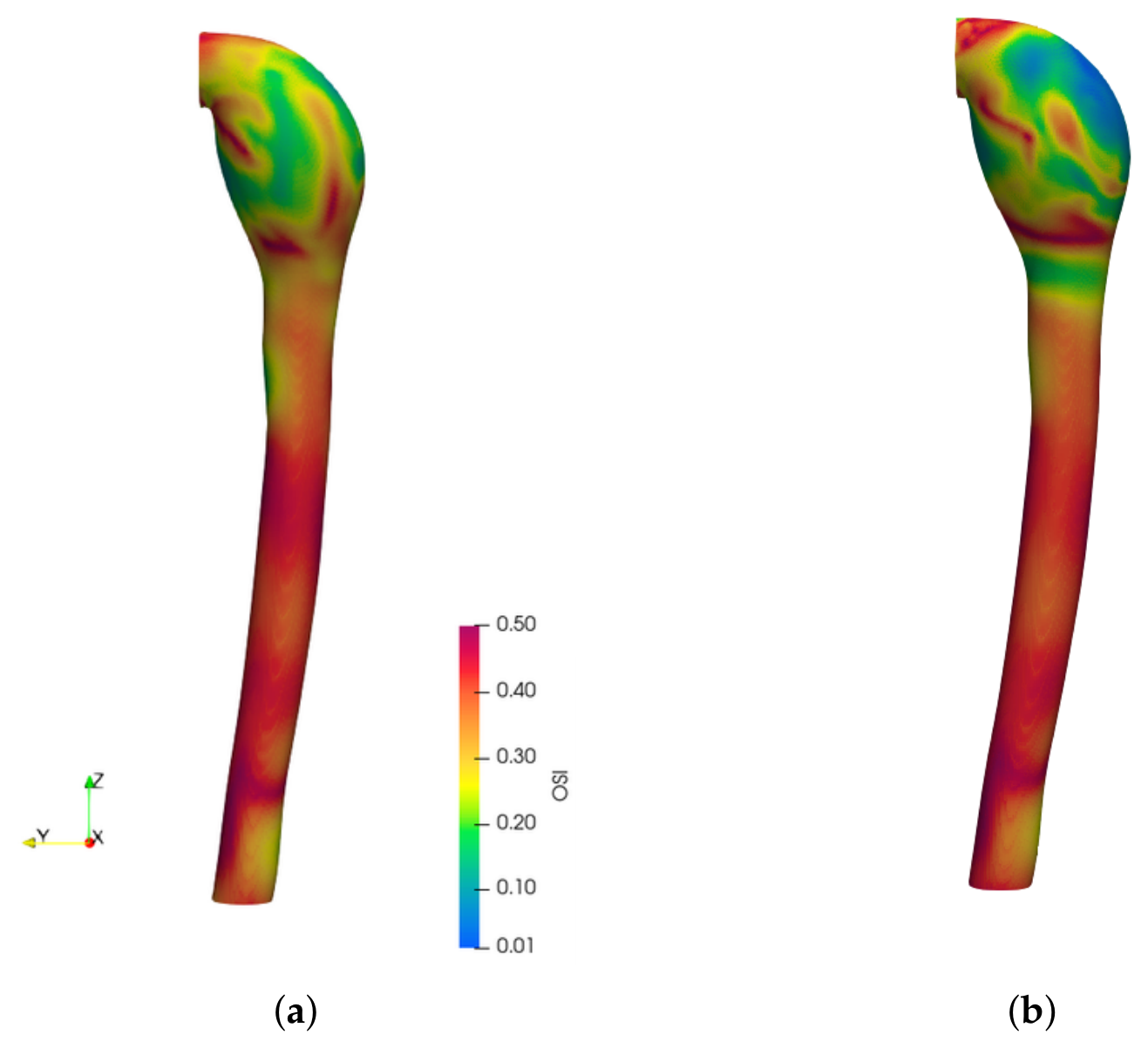
A value of $0.5$ corresponds to a purely oscillatory flow. With reference to Figure 14, it can be seen that OSI is elevated in the lateral and superior walls of the aneurysm, in accordance with the results described in [41,42]. High OSI values can lead to the formation of atherosclerosis and inflammation of the artery [89].

3.5. Wall Displacement

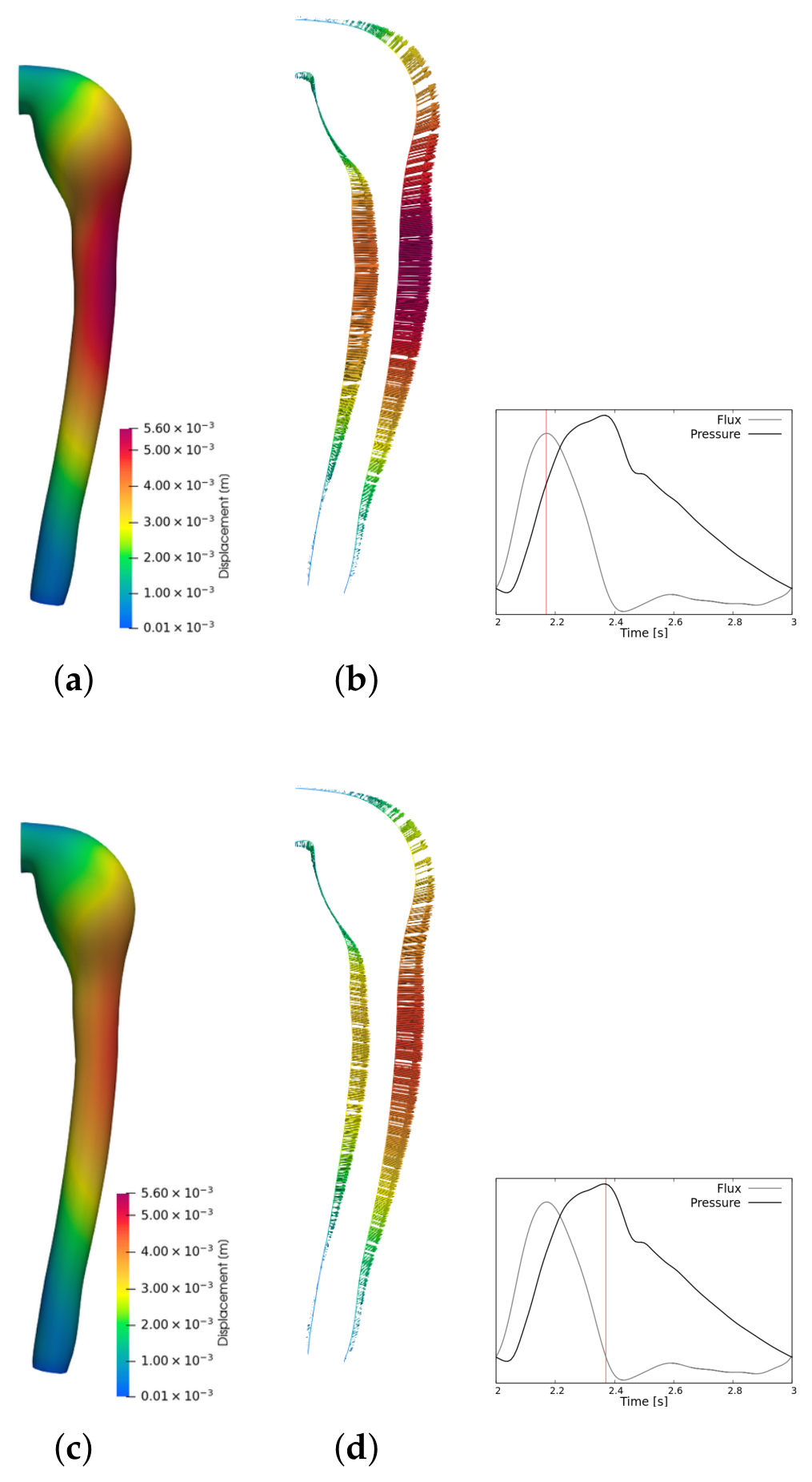
Figure 15 represents the displacement module on the surface and through the visualization of the vector itself on a slice, showing that the maximum displacement occurs at the systolic peak in the distal neck of the aneurysm. The maximum absolute displacement is $5.60$ mm. Considering section $S_1$ across the aneurysm (cf. Figure 3), the difference between the minimum and maximum equivalent diameter is approximately ≃1.54 mm, corresponding to an increase of $3.59\%$ between the systolic peak ($2.17$ s) and late diastole ($2.90$ s). The maximum displacement does not occur at the instant of maximum pressure but approximately at the systolic peak. This behavior is attributed to the transient nature of the flow and the associated inertial effects. In fact, as shown in Figure 9, the velocity in the outlet region of the aneurysm is higher at the systolic peak than at the pressure peak. The literature on DTAA wall displacement is currently limited; nevertheless, the present results are consistent in order of magnitude with those reported in existing studies [41,42].

3.6. Von Mises

Von Mises Stress (VMS), ${\sigma }_{vms}$, represents the equivalent stress and it is used as a scalar measure of the stress state in the aortic wall. Its definition is given by

$${\sigma }_{vms}=\sqrt{{\displaystyle \frac{{({\sigma }_I-{\sigma }_{II})}^2+{({\sigma }_{II}-{\sigma }_{III})}^2+{({\sigma }_I-{\sigma }_{III})}^2}{2}}}$$

(13)

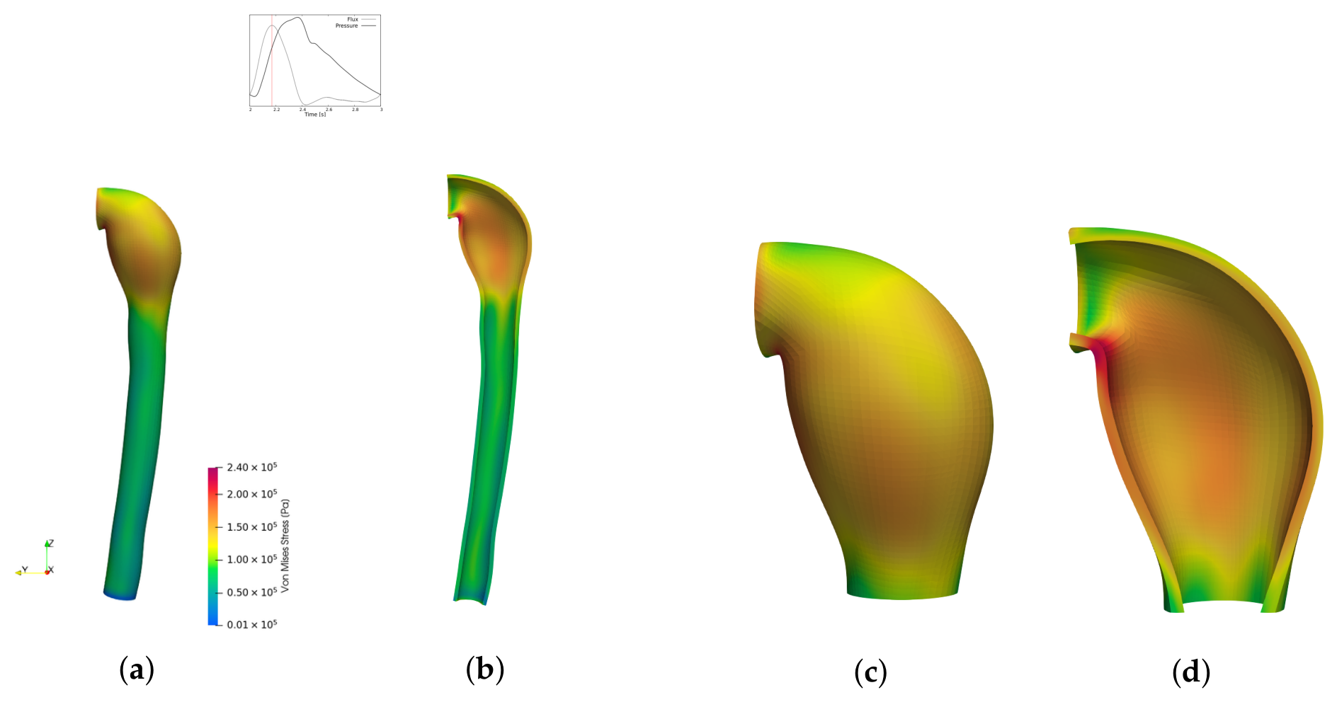
where ${\sigma }_i$ with $i=I,II,III$ denote the principal stresses of the Cauchy stress tensor. Figure 16 shows the VMS distribution over the entire geometry and within the aneurysm. The maximum value, equal to $0.235$ MPa, is observed in the region proximal to the aneurysm neck rather than within the DTA region. The highest stress levels occur in regions characterized by sharp geometric curvature, where stress concentrations are expected. As anticipated, the VMS remains well below reported rupture thresholds, according to experimental studies ranging from 0.8–2.3 MPa [90,91,92], and therefore does not indicate a risk of aneurysm rupture for the case study examined. It should also be noted that the aneurysmal region is subject to the greatest tensile loading due to the locally higher pressure levels (Figure 10).

3.7. Summary of Results

For further clarity, the main results regarding the comparison of hemodynamic parameters during the systolic peak are summarized in

Table 4. Peak systolic haemodynamic parameters. The difference, expressed as a percentage, is relative to the FSI case. $S_3$ refers to section shown in Figure 3.

Haemodynamic Parameters	CFD	FSI	Difference
Velocity $(S_3)\left[{\displaystyle \frac{\mathrm{m}}{\mathrm{s}}}\right]$	$1.204$	$1.045$	$15\%$
Pressure [Pa]	14,797	14,899	$-0.68\%$
WSS [Pa]	$5.730$	$4.751$	$21\%$

and

Table 5. Diastolic haemodynamic parameters. The difference, expressed as a percentage, is relative to the FSI case. $S_3$ refers to section shown in Figure 3.

Haemodynamic Parameters	CFD	FSI	Difference
Velocity $(S_3)\left[{\displaystyle \frac{\mathrm{m}}{\mathrm{s}}}\right]$	$0.472$	$0.365$	$29\%$
Pressure [Pa]	10,594	10,464	$1.24\%$
WSS [Pa]	$0.876$	$0.671$	$31\%$

.

The TAWSS parameter is a parameter computed within the cardiac cycle; in our case, the CFD calculation yields a value of $0.815$ Pa, whereas the FSI calculation yields a value of $0.616$ Pa, representing a $32\%$ increase compared to the FSI calculation.

Similarly to the hemodynamic parameters, the main results concerning the structural domain are summarized in

Table 6. FSI simulation structural parameter values. $S_1$ refers to section shown in Figure 3.

Structural Parameters	Value
Max Displacement [mm]	$5.60$
Max diameter difference ($S_1$) [mm]	$1.54$
Max VMS [MPa]	$0.235$

.

For the sake of completeness,

Table 7. Comparison of haemodynamic and structural parameters at systolic peak.

Haemodynamic and Structural Parameters	Present Study	Duca et al. [41]	Difference
${\displaystyle \frac{Velocit{y}_{DTA}}{Velocit{y}_{sac}}}$	$1.7$	$2.3$	$-26\%$
${\displaystyle \frac{Pressur{e}_{DTA}}{Pressur{e}_{sac}}}$	$1.017$	$1.016$	$0.1\%$
Max Displacement [mm]	$5.60$	$6.11$	$-8.35\%$
Max VMS [MPa]	$0.235$	$0.210$	$11\%$

present the values obtained in this study, along with the most recent paper on the DTAA case [41]. For the hemodynamic parameters, in order to compensate for differences in geometry, we use non-dimensional values: the ratio of the maximum velocity/pressure calculated within the aneurysm sac to the maximum velocity/pressure recorded in the DTA section. For structural quantities, instead, we used absolute values.

As can be seen, the velocity ratio shows a $26\%$ difference, but this is primarily due to the geometric difference at the aneurysm neck. For pressure, the difference is essentially zero, since pressure is dominated by the boundary conditions, supporting the accuracy of our simulation.

Table 7 shows also the structural values for the two cases. As can be seen, values for maximum displacement and VMS are of the same order of magnitude, with small deviations despite the different geometries since these quantities are primarily driven by pressure, as highlighted earlier.

4. Conclusions

In the present work, a comparison between rigid-wall CFD and FSI simulations of a DTAA is presented. Pulsatile flow was imposed as a boundary condition at the inlet, while a three-element Windkessel model, implemented in OpenFOAM, was applied as pressure boundary to the carotid and subclavian arteries; a prescribed pressure waveform was applied at the main outlet. Blood flow was modeled as laminar with the incompressible fluid assumption, and the arterial tissue was represented using a Neo-Hookean material model. The main findings can be summarized as follows:

• Higher velocity values were observed during both the systolic and diastolic phases in the CFD simulations compared with the FSI results.
• The pressure distribution is slightly higher in the FSI simulation than in the CFD case during the systolic peak, and, to the best of our knowledge, such aspect is not reported and discussed in the literature. During diastolic phase, the pressure is higher in the CFD simulation as expected and already reported.
• The WSS reflects the trends observed for velocity and pressure, with an increase of $21\%$ and $31\%$ for the CFD simulations compared to the FSI results during the systolic and diastolic phases, respectively.
• The spatial distribution of TAWSS is qualitatively similar between the CFD and FSI simulations; however, the CFD approach overestimates its magnitude by $32\%$ compared to the FSI calculation.
• The OSI reveals marked qualitative differences within the aneurysmal sac, highlighting the influence of wall compliance on local flow oscillations and shear reversal patterns that are not captured by rigid-wall CFD simulations.
• In the solid domain, the maximum displacement of the arterial tissues occurs in the distal region of the aneurysm neck, while the maximum variation in aneurysm diameter between systole and diastole remains below $5\%$. The VMS values are well below the material rupture limits.

The results highlight a significant sensitivity of pressure, wall deformation and stress distributions to the assumed mechanical properties of the arterial wall. The haemodynamic parameters described above, such as WSS and TAWSS, show significant differences between the CFD and FSI models due to the compliance not captured by the rigid-wall model. The aneurysmal sac is not a static tube but acts as a reservoir for blood flow. Thanks to its compliance, the wall expands during systole, storing blood volume and releasing it during diastole, a buffering effect that attenuates mechanical loads. This function is intrinsically related to the shape and volume of the bulge: the larger the aneurysm, the more the rigid model fails to capture this physics. Furthermore, CFD calculations alone do not allow for the analysis of wall deformation and associated stresses. Although no direct clinical validation is provided, these findings suggest that neglecting wall deformation may lead to non-negligible discrepancies in the estimation of haemodynamic quantities in DTAA, potentially affecting their interpretation in a clinical context.

Although the use of a Newtonian model to simulate the blood flow is acceptable, a non-Newtonian model could be used to obtain more realistic results, particularly within the aneurysm sac. In the solid domain a uniform wall thickness and a constant Young’s modulus were adopted in the study, the nature of the case analyzed suggests that spatially varying thickness and elastic properties may be required for further improving the realism of the simulations. Future developments will also take into account not only the inclusion of non-Newtonian fluids, but also the effects of external pressure and the forces arising from the surrounding and constraints on displacement in the common and subclavian arteries.

References

1. Katritsis, D.; Kaiktsis, L.; Chaniotis, A.; Pantos, J.; Efstathopoulos, E.P.; Marmarelis, V. Wall shear stress: Theoretical considerations and methods of measurement. Prog. Cardiovasc. Dis. 2007, 49, 307–329. [Google Scholar] [CrossRef] [PubMed]
2. Silverthorn, D.U. Human Physiology; Jones & Bartlett Publishers: Burlington, MA, USA, 2015. [Google Scholar]
3. Garamendi, P.M.; Lucena, J.S.; Gómez-Bueno, M.; Segovia, J. Pulmonary Artery Pathology. In Clinico-Pathological Atlas of Cardiovascular Diseases; Springer: Berlin/Heidelberg, Germany, 2014; pp. 31–52. [Google Scholar]
4. Saib, Z.A.; Abed, F.; Ghayesh, M.H.; Amabili, M. A Review of Fluid-Structure Interaction: Blood Flow in Arteries. Biomed. Eng. Adv. 2025, 9, 100171. [Google Scholar]
5. Natsume, K.; Shiiya, N.; Takehara, Y.; Sugiyama, M.; Satoh, H.; Yamashita, K.; Washiyama, N. Characterizing saccular aortic arch aneurysms from the geometry-flow dynamics relationship. J. Thorac. Cardiovasc. Surg. 2017, 153, 1413–1420.e1. [Google Scholar] [CrossRef] [PubMed]
6. Houriez-Gombaud-Saintonge, S.; Mousseaux, E.; Bargiotas, I.; De Cesare, A.; Dietenbeck, T.; Bouaou, K.; Redheuil, A.; Soulat, G.; Giron, A.; Gencer, U.; et al. Comparison of different methods for the estimation of aortic pulse wave velocity from 4D flow cardiovascular magnetic resonance. J. Cardiovasc. Magn. Reson. 2019, 21, 75. [Google Scholar] [CrossRef] [PubMed]
7. Yamaguchi, T.; Ishikawa, T.; ichi Tsubota, K.; Imai, Y.; Nakamura, M.; Fukui, T. Computational Blood Flow Analysis—New Trends and Methods. J. Biomech. Sci. Eng. 2006, 1, 29–50. [Google Scholar] [CrossRef]
8. Boussel, L.; Rayz, V.; Martin, A.; Acevedo-Bolton, G.; Lawton, M.T.; Higashida, R.; Smith, W.S.; Young, W.L.; Saloner, D. Phase-Contrast magnetic resonance imaging measurements in intra-cranial aneurysms in vivo of flow patterns, velocity fields, and wall shear stress: Comparison with CFD. Magn. Reson. Med. 2009, 61, 409–417. [Google Scholar] [CrossRef] [PubMed]
9. Biancolini, M.E.; Capellini, K.; Costa, E.; Groth, C.; Celi, S. Fast interactive CFD evaluation of hemodynamics assisted by RBF mesh morphing and reduced order models: The case of aTAA modelling. Int. J. Interact. Des. Manuf. (IJIDEM) 2020, 14, 1227–1238. [Google Scholar] [CrossRef]
10. Balasubramanya, A.; Maes, L.; Rega, F.; Mazzi, V.; Morbiducci, U.; Famaey, N.; Degroote, J.; Segers, P. Hemodynamics and wall shear metrics in a pulmonary autograft: Comparing a fluid-structure interaction and computational fluid dynamics approach. Comput. Biol. Med. 2024, 176, 108604. [Google Scholar] [CrossRef] [PubMed]
11. Silva, M.L.F.D.; Goncalves, S.D.F.; Haniel, J.; Lucas, T.C.; Huebner, R. Comparative study between 1-way and 2-way coupled fluid-structure interaction in numerical simulation of aortic arch aneurysms. An. Acad. Bras. Ciências 2023, 95, e20210859. [Google Scholar] [CrossRef]
12. Ene-Iordache, B. Descriptors of Flow in Computational Hemodynamics. Fluids 2025, 10, 191. [Google Scholar] [CrossRef]
13. Duronio, F.; Di Mascio, A. Blood Flow Simulation of Aneurysmatic and Sane Thoracic Aorta Using OpenFOAM CFD Software. Fluids 2023, 8, 272. [Google Scholar] [CrossRef]
14. Formaggia, L.; Quarteroni, A.; Veneziani, A. Cardiovascular Mathematics: Modeling and Simulation of the Circulatory System; Springer Science & Business Media: Berlin/Heidelberg, Germany, 2010; Volume 1. [Google Scholar]
15. Fry, D.L. Acute vascular endothelial changes associated with increased blood velocity gradients. Circ. Res. 1968, 22, 165–197. [Google Scholar] [CrossRef] [PubMed]
16. Duronio, F.; Marchetti, P. Investigation of the Pulmonary Artery Hypertension Using an Ad Hoc OpenFOAM CFD Solver. Fluids 2025, 10, 6. [Google Scholar] [CrossRef]
17. Richter, T. Fluid-Structure Interactions: Models, Analysis and Finite Elements; Cambridge University Press: Cambridge, UK, 2017. [Google Scholar]
18. Malvern, L.E. Introduction to the Mechanics of a Continuous Medium; Prentice-Hall: Englewood Cliffs, NJ, USA, 1969. [Google Scholar]
19. Degroote, J.; Bruggeman, P.; Haelterman, R.; Vierendeels, J. Stability of a coupling technique for partitioned solvers in FSI applications. Comput. Struct. 2008, 86, 2224–2234. [Google Scholar] [CrossRef]
20. Hou, T.; Wei, X.; Iqbal, A.; Yang, X.; Wang, J.; Ren, Y.; Yan, S. Advances in biomedical fluid–structure interaction: Methodologies and applications from an interfacing perspective. Phys. Fluids 2024, 36, 021301. [Google Scholar] [CrossRef]
21. Hughes, T.J.; Liu, W.K.; Zimmermann, T.K. Lagrangian-Eulerian finite element formulation for incompressible viscous flows. Comput. Methods Appl. Mech. Eng. 1981, 29, 329–349. [Google Scholar] [CrossRef]
22. Donea, J.; Giuliani, S.; Halleux, J.P. An arbitrary Lagrangian-Eulerian finite element method for transient dynamic fluid-structure interactions. Comput. Methods Appl. Mech. Eng. 1982, 33, 689–723. [Google Scholar] [CrossRef]
23. Figueroa, C.A.; Vignon-Clementel, I.E.; Jansen, K.E.; Hughes, T.J.; Taylor, C.A. A coupled momentum method for modeling blood flow in three-dimensional deformable arteries. Comput. Methods Appl. Mech. Eng. 2006, 195, 5685–5706. [Google Scholar] [CrossRef]
24. Richter, T. A fully Eulerian formulation for fluid–structure-interaction problems. J. Comput. Phys. 2013, 233, 227–240. [Google Scholar] [CrossRef]
25. Laadhari, A. Implicit finite element methodology for the numerical modeling of incompressible two-fluid flows with moving hyperelastic interface. Appl. Math. Comput. 2018, 333, 376–400. [Google Scholar] [CrossRef]
26. Taelman, L.; Bols, J.; Degroote, J.; Muthurangu, V.; Panzer, J.; Vierendeels, J.; Segers, P. Differential impact of local stiffening and narrowing on hemodynamics in repaired aortic coarctation: An FSI study. Med. Biol. Eng. Comput. 2016, 54, 497–510. [Google Scholar] [PubMed]
27. Campobasso, R.; Condemi, F.; Viallon, M.; Croisille, P.; Campisi, S.; Avril, S. Evaluation of peak wall stress in an ascending thoracic aortic aneurysm using FSI simulations: Effects of aortic stiffness and peripheral resistance. Cardiovasc. Eng. Technol. 2018, 9, 707–722. [Google Scholar] [CrossRef] [PubMed]
28. Avril, S.; Goriely, A.; Holzapfel, G.A.; Kuhl, E.; Nordsletten, D.; Ogden, R.W. State-of-the-art and tomorrow’s challenges and opportunities in constitutive modeling of soft biological tissues with a focus on arterial, cardiac and brain biomechanics. Acta Biomater. 2026, 213, 62–87. [Google Scholar] [PubMed]
29. Liang, L.; Mao, W.; Sun, W. A feasibility study of deep learning for predicting hemodynamics of human thoracic aorta. J. Biomech. 2020, 99, 109544. [Google Scholar] [CrossRef] [PubMed]
30. Lin, D.; Westenberg, J.; Lamb, H.; Kenjereš, S. MRI-based CFD simulations of transient blood flow in compliant aortas using the LDDMM framework. Comput. Methods Programs Biomed. 2026, 282, 109385. [Google Scholar] [CrossRef] [PubMed]
31. Suk, J.; Alblas, D.; Hutten, B.; Wiegman, A.; Brune, C.; Van Ooij, P.; Wolterink, J.M. Physics-informed graph neural networks for flow field estimation in carotid arteries. Med. Image Anal. 2026, 110, 103974. [Google Scholar] [CrossRef] [PubMed]
32. Lin, D.; Kenjereš, S. Towards fast and reliable estimations of 3D pressure, velocity and wall shear stress in aortic blood flow: CFD-based machine learning approach. Comput. Biol. Med. 2025, 191, 110137. [Google Scholar] [CrossRef] [PubMed]
33. Rehman, M.A.U.; Ekici, Ö.; Farooq, M.A.; Talha, R.M.; Amir, S. Application of computational fluid dynamics and physics informed neural networks in predicting rupture risk of thoracoabdominal aneurysms with fluid-structure interaction analysis. Chin. J. Phys. 2025, 95, 433–454. [Google Scholar] [CrossRef]
34. Jinendran, C. Fluid Structure Interaction: A Brief Review. 2020. Available online: https://figshare.com/articles/journal_contribution/Review_of_FSI_Methods/12156741?file=22354563 (accessed on 2 July 2026).
35. Yue, X.; Huang, J.; Liu, J. Fluid-structure interaction analysis for abdominal aortic aneurysms: The role of multi-layered tissue architecture and intraluminal thrombus. Front. Bioeng. Biotechnol. 2025, 13, 1519608. [Google Scholar] [CrossRef] [PubMed]
36. Degroote, J.; Haelterman, R.; Annerel, S.; Bruggeman, P.; Vierendeels, J. Performance of partitioned procedures in fluid–structure interaction. Comput. Struct. 2010, 88, 446–457. [Google Scholar] [CrossRef]
37. Crosetto, P.; Reymond, P.; Deparis, S.; Kontaxakis, D.; Stergiopulos, N.; Quarteroni, A. Fluid–structure interaction simulation of aortic blood flow. Comput. Fluids 2011, 43, 46–57. [Google Scholar] [CrossRef]
38. Scotti, C.M.; Shkolnik, A.D.; Muluk, S.C.; Finol, E.A. Fluid-structure interaction in abdominal aortic aneurysms: Effects of asymmetry and wall thickness. Biomed. Eng. Online 2005, 4, 64. [Google Scholar] [CrossRef] [PubMed]
39. Di Martino, E.S.; Guadagni, G.; Fumero, A.; Ballerini, G.; Spirito, R.; Biglioli, P.; Redaelli, A. Fluid-structure interaction within realistic three-dimensional models of the aneurysmatic aorta as a guidance to assess the risk of rupture. Med. Eng. Phys. 2001, 23, 647–655. [Google Scholar] [CrossRef] [PubMed]
40. Petuchova, A.; Maknickas, A. Computational analysis of aortic haemodynamics in the presence of ascending aortic aneurysm. Technol. Health Care 2021, 29, 1079–1088. [Google Scholar] [CrossRef] [PubMed]
41. Duca, F.; Bissacco, D.; Crugnola, L.; Faitini, C.; Domanin, M.; Migliavacca, F.; Trimarchi, S.; Vergara, C. Computational analysis to assess hemodynamic forces in descending thoracic aortic aneurysms. J. Physiol. 2025. epub ahead of print. [Google Scholar] [CrossRef] [PubMed]
42. Tan, F.; Torii, R.; Borghi, A.; Mohiaddin, R.; Wood, N.; Xu, X. Fluid-structure interaction analysis of wall stress and flow patterns in a thoracic aortic aneurysm. Int. J. Appl. Mech. 2009, 1, 179–199. [Google Scholar] [CrossRef]
43. de Hart, J.; Peters, G.W.M.; Schreurs, P.J.G.; Baaijens, F.P.T. A three-dimensional computational analysis of fluid-structure interaction in the aortic valve. J. Biomech. 2003, 36, 103–112. [Google Scholar] [CrossRef] [PubMed]
44. Ghasemi Pour, M.; Zare, A.; Riasi, A. Modeling of aortic valve stenosis using fluid-structure interaction method. Comput. Biol. Med. 2021, 134, 104460. [Google Scholar] [CrossRef] [PubMed]
45. Yin, Z.; Armour, C.; Kandail, H.; O’Regan, D.P.; Bahrami, T.; Mirsadraee, S.; Pirola, S.; Xu, X.Y. Fluid–structure interaction analysis of a healthy aortic valve and its surrounding haemodynamics. Int. J. Numer. Methods Biomed. Eng. 2024, 40, e3865. [Google Scholar] [CrossRef] [PubMed]
46. Cao, K.; Sucosky, P. Effect of Bicuspid Aortic Valve Cusp Fusion on Aorta Wall Shear Stress: Preliminary Computational Assessment and Implication for Aortic Dilation. World J. Cardiovasc. Dis. 2015, 5, 129–140. [Google Scholar] [CrossRef][Green Version]
47. Criseo, E.; Fumagalli, I.; Quarteroni, A.; Marianeschi, S.M.; Vergara, C. Computational haemodynamics for pulmonary valve replacement by means of a reduced fluid–structure interaction model. Int. J. Numer. Methods Biomed. Eng. 2024, 40, e3846. [Google Scholar] [CrossRef] [PubMed]
48. Reymond, P.; Crosetto, P.; Deparis, S.; Quarteroni, A.; Stergiopulos, N. Physiological simulation of blood flow in the aorta: Comparison of hemodynamic indices as predicted by 3-D FSI, 3-D rigid wall and 1-D models. Med. Eng. Phys. 2013, 35, 784–791. [Google Scholar] [PubMed]
49. Mendez, V.; Di Giuseppe, M.; Pasta, S. Comparison of hemodynamic and structural indices of ascending thoracic aortic aneurysm as predicted by 2-way FSI, CFD rigid wall simulation and patient-specific displacement-based FEA. Comput. Biol. Med. 2018, 100, 221–229. [Google Scholar] [PubMed]
50. Hu, M.; Chen, B.; Luo, Y. Computational fluid dynamics modelling of hemodynamics in aortic aneurysm and dissection: A review. Front. Bioeng. Biotechnol. 2025, 13, 1556091. [Google Scholar] [CrossRef] [PubMed]
51. Mourato, A.; Valente, R.; Xavier, J.; Brito, M.; Avril, S.; de Sa, J.C.; Tomas, A.; Fragata, J. Computational modelling and simulation of fluid structure interaction in aortic aneurysms: A systematic review and discussion of the clinical potential. Appl. Sci. 2022, 12, 8049. [Google Scholar] [CrossRef]
52. Pons, R.; Guala, A.; Rodríguez-Palomares, J.F.; Cajas, J.; Dux-Santoy, L.; Teixidó-Tura, G.; Molins, J.J.; Vázquez, M.; Evangelista, A.; Martorell, J. Fluid–structure interaction simulations outperform computational fluid dynamics in the description of thoracic aorta haemodynamics and in the differentiation of progressive dilation in Marfan syndrome patients. R. Soc. Open Sci. 2020, 7, 191752. [Google Scholar] [CrossRef] [PubMed]
53. Dell’Agnello, F.; Capellini, K.; Gasparotti, E.; Scarpolini, M.A.; Buongiorno, R.; Monteleone, A.; Cademartiri, F.; Celi, S. Towards patient-specific hemodynamics of the aorta: A comprehensive CT-guided approach for moving boundary CFD simulations. Comput. Biol. Med. 2025, 198, 111202. [Google Scholar] [CrossRef] [PubMed]
54. Tabatabaeishoorijeh, S. A Comparison of FSI Modeling to Rigid-Wall CFD in Aortic Dissection. Proc. Tex. A&M Med. Stud. Grand Rounds 2023. Available online: https://jmsgr.tamhsc.edu/surgical-augmentation-of-rotator-cuff-repair/ (accessed on 2 July 2026).
55. Mahjoub, H.; Hassani, K.; Sheikhani, A.; Razeghi, M. Computational fluid–structure interaction analysis of arterial hemodynamics for cardiovascular risk assessment. Comput. Methods Biomech. Biomed. Eng. 2025. [Google Scholar] [CrossRef] [PubMed]
56. Tricarico, R.; Berceli, S.A.; Tran-Son-Tay, R.; He, Y. Non-invasive estimation of the parameters of a three-element windkessel model of aortic arch arteries in patients undergoing thoracic endovascular aortic repair. Front. Bioeng. Biotechnol. 2023, 11, 1127855. [Google Scholar] [CrossRef] [PubMed]
57. Wilson, N.M.; Ortiz, A.K.; Johnson, A.B. The vascular model repository: A public resource of medical imaging data and blood flow simulation results. J. Med. Devices 2013, 7, 040923. [Google Scholar] [CrossRef]
58. Juretic, F. cfMesh User Guide. 2015. Available online: https://cfmesh.com/wp-content/uploads/2015/09/User_Guide-cfMesh_v1.1.pdf (accessed on 2 July 2026).
59. Celik, I.B.; Ghia, U.; Roache, P.J.; Freitas, C.J. Procedure for estimation and reporting of uncertainty due to discretization in CFD applications. J. Fluids Eng.-Trans. ASME 2008, 130, 071401. [Google Scholar] [CrossRef]
60. Gasser, T.C.; Avril, S.; Elefteriades, J.A. Biomechanics of the Aorta: Modeling for Patient Care; Elsevier: Amsterdam, The Netherlands, 2024. [Google Scholar]
61. Wu, T.; Zhu, H.; Zhuo, H.; Li, J.; Xiao, J. Fluid-structure interaction study of penetrating atherosclerotic ulcers: Assessing progression and rupture risks. Comput. Methods Programs Biomed. 2025, 270, 108973. [Google Scholar] [CrossRef] [PubMed]
62. Minniti, M.; Gramigna, V.; Palumbo, A.; Fragomeni, G. Application of Mathematical Models for Blood Flow in Aorta and Right Coronary Artery. Appl. Sci. 2025, 15, 5748. [Google Scholar] [CrossRef]
63. Isaksen, J.G.; Bazilevs, Y.; Kvamsdal, T.; Zhang, Y.; Kaspersen, J.H.; Waterloo, K.; Romner, B.; Ingebrigtsen, T. Determination of wall tension in cerebral artery aneurysms by numerical simulation. Stroke 2008, 39, 3172–3178. [Google Scholar] [CrossRef] [PubMed]
64. Berguer, R.; Bull, J.L.; Khanafer, K. Refinements in mathematical models to predict aneurysm growth and rupture. Ann. N. Y. Acad. Sci. 2006, 1085, 110–116. [Google Scholar] [CrossRef] [PubMed]
65. Nerem, R.; Seed, W.; Wood, N. An experimental study of the velocity distribution and transition to turbulence in the aorta. J. Fluid Mech. 1972, 52, 137–160. [Google Scholar] [CrossRef]
66. Morris, L.; Delassus, P.; Callanan, A.; Walsh, M.; Wallis, F.; Grace, P.; McGloughlin, T. 3-D numerical simulation of blood flow through models of the human aorta. J. Biomech. Eng. 2005, 127, 767–775. [Google Scholar] [CrossRef] [PubMed]
67. Boyd, J.; Buick, J. Comparison of Newtonian and non-Newtonian flows in a two-dimensional carotid artery model using the lattice Boltzmann method. Phys. Med. Biol. 2007, 52, 6215. [Google Scholar] [PubMed]
68. Westerhof, N.; Lankhaar, J.-W.; Westerhof, B.E. The arterial Windkessel. Med. Biol. Eng. Comput. 2009, 47, 131–141. [Google Scholar] [CrossRef] [PubMed]
69. Lungu, A.; Wild, J.; Capener, D.; Kiely, D.; Swift, A.; Hose, D. MRI model-based non-invasive differential diagnosis in pulmonary hypertension. J. Biomech. 2014, 47, 2941–2947. [Google Scholar] [CrossRef] [PubMed]
70. Pochet, T.; Gerard, P.; Marnette, J.M.; D’orio, V.; Marcelle, R.; Fatemi, M.; Fossion, A.; Juchmes, J. Identification of three-element windkessel model: Comparison of time and frequency domain techniques. Arch. Int. Physiol. Biochim. Biophys. 1992, 100, 295–301. [Google Scholar] [CrossRef] [PubMed]
71. Weller, H.G.; Tabor, G.; Jasak, H.; Fureby, C. A tensorial approach to computational continuum mechanics using object-oriented techniques. Comput. Phys. 1998, 12, 620–631. [Google Scholar] [CrossRef]
72. Rotsaert, R.; Bollens, J.; Bral, A.; Famaey, N.; Degroote, J.; Segers, P. Development of a Fluid-Structure-Growth Framework for Aortic Adaptation in Healthy Ageing. In Proceedings of the 22nd National Day of Biomedical Engineering 2025, Brussels, Belgium, 5 December 2025. [Google Scholar]
73. Wilcox, D.C. Turbulence Modeling for CFD; DCW Industries: La Canada, CA, USA, 1998; Volume 2. [Google Scholar]
74. Delaissé, N.; Demeester, T.; Haelterman, R.; Degroote, J. Quasi-Newton methods for partitioned simulation of fluid–structure interaction reviewed in the generalized Broyden framework. Arch. Comput. Methods Eng. 2023, 30, 3271–3300. [Google Scholar]
75. Systèmes, D. Abaqus Documentation. Dassault Systèmes, Providence, RI. 2014. Available online: https://www.3ds.com/support/documentation/user-guides (accessed on 2 July 2026).
76. Issakhov, A.; Sabyrkulova, A.; Abylkassymova, A. The fluid-structure interaction during blood flow in a flexible stenotic thoracic aorta: Numerical study. Comput. Math. Appl. 2024, 165, 39–51. [Google Scholar] [CrossRef]
77. Amabili, M.; Asgari, M.; Breslavsky, I.D.; Franchini, G.; Giovanniello, F.; Holzapfel, G.A. Microstructural and mechanical characterization of the layers of human descending thoracic aortas. Acta Biomater. 2021, 134, 401–421. [Google Scholar] [CrossRef] [PubMed]
78. Holzapfel, G.A.; Gasser, T.C.; Ogden, R.W. A new constitutive framework for arterial wall mechanics and a comparative study of material models. J. Elast. Phys. Sci. Solids 2000, 61, 1–48. [Google Scholar] [CrossRef]
79. Gheysen, L.; Maes, L.; Famaey, N.; Segers, P. Pulse wave velocity: A clinical measure to aid material parameter estimation in computational arterial biomechanics. J. Biomech. 2023, 149, 111482. [Google Scholar] [CrossRef] [PubMed]
80. Wang, X.; Carpenter, H.J.; Ghayesh, M.H.; Kotousov, A.; Zander, A.C.; Amabili, M.; Psaltis, P.J. A review on the biomechanical behaviour of the aorta. J. Mech. Behav. Biomed. Mater. 2023, 144, 105922. [Google Scholar] [CrossRef] [PubMed]
81. Simo, J.C.; Hughes, T.J. Computational Inelasticity; Springer: Berlin/Heidelberg, Germany, 1998. [Google Scholar]
82. Ebrahimi, S.; Fallah, F. Investigation of coronary artery tortuosity with atherosclerosis: A study on predicting plaque rupture and progression. Int. J. Mech. Sci. 2022, 223, 107295. [Google Scholar] [CrossRef]
83. Zhu, Y.; Armour, C.; Li, B.; Pirola, S.; Salmasi, Y.; Athanasiou, T.; O’Regan, D.P.; Xu, X.Y. A combined 4D flow MR imaging and fluid–structure interaction analysis of ascending thoracic aortic aneurysms. Biomech. Model. Mechanobiol. 2025, 24, 829. [Google Scholar] [CrossRef] [PubMed]
84. Bluestein, D.; Niu, L.; Schoephoerster, R.T.; Dewanjee, M. Steady flow in an aneurysm model: Correlation between fluid dynamics and blood platelet deposition. J. Biomech. Eng. 1996, 118, 280–286. [Google Scholar] [CrossRef] [PubMed]
85. Roy, M.; Chakraborty, S. How does the stiffness of blood vessel walls and deposited plaques impact coronary artery diseases? Phys. Fluids 2024, 36, 081917. [Google Scholar] [CrossRef]
86. Condemi, F.; Campisi, S.; Viallon, M.; Croisille, P.; Avril, S. Relationship between ascending thoracic aortic aneurysms hemodynamics and biomechanical properties. IEEE Trans. Biomed. Eng. 2019, 67, 949–956. [Google Scholar] [CrossRef] [PubMed]
87. Zhan, J.M.; Lu, T.D.; Yang, Z.Y.; Hu, W.Q.; Su, W. Influence of the flow field and vortex structure of patient-specific abdominal aortic aneurysm with intraluminal thrombus on the arterial wall. Eng. Appl. Comput. Fluid Mech. 2022, 16, 2100–2122. [Google Scholar] [CrossRef]
88. Ku, D.N.; Giddens, D.P.; Zarins, C.K.; Glagov, S. Pulsatile flow and atherosclerosis in the human carotid bifurcation. Positive correlation between plaque location and low oscillating shear stress. Arterioscler. Off. J. Am. Heart Assoc. Inc. 1985, 5, 293–302. [Google Scholar] [CrossRef]
89. Mutlu, O.; Salman, H.E.; Al-Thani, H.; El-Menyar, A.; Qidwai, U.A.; Yalcin, H.C. How does hemodynamics affect rupture tissue mechanics in abdominal aortic aneurysm: Focus on wall shear stress derived parameters, time-averaged wall shear stress, oscillatory shear index, endothelial cell activation potential, and relative residence time. Comput. Biol. Med. 2023, 154, 106609. [Google Scholar] [CrossRef] [PubMed]
90. Mohan, D.; Melvin, J.W. Failure properties of passive human aortic tissue. I—Uniaxial tension tests. J. Biomech. 1982, 15, 887–902. [Google Scholar] [CrossRef] [PubMed]
91. Sherifova, S.; Holzapfel, G.A. Biomechanics of aortic wall failure with a focus on dissection and aneurysm: A review. Acta Biomater. 2019, 99, 1–17. [Google Scholar] [CrossRef] [PubMed]
92. Li, Z.; Pei, M.; Zhang, J.; Liu, N.; Wang, J.; Zou, D. A study to characterize the mechanical properties and material constitution of adult descending thoracic aorta based on uniaxial tensile test and digital image correlation. Front. Bioeng. Biotechnol. 2023, 11, 1178199. [Google Scholar] [CrossRef] [PubMed]
Figure 1. Geometry of the thoracic aorta affected by aneurysm shown from (a,b) two different perspectives.
Fluids 11 00171 g001
Figure 2. Surface and mesh used for the CFD simulation. (a) The names of the various arteries, here considered Outlet for the numerical simulation, are also shown, namely Right Subclavian Artery (RSA), Right Common Carotid Artery (RCCA), Left Subclavian Artery (LSA) and Left Common Carotid Artery (LCCA). (b) Mesh Zoom of the carotid and subclavian artery. (c) Mesh Zoom of the bottom of Descending thoracic aorta (DTA) in correspondence of Outlet.
Fluids 11 00171 g002
Figure 3. Slices and section of interest. Overview of the slice considered for the calculation of the area ( S 2 and S 3 ) and subsequently for calculating the variation of the diameter in time ( S 1 ). The box is the region for the grid convergence study.
Fluids 11 00171 g003
Figure 4. Boundary conditions. (a) Pulsatile pressure waveform imposed at the descending aortic outlet Outlet. (b) Pulsatile flux prescribed at the Inlet.
Fluids 11 00171 g004
Figure 5. Representation of the fluid domain used for the FSI simulation, highlighting the new inlet, Inlet, where the mapped velocity profile was applied (cf. geometry shown in Figure 2a). Overview of the fluid domain (a). Mesh details of the aneurysm zone (b) and DTA bottom part (c).
Fluids 11 00171 g005
Figure 6. Solid domain and mesh. Overview of the solid domain (a). Mesh details of the aneurysm zone (b) and DTA bottom part (c).
Fluids 11 00171 g006
Figure 7. History of the average pressure at S 3 in Figure 3.
Fluids 11 00171 g007
Figure 8. Velocity-magnitude streamlines. Comparison between CFD and FSI results at systolic peak in (a,b) and at diastole in (c,d). The vertical red line in the image above represents the time instant analyzed within the cardiac cycle, here and in all subsequent figures.
Fluids 11 00171 g008
Figure 9. Velocity-magnitude streamlines within the aneurysm region. Comparison between CFD and FSI results at systolic peak in (a,b) and at pressure peak in (c,d).
Fluids 11 00171 g009
Figure 10. Pressure fields. Comparison between CFD and FSI results at systolic peak in (a,b) and at diastole in (c,d).
Fluids 11 00171 g010
Figure 11. Comparison between Inlet flow and calculated flow in sections S 1 and S 2 .
Fluids 11 00171 g011
Figure 12. Wall Shear Stress fields. Comparison between CFD and FSI results at systolic peak in (a,b) and at diastole in (c,d).
Fluids 11 00171 g012
Figure 13. Time-averaged Wall Shear Stress. Comparison between CFD (a) and FSI (b) results.
Fluids 11 00171 g013
Figure 14. Oscillatory Shear Index. Comparison between CFD (a) and FSI (b) results.
Fluids 11 00171 g014
Figure 15. Displacement magnitude FSI simulation results. (a,b) at systolic peak, (c,d) at pressure peak.
Fluids 11 00171 g015
Figure 16. Von Mises Stress fields. FSI results at systolic peak. Overview of the external solid region (a). Overview cut of the solid region (b). Corresponding close-up view (c) and cut (d) on the aneurysm walls.
Fluids 11 00171 g016