Article

Numerical Simulation of Shock Wave Propagation Through Multiple Raindrops

1
School of Mechanics and Engineering Science, Shanghai University, No. 149 Yanchang Road, Jing’an District, Shanghai 200072, China
2
Hangzhou International Innovation Institute, Beihang University, Hangzhou 311115, China
3
School of Aeronautics and Astronautics, Shanghai Jiaotong University, Shanghai 200240, China
*
Authors to whom correspondence should be addressed.
Fluids 2026, 11(6), 152; https://doi.org/10.3390/fluids11060152
Submission received: 14 May 2026 / Revised: 7 June 2026 / Accepted: 13 June 2026 / Published: 16 June 2026
(This article belongs to the Special Issue Innovations in Multiphase Flow)

Abstract

A numerical study of shock wave propagation through multiple raindrops is presented using a density-based compressible two-phase flow solver coupled with a sharp-interface volume-of-fluid (VoF) method. The piecewise linear interface calculation (PLIC) approach is employed to reconstruct gas–liquid interfaces and capture droplet deformation during shock interaction. The numerical framework is first validated using a one-dimensional gas–liquid shock tube problem and a shock–helium bubble interaction benchmark. The method is then applied to investigate shock interactions with single, double, and multiple raindrops under compressible flow conditions. Numerical results show that complex wave structures, including shock reflection, diffraction, and wave interference, develop during shock propagation through raindrop fields. Interactions between neighboring droplets lead to local pressure amplification and non-uniform flow structures.

1. Introduction

Shock waves interacting with liquid droplets arise in a wide variety of environments, including transonic/supersonic flight through precipitation, detonation–droplet interaction, and high-speed propulsion systems. In particular, aircraft operating in rainy weather inevitably encounter raindrops and shock wave interactions.
Numerous works have been carried out to study the interactions between shock waves and droplets [1,2,3,4]. Experiments using shock tubes and high-speed imaging have revealed that the breakup behavior strongly depends on the Mach number and the pressure loading across the interface [5,6,7]. Despite these advances, experimental approaches remain limited in their ability to capture the detailed wave structure and droplets interaction. Since the characteristic timescales of these problems are extremely short, and the spatial scales are often very small, most experimental measurements focus on macroscopic quantities such as droplet shape and breakup patterns [3,8], while detailed flow information such as pressure distribution, wave propagation and local Mach number remains difficult to obtain. Consequently, numerical simulations have become an essential tool to investigate the interactions between shock waves and droplets.
Numerical simulations of compressible multiphase flows have advanced significantly over the past years [9,10,11,12,13,14,15,16,17,18,19]. Existing computational methods can be classified into two categories: diffuse-interface method and sharp-interface method. Diffuse-interface method represents the gas–liquid interface as a mixture region with finite thickness over several computational cells [20]. This method is robust and widely used in compressible multiphase flow simulations. However, the smeared representation of the interface often result in loss of geometric accuracy, particularly in flows involving strong shock waves and large density ratios. Under such conditions, accurately capturing interface shape becomes challenging.
Sharp-interface method treats the interface as a discontinuity and explicitly reconstructs its geometry [21]. Approaches such as level-set [22,23,24], coupled volume-of-fluid (VoF) [25,26,27] and other reconstruction schemes [28] have demonstrated improved accuracy in representing interface dynamics. However, these methods were originally designed for incompressible or weakly compressible flows [21,29,30,31,32,33,34,35], often relying on pressure-based strategy [36,37,38,39,40]. When applied to strongly compressible flows involving shock waves, the complex coupling procedures and iterative pressure correction steps will compromise computational efficiency and stability. As a result, accurately resolving the interaction between shock waves and deformable liquid droplets remains challenging for existing numerical methods. The geometrical VoF method of Nguyen et al. [41] employs a Tait equation of state for liquid water, in which the liquid pressure is determined solely on density. Such formulations are well suited for some problems, but may become restrictive when applied to strongly compressible multiphase flows involving intense shock waves. In contrast, the present work treats both gas and liquid phases as compressible media, with pressure determined by both density and internal energy. Consequently, separate continuity equations are solved for each phase within a density-based framework.
Another limitation of current studies is that most investigations consider the interaction between a shock wave and a single droplet, whereas realistic rain environments contain large numbers of raindrops. In such cases, raindrops are not isolated but exist in clusters or arrays, leading to strong aerodynamic interactions. When a shock wave propagates through this field, complex wave patterns may develop due to shock diffraction, reflection, and interference. Although several studies have investigated droplet clusters or clouds [42,43,44], the detailed mechanisms governing shock wave and multiple raindrops interaction remain rarely studied.
Motivated by these challenges, the present study performs a numerical study of the interaction between a shock wave and multiple raindrops. A density-based strategy is chosen due to its superiority over a pressure-based method for compressible problems. The piecewise linear reconstruction (PLIC) method is used to reconstruct the geometry of interfaces. To combine these two methods, a space–time flux-integral approach is designed. First, the numerical method is validated using canonical liquid–gas shock wave problems and shock wave interface interactions. Second, the interactions between a shock wave and a single droplet and two droplets are examined. Finally, a shock wave and multiple raindrops interaction is studied. Through detailed flow field analysis, the present work aims to provide new insights into the physics of shock wave and multiple raindrops interaction.

2. Methodology

2.1. Governing Equations

The five-equation model proposed by Grégoire Allaire et al. [45], also known as the velocity–pressure equilibrium model, assumes instantaneous equilibration of velocity and pressure among all phases within each computational cell. In the regime of strong shock wave raindrops interactions, inertial and compressibility effects dominate the flow dynamics, rendering viscous dissipation, surface tension, gravity, and thermal conduction negligible. Consequently, these effects are omitted, and the governing equations are expressed as follows:
α 1 t + u · α 1 = 0 , α 1 ρ 1 t + · ( α 1 ρ 1 u ) = 0 , α 2 ρ 2 t + · ( α 2 ρ 2 u ) = 0 , ρ u t + · ρ u u + p I = 0 , ρ E t + · ρ E + p u = 0 ,
where the subscripts 1 2 are for phase 1 and phase 2. In this paper, ideal gas is denoted as phase 1, and liquid is denoted as phase 2. α k , ρ k ( k = 1 , 2 ) denote the volume fraction and density of each phase, ρ denotes the mixture density, i.e.,
ρ = k = 1 2 α k ρ k ,
with which the mass fraction of the k-th phase is defined as:
Y k = α k ρ k ρ ,
and E denotes the mixture total energy:
E = e + u 2 2 ,
where e is the mixture specific internal energy:
e = k = 1 2 Y k e k ,
where e k is the specific internal energy of phase k, and p denotes the mixture pressure. The frozen speed of sound is employed:
c = k = 1 n Y k c k 2 ,
where c 1 and c 2 are the speeds of sound for each phase, which are determined by the pressure and density according to the equation of state. The last equation of Equation (1) is the standard conservation equation for total energy of compressible flows. In this equation, the conserved variable is the total energy ρ E , while pressure is not an independent conserved quantity. It should be noted that the volume fraction is treated as an interface indicator and is transported by a pure advection equation. In the future, the thermodynamically consistent volume fraction evolution equation in [46] will be investigated.
The stiffened gas (SG) EoS is adopted for both air and water. A constant “stiffened pressure” term, p is introduced to account for the repulsive molecular forces that dominate in dense fluids. The fundamental form of the SG EoS is given by:
p k = ( γ k 1 ) ρ k e k γ k p , k ,
where γ k is the adiabatic index and p , k is the stiffened parameter. For air, γ 1 = 1.4 and p , 1 = 0 . For dense liquids such as water, the model requires significantly different parameters to capture their low compressibility. A representative calibration for water is:
γ 2 = 4.0 , p , 2 = 6.0 × 10 8 Pa ,
or alternatively,
γ 2 = 1.9276 , p , 2 = 1.1373 × 10 9 Pa .
With the stiffened gas (SG) equation of state (EoS) and the assumption of pressure equilibrium among phases, the mixture pressure can be computed:
p = ρ e α 1 γ 1 p , 1 γ 1 1 + α 2 γ 2 p , 2 γ 2 1 α 1 γ 1 1 + α 2 γ 2 1 .
Finally, the speed of sound is given by:
c k = γ k p + p , k ρ k .
The relation between pressure, temperature, and density is:
p = γ 1 γ ρ C p T p ,
where C p is
C p = γ C v .

2.2. Numerical Method

The second-order finite volume method with the computation of flux integral is adopted. The VoF + PLIC method, which was originally designed for incompressible flows, is adopted for strong compressibility in this work. The governing equations Equation (1) in two dimensions can be written as:
U t + F x x + F y y = G ,
where
U = α 1 ρ 1 α 2 ρ 2 ρ u ρ v ρ E α 1 , F x = α 1 ρ 1 u α 2 ρ 2 u ρ u 2 + p ρ u v ( ρ E + p ) u α 1 u , F y = α 1 ρ 1 v α 2 ρ 2 v ρ u v ρ v 2 + p ( ρ E + p ) v α 1 v , G = 0 0 0 0 0 α 1 u x + v y .
Equation (14) is integrated in space and time as:
U t d x d y d t + F x x d x d y d t + F y y d x d y d t = G d x d y d t .
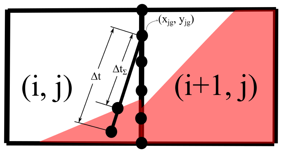
The shape of the interface is reconstructed by using the PLIC method, as shown in Figure 1, where C is the cell-averaged value of α . After the reconstruction of the interface, the space–time flux integral must be considered. Otherwise, the numerical method will blow up because of the inconsistency between VoF + PLIC and the compressible solver. The flux integral is computed according to Figure 2, where Δ t is the time step, and Δ t Σ is the time for the interface to arrive at the integral point.

2.3. Raindrop Generation

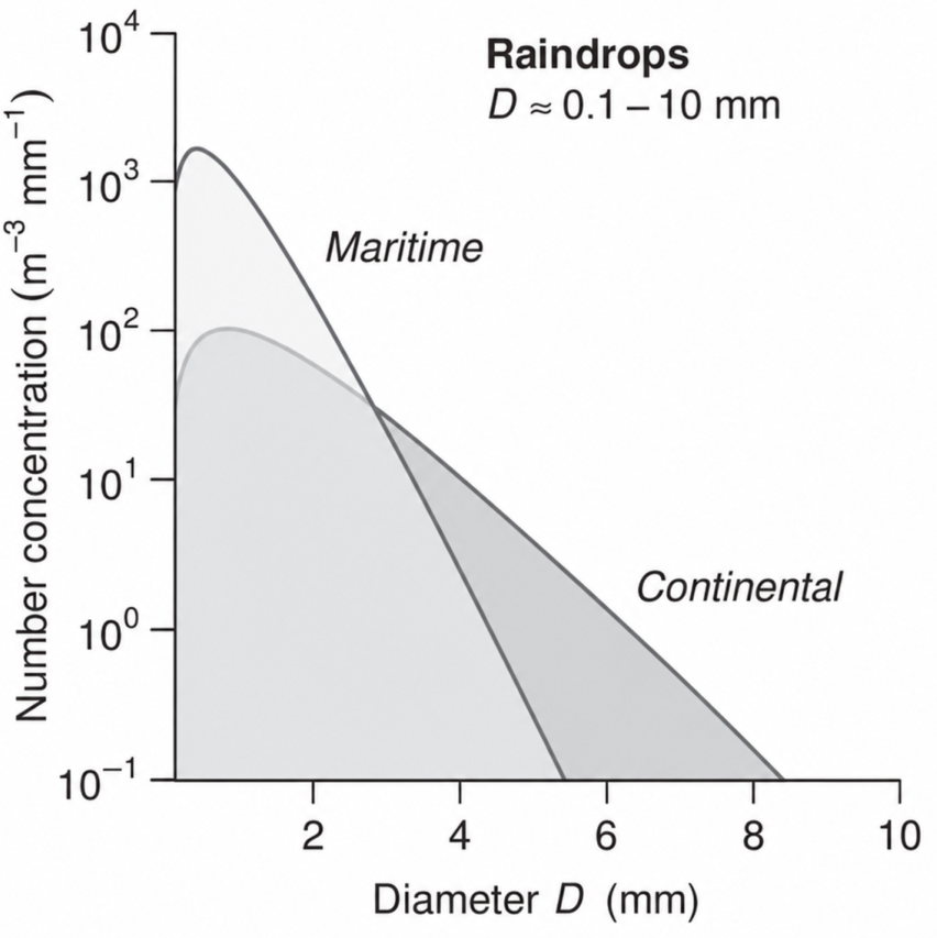
The methodology for generating statistically consistent raindrop fields consists of spectrum modeling, probabilistic diameter sampling, and spatial placement with collision control. A maritime empirical spectrum from Figure 3 is fitted with a fifth-order polynomial with respect to the diameter D:
log 10 N ( D ) = A 0 + A 1 D + A 2 D 2 + A 3 D 3 + A 4 D 4 + A 5 D 5 ,
where N ( D ) represents the number concentration function. For stochastic sampling, the spectrum is normalized to construct a probability density function,
PDF ( D ) = N ( D ) D min D max N ( D ) d D .
In Equation (18), D min is taken as 1.0 mm and D max as 5.0 mm in this work. When the distribution is truncated, the PDF is re-normalized to preserve statistical consistency.
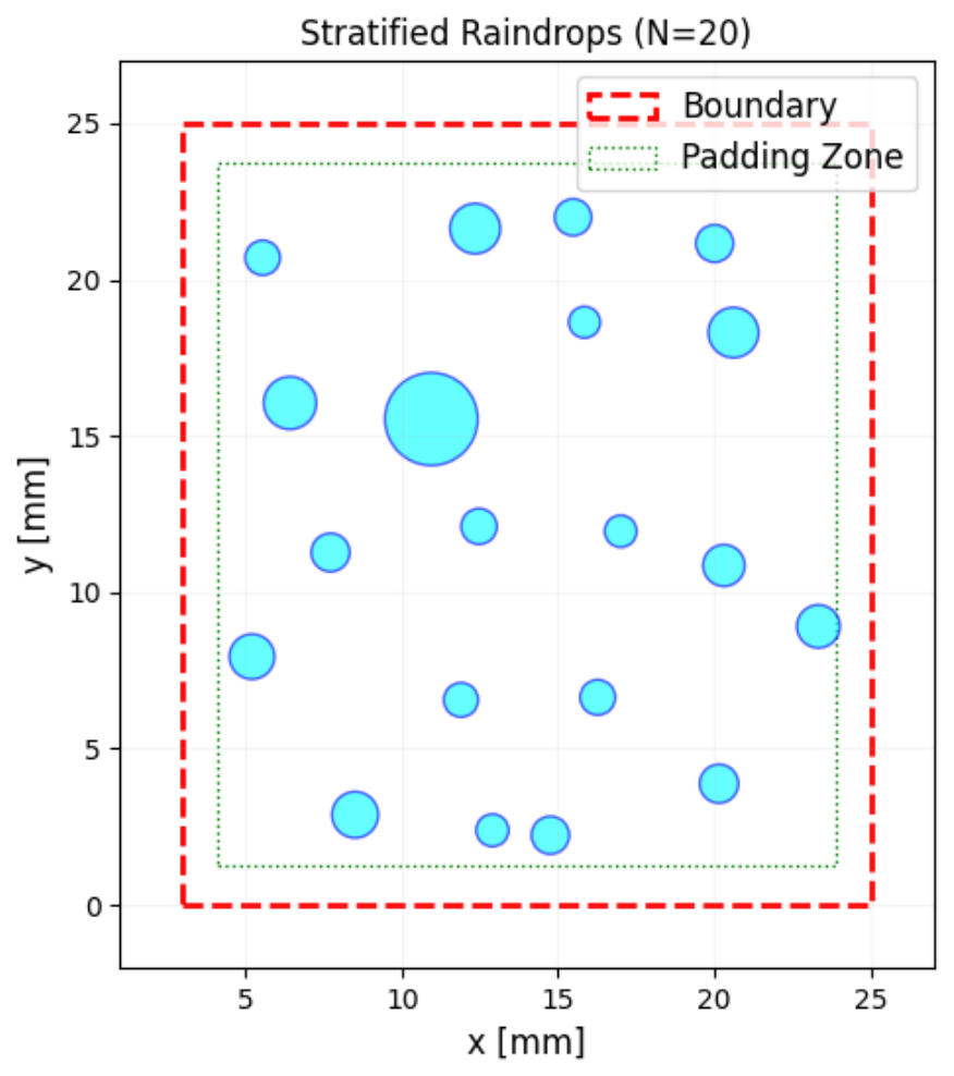
The diameters of raindrops are sampled using Monte Carlo method. The spatial distribution of raindrops is generated using a stratified sampling approach. The raindrops are generated within the domain of [ 3 mm x 25 mm ] , [ 0 y 25 mm ] . The domain is divided into quasi-uniform cells according to the number of raindrops, and one raindrop is assigned to each quasi-cell with a randomized offset from the cell center. This procedure improves spatial uniformity while maintaining randomness. Geometric overlap is prevented through a collision detection algorithm based on pairwise distance evaluation. The raindrop centers are restricted to the ‘padding zone’, ensuring full containment within the domain. The generation of 20 raindrops is given in Figure 4.

3. Results and Discussion

3.1. High-Pressure Water/Low-Pressure Air Shock Tube

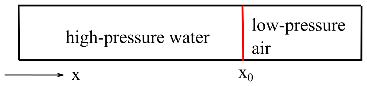
A shock tube with an initial interface between high-pressure liquid water and low-pressure air is set up over a 1.0 m domain, with the interface located at x 0 = 0.7 m (illustrated in Figure 5). The initial conditions, as described in [48], are as follows:
l i q u i d : z 1 = 1.0 ϵ c u t u = 0 p = 10 9 [ Pa ] ρ = 1000.0 [ kg / m 3 ] f o r x < x 0 , g a s : z 1 = ϵ c u t u = 0 p = 10 5 [ Pa ] ρ = 50.0 [ kg / m 3 ] f o r x x 0 ,
where x 0 = 0.7 m, and ϵ c u t = 1.0 × 10 10 . The heat capacity ratio of air is γ 1 = 1.4 , and for water γ 2 = 4.4 and p , 2 = 6.0 × 10 8 [ Pa ] .
The solutions were generated at t = 229 μs with a CFL number of 0.1 . Table 1 shows the relative error of total mass of liquid using three numerical schemes (first-order, Minmod, and van Leer) over increasing mesh resolutions N c e l l . Across all resolutions and limiters, the scheme conserves the liquid mass at 0.004–0.006% relative error. Among the three schemes, van Leer gives the smallest relative mass error.
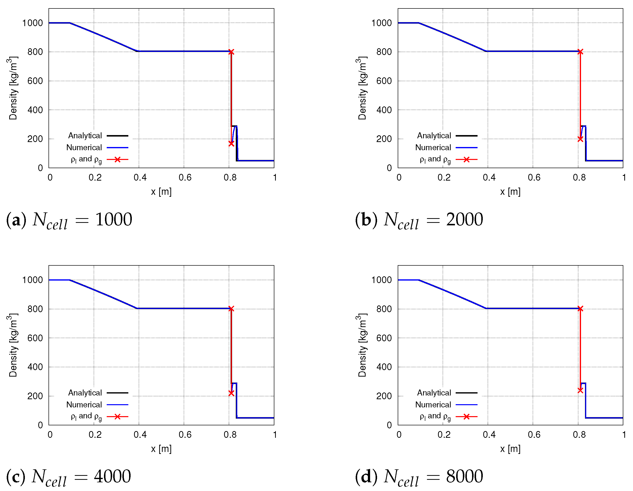
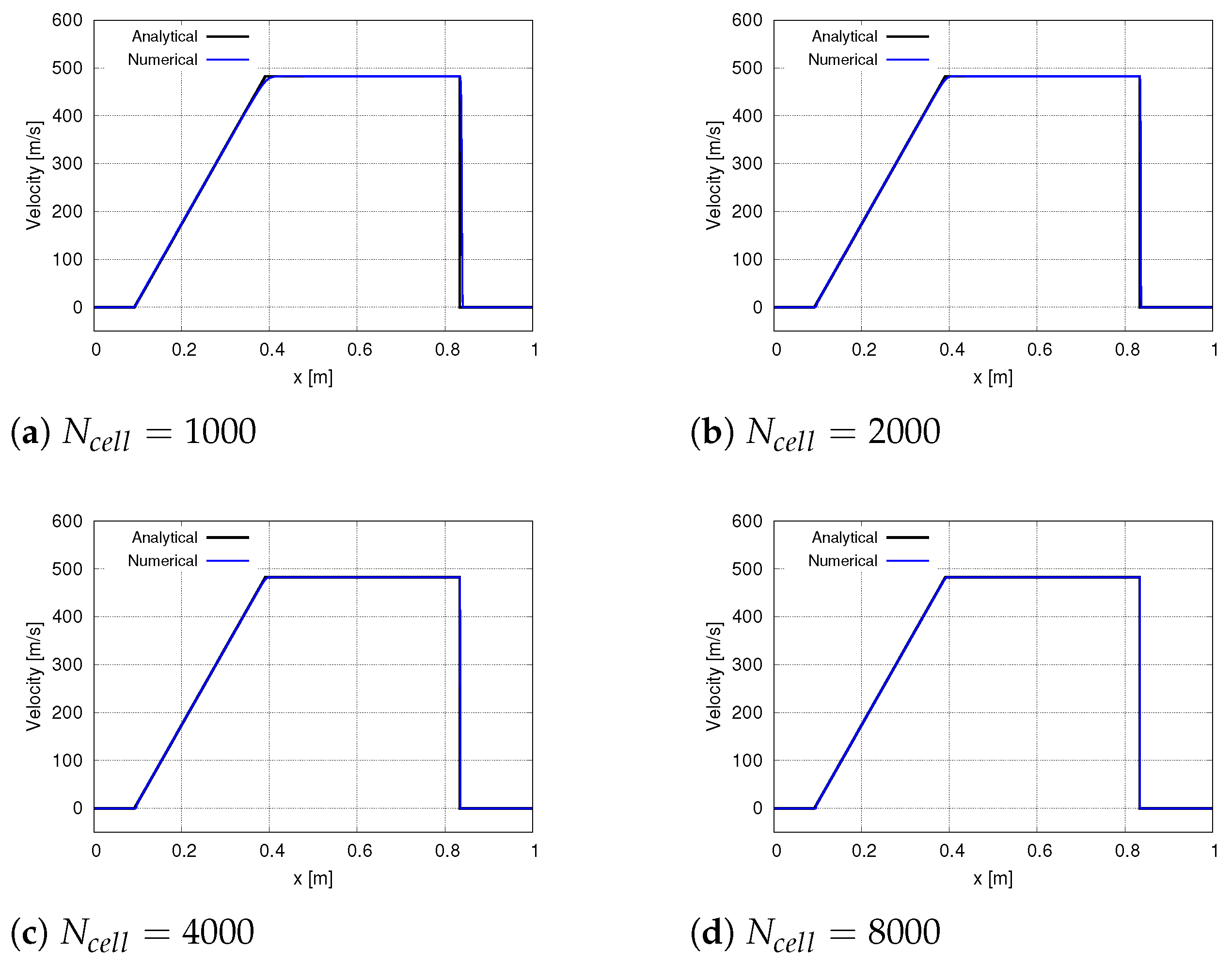
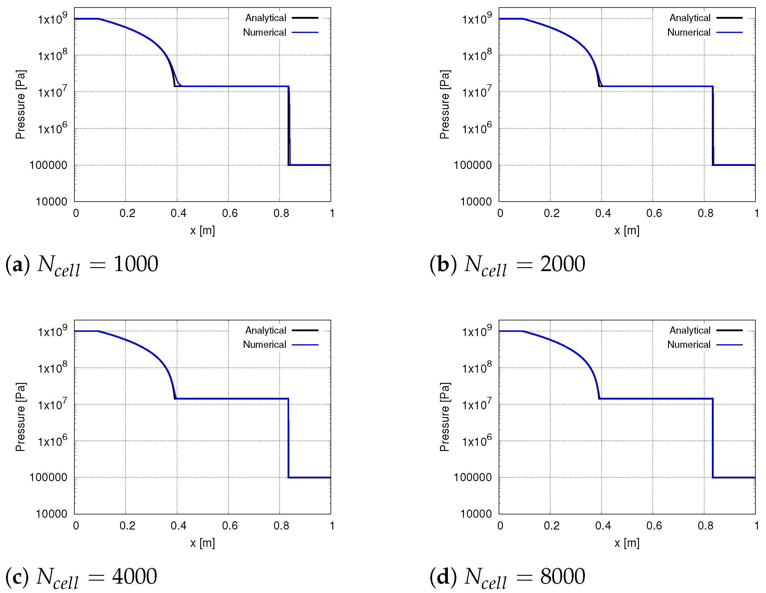
Figure 6, Figure 7, and Figure 8 show the comparison for density, velocity, and pressure, respectively, with the analytical solution using the van Leer limiter and four different N c e l l numbers: (a) 1000, (b) 2000, (c) 4000, and (d) 8000. This is a very challenging problem since the pressure ratio is 10,000, and the shock wave moving to the air phase is very weak relative to the expansion fan in the water. As can be seen from Figure 6a, there is a slight undershoot at the contact interface. However, the discontinuity is nearly as sharp as the analytical jump for N c e l l 4000 . Key shock and contact discontinuities are well captured across all resolutions. Red cross markers (liquid and gas densities) show that both phase densities remain consistent and match the analytical interface values. Increasing the mesh resolutions from N c e l l = 1000 to N c e l l = 8000 , the numerical solution converges cleanly to the analytical one.

3.2. Shock Wave in Air/Helium Bubble Interaction

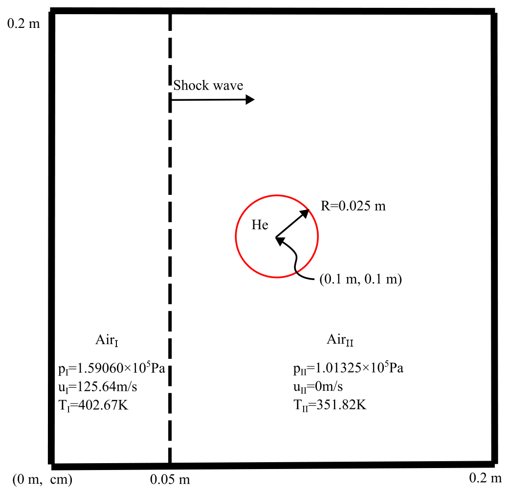
The initial conditions for the interaction between a shock wave in the air and a helium bubble are based on [37]. Originally investigated experimentally by Haas and Sturtevant [49], this setup serves as a benchmark for exploring the governing physics and validating numerical algorithms. The helium bubble, with a radius of 2.5 cm, is positioned 5.0 cm from the initial shock wave. Upstream of the shock wave, the pressure, velocity, and temperature are:
p I I = 1.01325 × 10 5 [ Pa ] , u I I = 0.0 [ m / s ] , T I I = 351.82 [ K ] .
Downstream of the shock wave, the pressure, velocity, and temperature are
p I = 1.59060 × 10 5 [ P a ] , u I = 125.65 [ m / s ] , T I = 402.67 [ K ] .
Figure 9 illustrates these initial conditions. The heat capacity ratio and the specific isochoric heat capacity of air are γ = 1.4 , and C v = 720 [ J / ( k g · K ) ] , respectively. For helium, these values are γ = 1.648 and C v = 2440 [ J / ( k g · K ) ] .
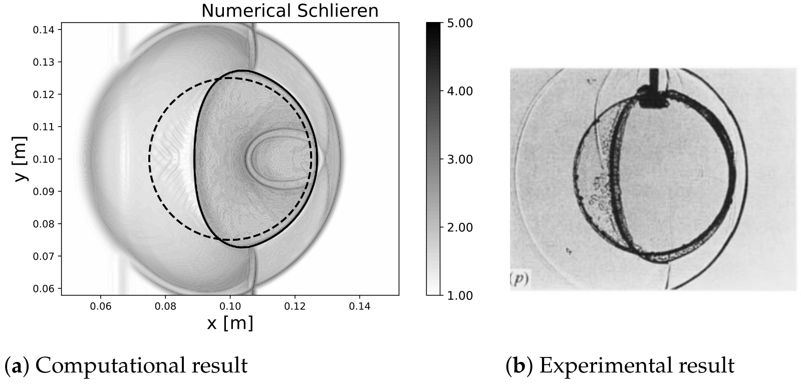
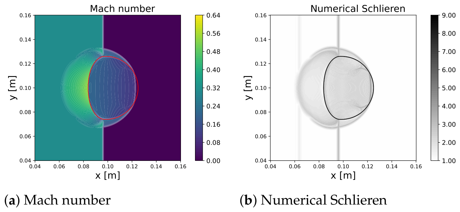
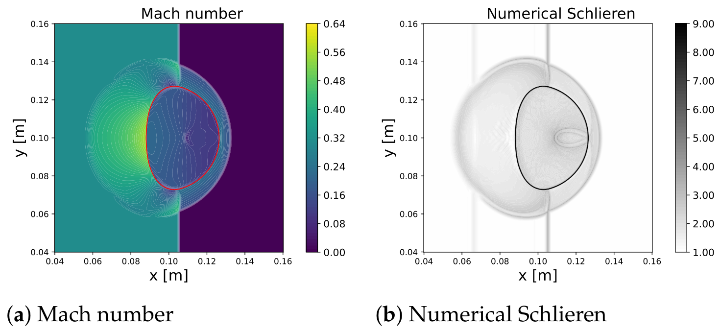
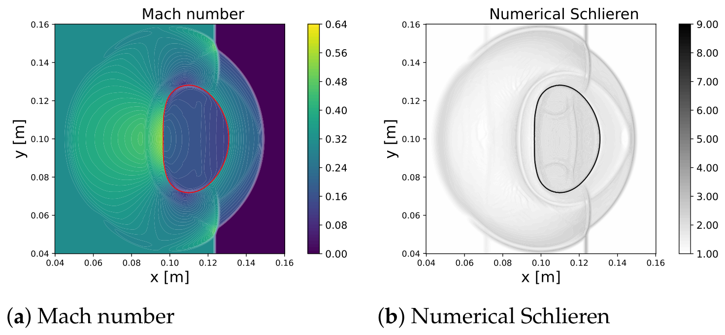
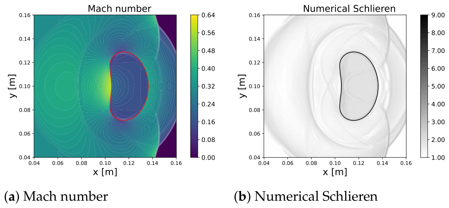
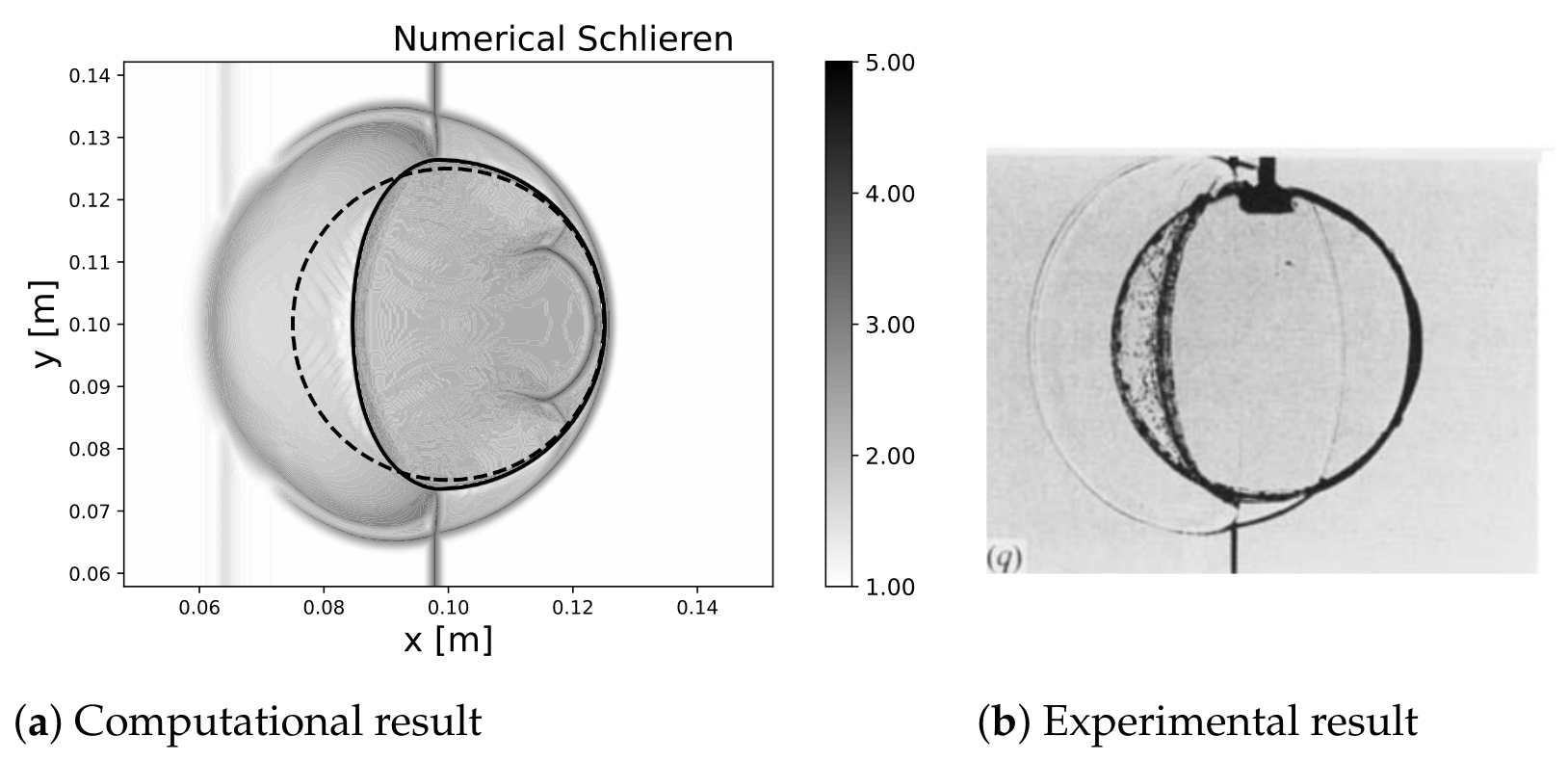
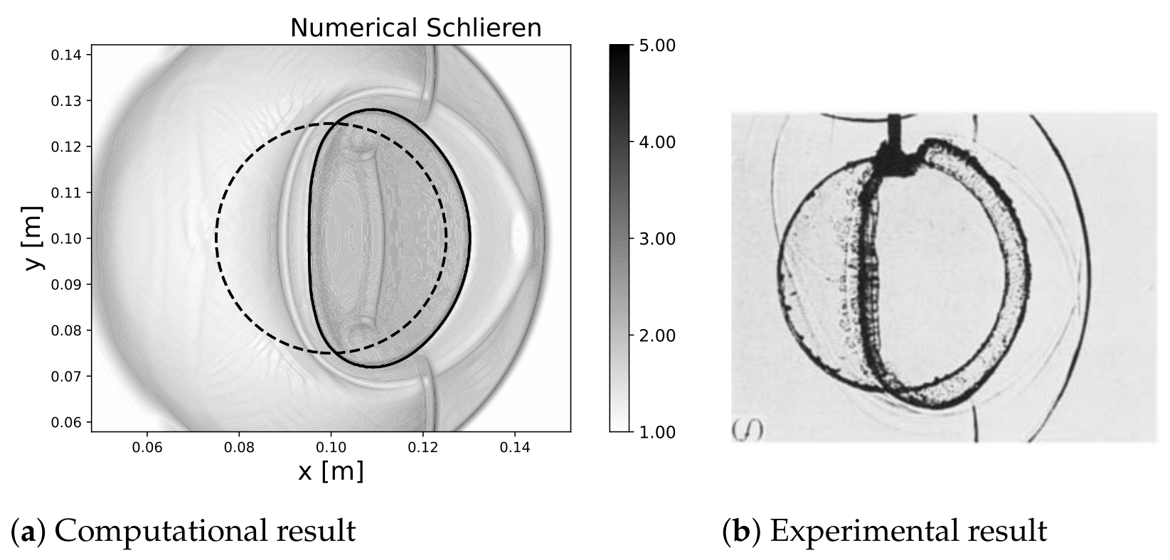
The computational domain spans 0.0 m x 0.2 m and 0.0 m y 0.2 m , with the helium bubble centered at ( x = 0.1 m , y = 0.1 m ) . The computational domain is discretized into 800 × 800 cells. The shock wave reaches the helium bubble at t 0 = 52 μs. Figure 10a,b display the Mach number contours and numerical Schileren images at t = 100 μs, while Figure 11a,b show these at t = 120 μs. Mach number contours and Schlieren images at t = 160 μs and t = 200 μs are provided in Figure 12 and Figure 13, respectively. In this test case, C represents the volume fraction of helium. Comparisons between the numerical results and experimental data from [49], presented in Figure 14, Figure 15 and Figure 16, show strong agreement. The computational (on the left) and the experimental (on the right) results both illustrate the deformation of the helium bubble over time due to the shock wave interaction. The initial bubble shape (dashed line) becomes increasingly distorted (solid line) as the shock wave passes through. The numerical Schlieren results closely match the experimental observations, capturing the deformation and wave interactions effectively. This agreement confirms the model’s capability in accurately representing the key physical mechanisms and the temporal evolution of the helium bubble’s shape. As time progresses from t t 0 = 52 μs to t t 0 = 102 μs, the bubble undergoes significant elongation and distortion. The numerical model accurately replicates these deformations and the accompanying wave structures, demonstrating strong quantitative agreement and validating the effectiveness of the numerical method in depicting shock-bubble dynamics.

3.3. Mach 1.36 Shock Wave Interacting with One Raindrop

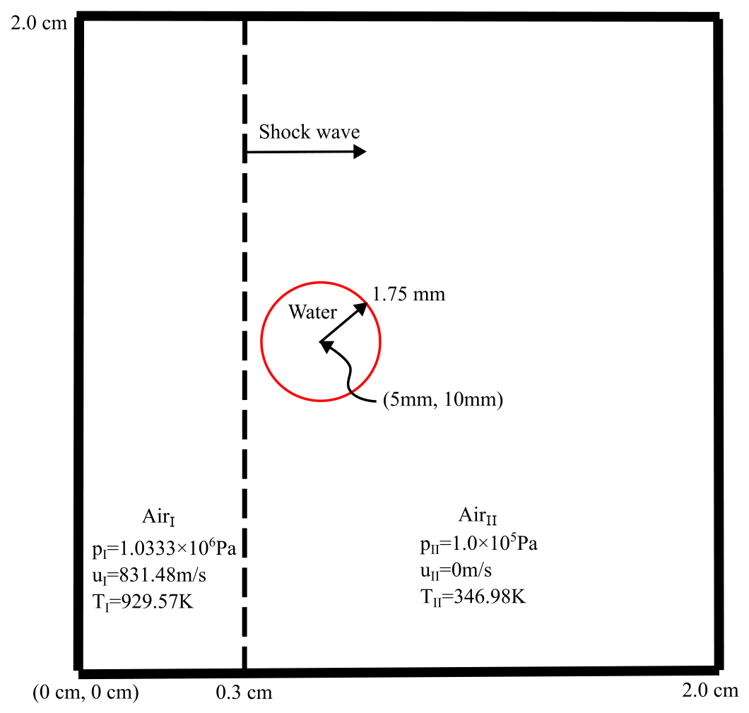
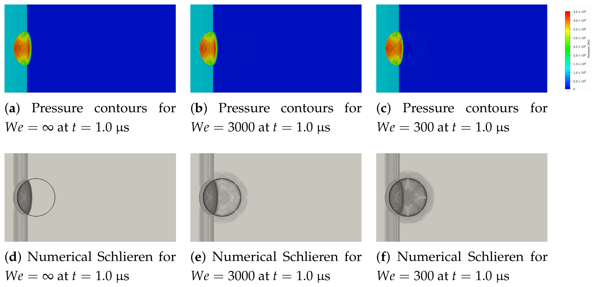
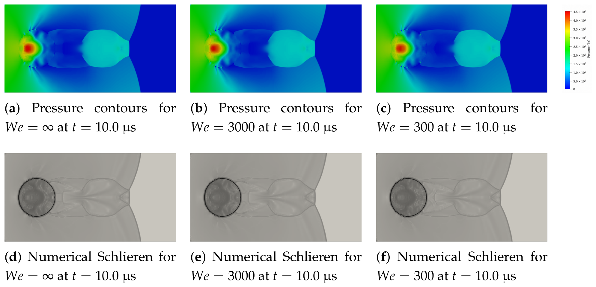
This test case investigates the interaction between a strong planar shock wave and a liquid raindrop to assess whether surface tension effects can be considered negligible under high compressible flow conditions. The initial condition is given in Figure 17 with a coming shock wave of M a c h = 1.36 . Three conditions are compared by varying the Weber number: W e = , W e = 3000 , and W e = 300 , allowing evaluation of whether surface tension can be neglected without significantly affecting raindrop deformation dynamics and overall flow evolution.
Figure 18 and Figure 19 compare the pressure contours and numerical Schlieren fields at early ( t = 1.0 μs) and later ( t = 10.0 μs) times under different Weber numbers ( W e = , W e = 3000 , and W e = 300 ). At both instants, the overall shock structure, wave patterns, and pressure peak remain nearly identical across all Weber numbers considered. In particular, the incident shock strength, its reflection at the raindrop interface, and the downstream wake topology show negligible sensitivity to surface tension. Minor differences are limited to small-scale interfacial smoothing near the raindrop boundary, which does not affect the global shock dynamics or pressure distribution. These observations indicate that, for the strong shock regime examined in this work, the characteristic inertial and compressibility effects dominate the flow evolution, while capillary forces play a secondary role. Consequently, surface tension has a negligible influence on both the early shock impact process and the subsequent wave–raindrop interaction, justifying its omission in the governing equations for the present shock-dominated flow regime.
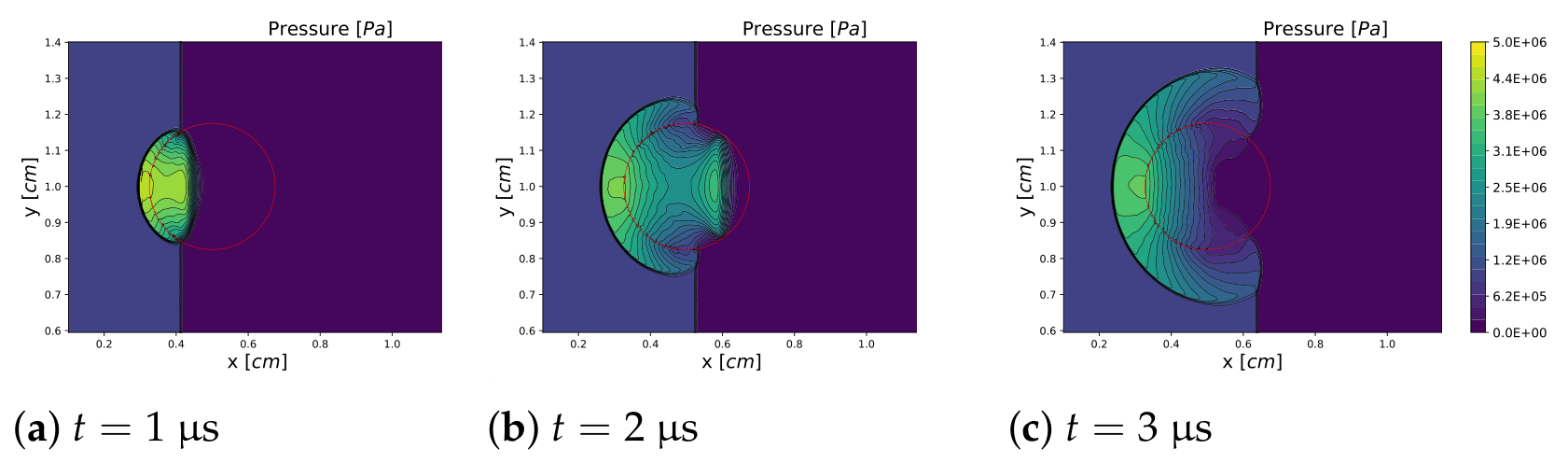
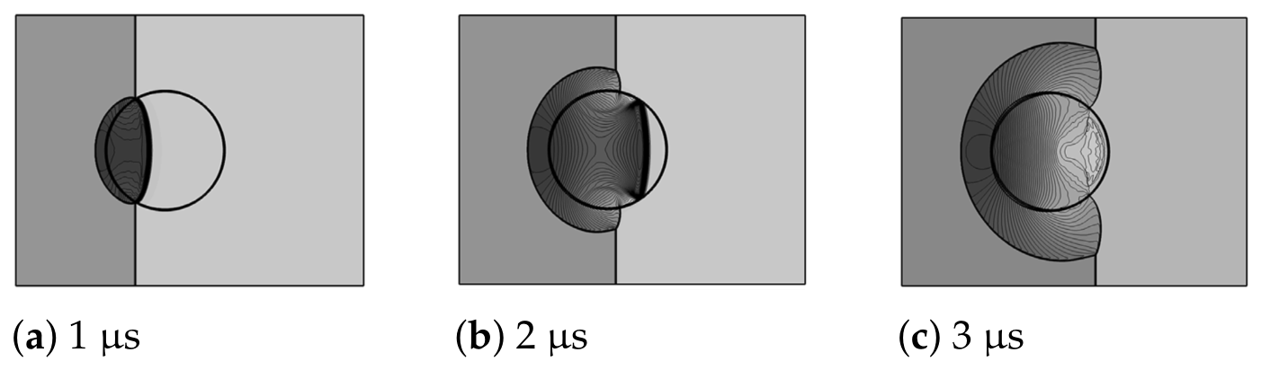
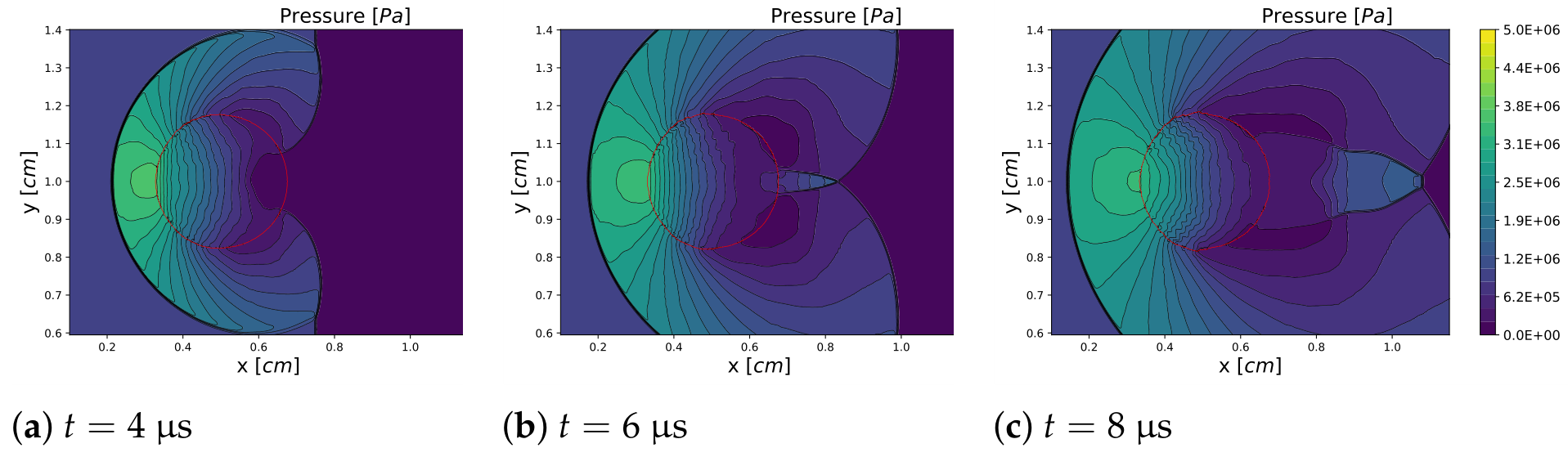
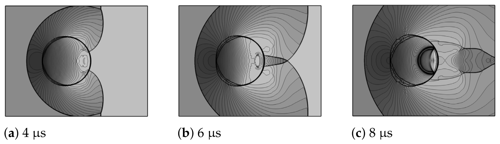
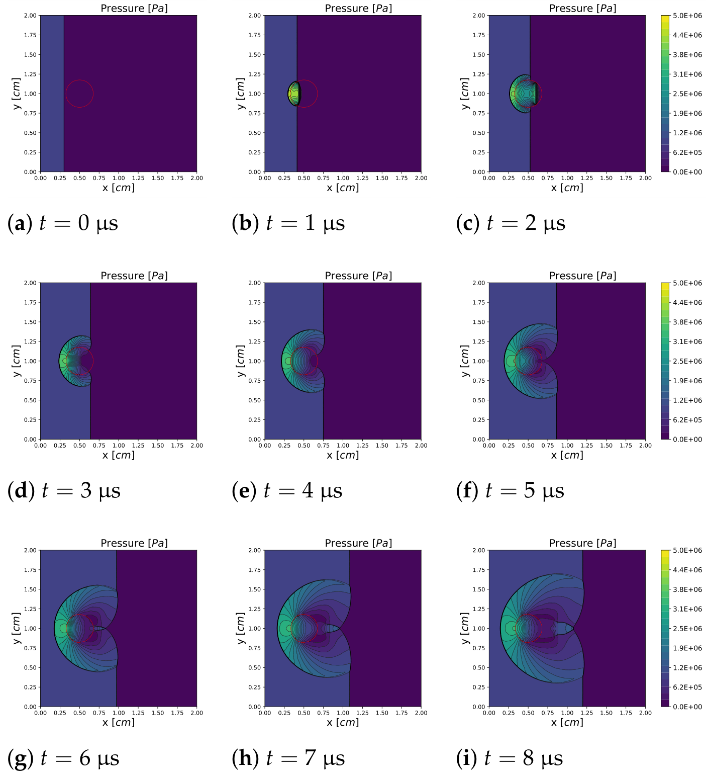
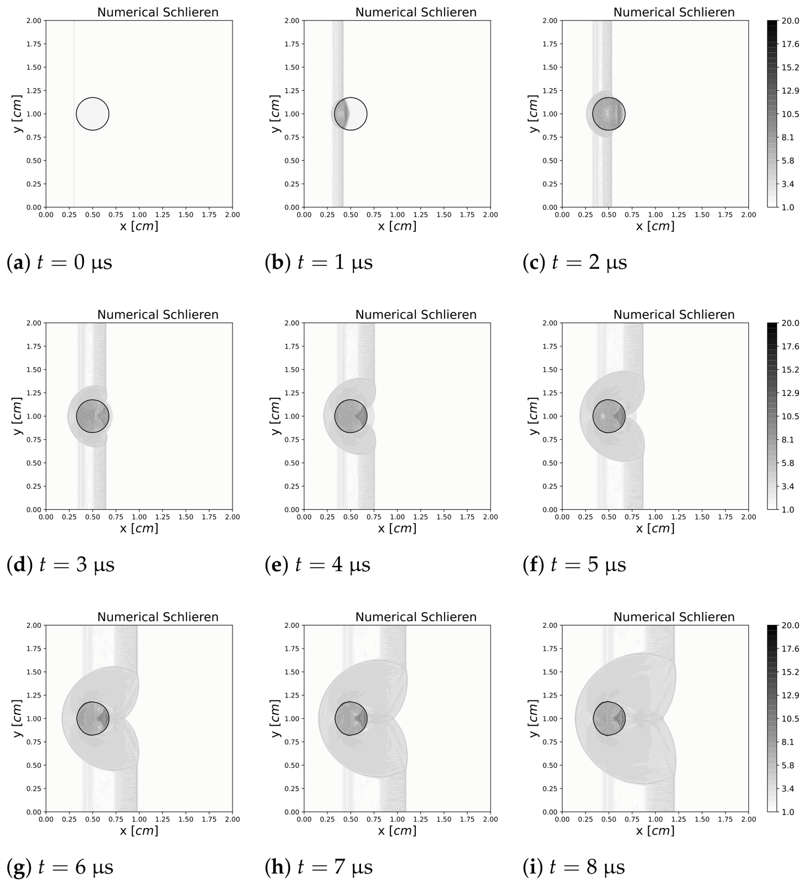
Figure 20 displays the pressure contours at 1 μs, 2 μs, and 3 μs, with the interface marked by a red line, while the corresponding results from [50] are shown in Figure 21. Similarly, the computed pressure contours at 4 μs, 6 μs, and 8 μs are presented in Figure 22, with the results from [50] displayed in Figure 23. As time progresses (from 1 μs to 8 μs), the shock wave dynamically interacts with the droplet. From 1 μs (Figure 20a and Figure 21a) to 3 μs (Figure 20c and Figure 21c), the shock wave deforms as it interacts and travels through the droplet. At later times ( 4 μs, 6 μs, 8 μs), the pressure contours indicate further deformation of the droplet. The numerical results (Figure 20 and Figure 22) align well with the results from the literature (Chang and Liou [50]), demonstrating that the model’s ability to produce expected results for droplet behavior under shock wave influence. Moreover, the present method enhances the accuracy of the sharp-interface representation, as evident in Figure 22c compared to Figure 23c. The progression of pressure contours across the entire computational domain is shown in Figure 24, while the evolution of the numerical Schlieren is presented in Figure 25.
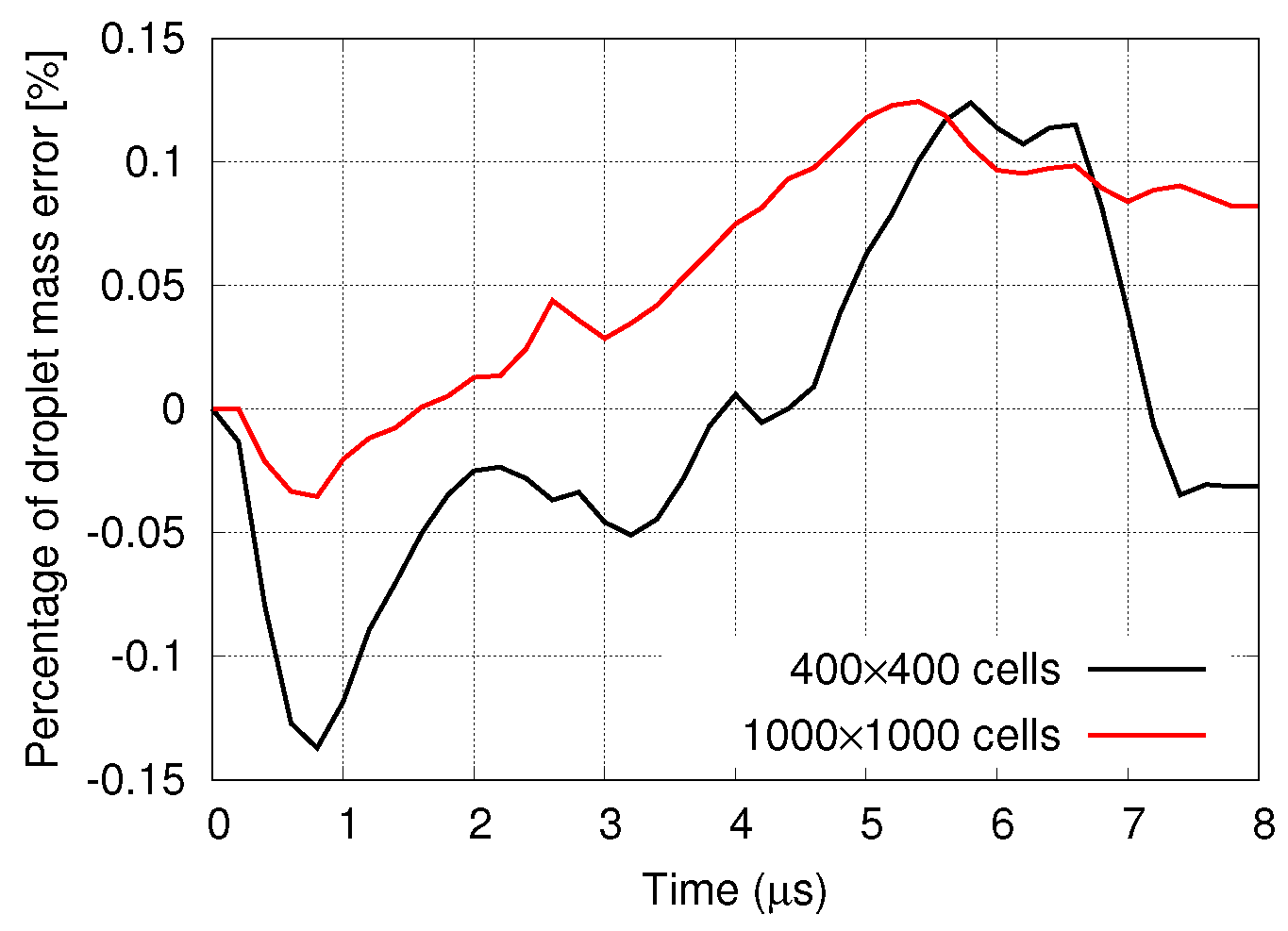
Figure 26 presents the total mass error of the droplet over time during the shock-wave and droplet interaction, comparing results for two grid resolutions: 400 × 400 cells (black line) and 1000 × 1000 cells (red line). Both simulations show mass errors within 0.15 % , indicating stable behavior of the droplet’s total mass.

3.4. Mach 1.73 Shock Wave Interacting with Two Raindrops

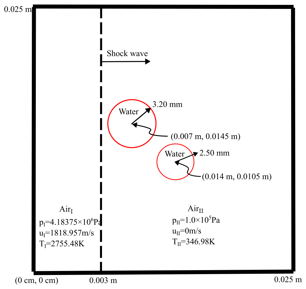
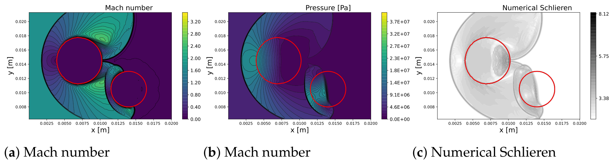
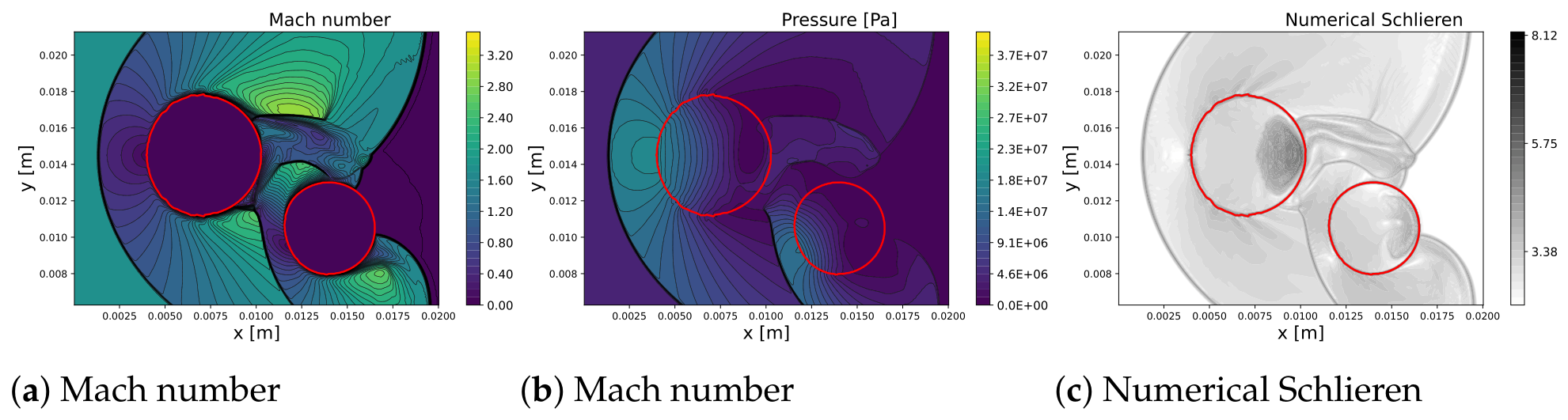
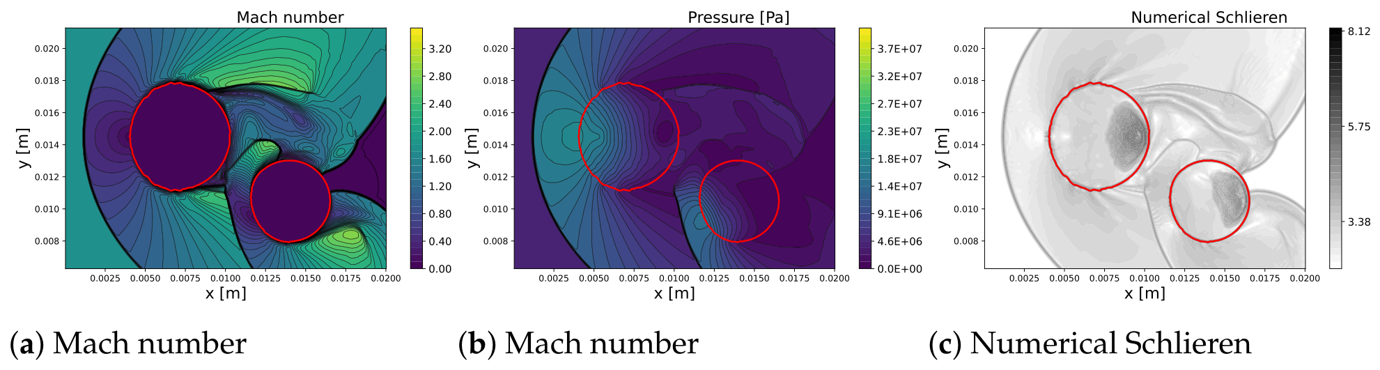
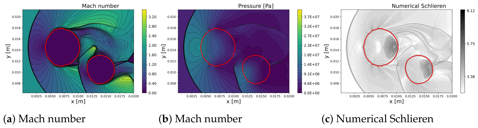
Figure 27 illustrates the initial configuration for the interaction of a planar shock wave with two water raindrops in air. A planar shock wave of M a c h = 1.73 propagates in x-direction, corresponding to a nominal supersonic flow. Two initially stationary, circular water raindrops are embedded downstream of the shock, with radii of 3.20 mm and 2.50 mm. This configuration enables the investigation of shock interaction with two raindrops of different sizes, including the effects of wave transmission, reflection, and raindrop–raindrop interaction in a shock-dominated flow regime.
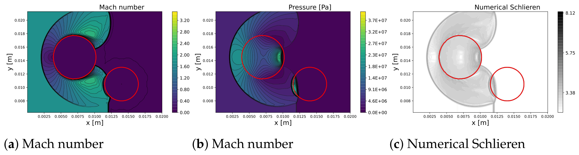
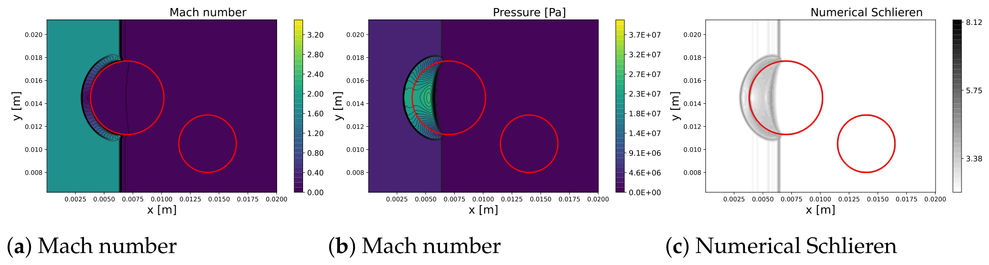
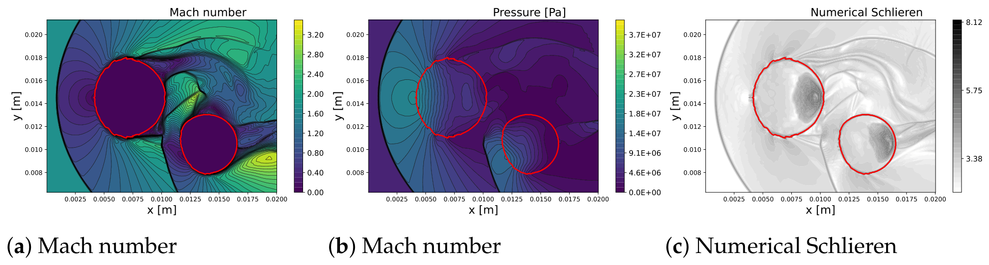
Figure 28, Figure 29, Figure 30, Figure 31, Figure 32, Figure 33, Figure 34, Figure 35 and Figure 36 show the temporal evolution of Mach number, pressure contours, and numerical Schlieren. Upon impact with the upstream raindrop (Figure 28), a strong pressure augmentation forms at the windward stagnation point, accompanied by a sharp Mach number reduction. The incident shock is reflected and diffracted around the raindrop, generating curved shock fronts and lateral expansion waves along the raindrop surface. As the interaction develops (Figure 29 and Figure 30), the transmitted shock subsequently impinges on the downstream raindrop, leading to secondary pressure amplification and additional reflected and diffracted wave structures. At later times (Figure 31, Figure 32, Figure 33, Figure 34, Figure 35 and Figure 36), multiple shock and expansion waves interact between the two raindrops. Both raindrops undergo progressive deformation driven primarily by shock-induced pressure gradients, with the upstream raindrop experiencing stronger flattening and lateral stretching, while the downstream raindrop deforms under the combined effects of transmitted shocks and wake-induced flow structures.

3.5. Mach 1.73 Shock Wave Interacting with Twenty Raindrops

To study the interference of multiple raindrops, the two raindrops in Section 3.4 are replaced with twenty raindrops. The methodology for generating statistically consistent raindrop fields consists of spectrum modeling, probabilistic diameter sampling, and spatial placement with collision control. A maritime empirical spectrum from Figure 3 is fitted with a fifth-order polynomial with respect to the diameter D:
log 10 N ( D ) = 3.0697 + 0.6732 D 1.2068 D 2 + 0.4502 D 3 0.0792 D 4 + 0.0052 D 5 .
Figure 37 and Figure 38 present the temporal evolution of the Mach number and pressure fields. At early times (t = 1.0–3.0 μs), the incident planar shock is progressively distorted as it encounters individual droplets. As the shock wave penetrates deeper into the droplets, multiple reflected shocks and expansion waves emerge, leading to pronounced wave curvature and strong non-uniformity in both Mach number and pressure. The interaction between neighboring raindrops results in wave interference and cumulative pressure amplification. At later times (t = 6.0–12.0 μs), the flow field is dominated by a complex network of interacting shocks and expansion fans. Despite the strong wave–interface interactions and significant droplet deformation, the interfaces remain sharply resolved without numerical smearing. These results highlight the importance of accounting for multi-raindrop collective effects and demonstrate the capability of the proposed sharp-interface flux-integral method to robustly capture complex shock–raindrop interactions under realistic conditions.

4. Conclusions

A density-based solution strategy and geometric VoF + PLIC method are combined to study the interaction between a shock wave and multiple raindrops. A space–time flux-integral method is brought about to make the density-based method consistent with VoF + PLIC.
The comparison between analytical solution, experimental results and numerical results is made for the gas–liquid shock wave problem and shock wave interaction with a helium bubble. The simulations of shock waves and raindrops have provided insights into wave structures and wake flow.
The principal contribution of this work is the development of a density-based sharp-interface framework for strongly compressible gas–liquid flows, where both phases are treated as compressible media and coupled through a geometric VoF + PLIC interface representation. Instead of using Tait equations of state, stiffened gas equations of state are used for both phases to account for the strong compressible effects. Unlike conventional VoF approaches developed primarily for incompressible or weakly compressible applications, the proposed method is designed for shock-dominated multiphase flows. Furthermore, the simulations provide new insights into shock interactions with multiple raindrops, highlighting the importance of wave interference and droplet-group effects.
Future work will focus on the detailed analysis of the bow shock wave location, the displacement of individual raindrops, and cavitation phenomena within the droplets.

Author Contributions

Conceptualization, L.L.; Methodology, L.L. and Z.Y.; Validation, L.L.; Formal analysis, L.L.; Investigation, L.L.; Data curation, Z.Y. and L.T.; Writing—original draft, L.L.; Writing—review & editing, J.L., J.Y. and L.T.; Project administration, L.L.; Funding acquisition, X.Y. All authors have read and agreed to the published version of the manuscript.

Funding

This work was supported by the National Key Research and Development Program of China (Grant No. 2024YFB3310400) and the National Natural Science Foundation of China (Grants No. U24A2007, and No. 12421002).

Institutional Review Board Statement

Not applicable.

Informed Consent Statement

Not applicable.

Data Availability Statement

Data will be made available upon reasonable request.

Conflicts of Interest

The authors declare no conflicts of interest.

References

  1. Meng, J.; Colonius, T. Numerical simulation of the aerobreakup of a water droplet. J. Fluid Mech. 2018, 835, 1108–1135. [Google Scholar] [CrossRef] [Scilit]
  2. Poplavski, S.; Minakov, A.; Shebeleva, A.; Boiko, V. On the interaction of water droplet with a shock wave: Experiment and numerical simulation. Int. J. Multiph. Flow 2020, 127, 103273. [Google Scholar] [CrossRef] [Scilit]
  3. Virot, F.; Tymen, G.; Hébert, D.; Rullier, J.L.; Lescoute, E. Experimental investigation of the interaction between a water droplet and a shock wave above Mach 4. Shock Waves 2023, 33, 369–383. [Google Scholar] [CrossRef] [Scilit]
  4. Forehand, R.; Nguyen, K.; Anderson, C.; Shannon, R.; Grace, S.; Kinzel, M. A numerical assessment of shock–droplet interaction modeling including cavitation. Phys. Fluids 2023, 35, 023315. [Google Scholar] [CrossRef] [Scilit]
  5. Wang, Z.; Hopfes, T.; Giglmaier, M.; Adams, N. Effect of Mach number on droplet aerobreakup in shear stripping regime. Exp. Fluids 2020, 61, 193. [Google Scholar] [CrossRef] [Scilit] [PubMed]
  6. Chandra, N.; Sharma, S.; Basu, S.; Kumar, A. Shock-induced aerobreakup of a polymeric droplet. J. Fluid Mech. 2023, 965, A1. [Google Scholar] [CrossRef] [Scilit]
  7. Schroeder, S.; Salauddin, S.; Morales, A.; Moran, M.; Hytovick, R.; Rigney, E.; Ahmed, K. Deformation and aerobreakup of RP-2 droplets from hypersonic shock waves. Proc. Combust. Inst. 2024, 40, 105338. [Google Scholar] [CrossRef] [Scilit]
  8. Zhang, Y.; Dong, R.; Shi, H.; Liu, J. Experimental Investigations on the Deformation and Breakup of Hundred-Micron Droplet Driven by Shock Wave. Appl. Sci. 2023, 13, 5555. [Google Scholar] [CrossRef] [Scilit]
  9. Li, L.; Löhner, R.; Pandare, A.K.; Luo, H. A vertex-centered finite volume method with interface sharpening technique for compressible two-phase flows. J. Comput. Phys. 2022, 460, 111194. [Google Scholar]
  10. Zhu, W.; Zheng, H.; Zhao, N. Numerical investigations on the deformation and breakup of an n-Decane droplet induced by shock wave. Phys. Fluids 2022, 34, 063306. [Google Scholar] [CrossRef] [Scilit]
  11. Biasiori-Poulanges, L.; Schmidmayer, K. A phenomenological analysis of droplet shock-induced cavitation using a multiphase modeling approach. Phys. Fluids 2022, 35, 013312. [Google Scholar] [CrossRef] [Scilit]
  12. Huang, X.; Lin, Z. Study of the mechanism of shock-induced and detonation-induced droplet breakup based on hybrid solvers. Phys. Fluids 2024, 36, 086102. [Google Scholar] [CrossRef] [Scilit]
  13. Xu, S.; Jin, X.; Fan, W.; Wen, H.; Wang, B. Numerical investigation on the interaction characteristics between the gaseous detonation wave and the water droplet. Combust. Flame 2024, 269, 113713. [Google Scholar] [CrossRef] [Scilit]
  14. Xiong, T.; Shao, C.; Luo, K. Exploration of shock–droplet interaction based on high-fidelity simulation and improved theoretical model. J. Fluid Mech. 2024, 988, A46. [Google Scholar] [CrossRef] [Scilit]
  15. Ullman, M.; Bielawski, R.; Raman, V. Timescales and statistics of shock-induced droplet breakup. Phys. Rev. Fluids 2025, 10, 124301. [Google Scholar] [CrossRef] [Scilit]
  16. Song, J.; Long, T.; Pan, S. Three-dimensional numerical simulations of phase change effects on shock-droplet interactions. Phys. Fluids 2025, 37, 033358. [Google Scholar] [CrossRef] [Scilit]
  17. Chen, H.; Jin, X.; Wang, W.; Xu, S.; Wang, B. Investigation on the dynamic characteristics of a droplet subjected to a divergent shock wave. Phys. Fluids 2025, 37, 086159. [Google Scholar] [CrossRef] [Scilit]
  18. Song, J.; Zhou, W.; Shang, W.; Li, J.; Zhang, Q.; Yin, X.; Liu, J.; Liu, S. Numerical simulation of the effects of spraying parameters on the bow shock wave and atomized droplets deposition. Mater. Chem. Phys. 2025, 341, 130919. [Google Scholar] [CrossRef] [Scilit]
  19. Verma, M.; Udaykumar, H. Effect of counter-propagating shock waves on the aerodynamic breakup of a liquid droplet. Int. J. Multiph. Flow 2026, 198, 105659. [Google Scholar] [CrossRef] [Scilit]
  20. Shukla, R.K.; Pantano, C.; Freund, J.B. An interface capturing method for the simulation of multi-phase compressible flows. J. Comput. Phys. 2010, 229, 7411–7439. [Google Scholar] [CrossRef] [Scilit]
  21. Sussman, M.; Smith, K.M.; Hussaini, M.Y.; Ohta, M.; Zhi-Wei, R. A sharp interface method for incompressible two-phase flows. J. Comput. Phys. 2007, 221, 469–505. [Google Scholar] [CrossRef] [Scilit]
  22. Mulder, W.; Osher, S.; Sethian, J.A. Computing interface motion in compressible gas dynamics. J. Comput. Phys. 1992, 100, 209–228. [Google Scholar] [CrossRef] [Scilit]
  23. Karni, S. Multicomponent flow calculations by a consistent primitive algorithm. J. Comput. Phys. 1994, 112, 31–43. [Google Scholar] [CrossRef] [Scilit]
  24. Karni, S. Hybrid multifluid algorithms. SIAM J. Sci. Comput. 1996, 17, 1019–1039. [Google Scholar] [CrossRef] [Scilit]
  25. Hirt, C.W.; Nichols, B.D. Volume of fluid (VOF) method for the dynamics of free boundaries. J. Comput. Phys. 1981, 39, 201–225. [Google Scholar] [CrossRef] [Scilit]
  26. Zhang, B.; Boyd, B.; Ling, Y. Direct numerical simulation of compressible interfacial multiphase flows using a mass–momentum–energy consistent volume-of-fluid method. Comput. Fluids 2022, 236, 105267. [Google Scholar]
  27. Sementilli, M.L.; McGurn, M.T.; Chen, J. A scalable compressible Volume of Fluid solver using a Stratified Flow model. Int. J. Numer. Methods Fluids 2022, 95, 777–795. [Google Scholar]
  28. Ye, Z.; Estebe, C.; Liu, Y.; Vahab, M.; Huang, Z.; Sussman, M.; Moradikazerouni, A.; Shoele, K.; Lian, Y.; Ohta, M.; et al. An Improved Coupled Level Set and Continuous Moment-of-Fluid Method for Simulating Multiphase Flows with Phase Change. Commun. Appl. Math. Comput. 2023, 6, 1034–1069. [Google Scholar] [CrossRef] [Scilit]
  29. Shin, S.; Lee, W.I. Finite element analysis of incompressible viscous flow with moving free surface by selective volume of fluid method. Int. J. Heat Fluid Flow 2000, 21, 197–206. [Google Scholar] [CrossRef] [Scilit]
  30. Son, G. Efficient implementation of a coupled level-set and volume-of-fluid method for three-dimensional incompressible two-phase flows. Numer. Heat Transf. Part B Fundam. 2003, 43, 549–565. [Google Scholar]
  31. Park, I.R.; Kim, K.S.; Kim, J.; Van, S.H. A volume-of-fluid method for incompressible free surface flows. Int. J. Numer. Methods Fluids 2009, 61, 1331–1362. [Google Scholar]
  32. Sun, D.L.; Tao, W.Q. A coupled volume-of-fluid and level set (VOSET) method for computing incompressible two-phase flows. Int. J. Heat Mass Transf. 2010, 53, 645–655. [Google Scholar]
  33. Ling, K.; Li, Z.H.; Sun, D.L.; He, Y.L.; Tao, W.Q. A three-dimensional volume of fluid & level set (VOSET) method for incompressible two-phase flow. Comput. Fluids 2015, 118, 293–304. [Google Scholar]
  34. Nguyen, V.T.; Park, W.G. A volume-of-fluid (VOF) interface-sharpening method for two-phase incompressible flows. Comput. Fluids 2017, 152, 104–119. [Google Scholar]
  35. Arrufat, T.; Crialesi-Esposito, M.; Fuster, D.; Ling, Y.; Malan, L.; Pal, S.; Scardovelli, R.; Tryggvason, G.; Zaleski, S. A mass-momentum consistent, volume-of-fluid method for incompressible flow on staggered grids. Comput. Fluids 2021, 215, 104785. [Google Scholar]
  36. Bo, W.; Grove, J.W. A volume of fluid method based ghost fluid method for compressible multi-fluid flows. Comput. Fluids 2014, 90, 113–122. [Google Scholar] [CrossRef] [Scilit]
  37. Denner, F.; Xiao, C.N.; van Wachem, B.G. Pressure-based algorithm for compressible interfacial flows with acoustically-conservative interface discretisation. J. Comput. Phys. 2018, 367, 192–234. [Google Scholar]
  38. Duret, B.; Canu, R.; Reveillon, J.; Demoulin, F.X. A pressure based method for vaporizing compressible two-phase flows with interface capturing approach. Int. J. Multiph. Flow 2018, 108, 42–50. [Google Scholar] [CrossRef] [Scilit]
  39. Shen, Y.; Ren, Y.; Ding, H. A 3D conservative sharp interface method for simulation of compressible two-phase flows. J. Comput. Phys. 2020, 403, 109107. [Google Scholar] [CrossRef] [Scilit]
  40. Kuhn, M.B.; Desjardins, O. An all-Mach, low-dissipation strategy for simulating multiphase flows. J. Comput. Phys. 2021, 445, 110602. [Google Scholar]
  41. Nguyen, V.T.; Phan, T.H.; Duy, T.N.; Kim, D.H.; Park, W.G. Modeling of the bubble collapse with water jets and pressure loads using a geometrical volume of fluid based simulation method. Int. J. Multiph. Flow 2022, 152, 104103. [Google Scholar] [CrossRef] [Scilit]
  42. Wang, Z.; Sun, T.; Yang, Z.; Zhu, G.; Shi, H. Interactions between Two Deformable Droplets in Tandem Fixed in a Gas Flow Field of a Gas Well. Appl. Sci. 2021, 11, 11220. [Google Scholar] [CrossRef] [Scilit]
  43. Tripathi, M.; Ganti, H.; Khare, P. Interactions Between Shock Waves and Liquid Droplet Clusters: Interfacial Physics. J. Fluids Eng. 2022, 144, 101401. [Google Scholar] [CrossRef] [Scilit]
  44. Xu, Y.; Zhang, H. Interactions between a propagating detonation wave and circular water cloud in hydrogen/air mixture. Combust. Flame 2022, 245, 112369. [Google Scholar] [CrossRef] [Scilit]
  45. Allaire, G.; Clerc, S.; Kokh, S. A five-equation model for the simulation of interfaces between compressible fluids. J. Comput. Phys. 2002, 181, 577–616. [Google Scholar] [CrossRef] [Scilit]
  46. Saurel, R.; Metayer, O.L.; Massoni, J.; Gavrilyuk, S. Shock jump relations for multiphase mixtures with stiff mechanical properties. Shock Waves 2007, 16, 209–232. [Google Scholar]
  47. Tenório, R.S.; Moraes, M.C.D.S.; Sauvageot, H. Raindrop size distribution and radar parameters in coastal tropical rain systems of northeastern Brazil. J. Appl. Meteorol. Climatol. 2012, 51, 1960–1970. [Google Scholar] [CrossRef] [Scilit]
  48. Yeom, G.S.; Chang, K.S. A modified HLLC-type Riemann solver for the compressible six-equation two-fluid model. Comput. Fluids 2013, 76, 86–104. [Google Scholar]
  49. Haas, J.F.; Sturtevant, B. Interaction of weak shock waves with cylindrical and spherical gas inhomogeneities. J. Fluid Mech. 1987, 181, 41–76. [Google Scholar] [CrossRef] [Scilit]
  50. Chang, C.; Liou, M.S. A robust and accurate approach to computing compressible multiphase flow: Stratified flow model and AUSM+-up scheme. J. Comput. Phys. 2007, 225, 840–873. [Google Scholar] [CrossRef] [Scilit]
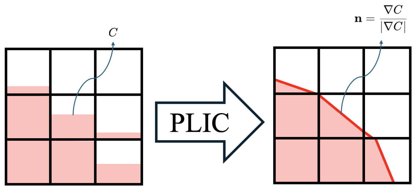
Figure 1. Illustration of PLIC reconstruction.
Fluids 11 00152 g001
Figure 2. Illustration for the calculation of flux integral advected from left. (Red: liquid phase; White: gas phase).
Fluids 11 00152 g002
Figure 3. Size distribution of raindrops from [47].
Fluids 11 00152 g003
Figure 4. Generation of 20 raindrops using stratified sampling approach.
Fluids 11 00152 g004
Figure 5. Initial state ( t = 0 ) for a shock tube with the interface between the high-pressure liquid water and low-pressure air at x 0 .
Fluids 11 00152 g005
Figure 6. Comparison between analytical and numerical solutions for N c e l l = 1000 , 2000 , 4000 , 8000 for density of the 1D two-phase shock tube at t = 229 μs (van Leer, CFL = 0.1 ).
Fluids 11 00152 g006
Figure 7. Comparison between analytical and numerical solutions for N c e l l = 1000 , 2000 , 4000 , 8000 for velocity of the 1D two-phase shock tube at t = 229 μs (van Leer, CFL = 0.1 ).
Fluids 11 00152 g007
Figure 8. Comparison between analytical and numerical solutions for N c e l l = 1000 , 2000 , 4000 , 8000 for pressure of the 1D two-phase shock tube at t = 229 μs (van Leer, CFL = 0.1 ).
Fluids 11 00152 g008
Figure 9. Initial conditions for shock wave in air/helium bubble interaction.
Fluids 11 00152 g009
Figure 10. Mach number contours and numerical Schlieren ( 1 + C 2 ) log 10 ( | ρ | + 1 ) of shock wave in air/helium bubble interaction at t = 100 μs, 800 × 800 cells.
Fluids 11 00152 g010
Figure 11. Mach number contours and numerical Schlieren ( 1 + C 2 ) log 10 ( | ρ | + 1 ) of shock wave in air/helium bubble interaction at t = 120 μs, 800 × 800 cells.
Fluids 11 00152 g011
Figure 12. Mach number contours and numerical Schlieren ( 1 + C 2 ) log 10 ( | ρ | + 1 ) of shock wave in air/helium bubble interaction at t = 160 μs, 800 × 800 cells.
Fluids 11 00152 g012
Figure 13. Mach number contours and numerical Schlieren ( 1 + C 2 ) log 10 ( | ρ | + 1 ) of shock wave in air/helium bubble interaction at t = 200 μs, 800 × 800 cells.
Fluids 11 00152 g013
Figure 14. (a) Numerical Schlieren ( 1 + C 2 ) log 10 ( | ρ | + 1 ) of shock wave in air/helium bubble interaction at t t 0 = 52 μs, where the dashed line is the initial shape of the helium bubble; (b) experimental result from [49] at 52 μs.

Fluids 11 00152 g014
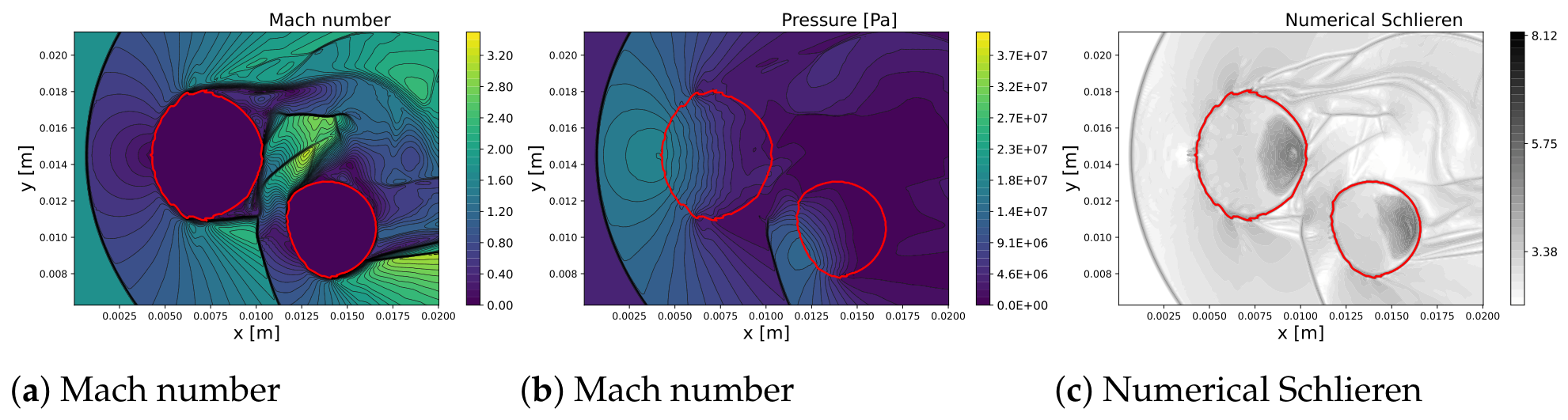
Figure 15. (a) Numerical Schlieren ( 1 + C 2 ) log 10 ( | ρ | + 1 ) of shock wave in air/helium bubble interaction at t t 0 = 72 μs, where the dashed line is the initial shape of the helium bubble; (b) experimental result from [49] at 72 μs.
Fluids 11 00152 g015
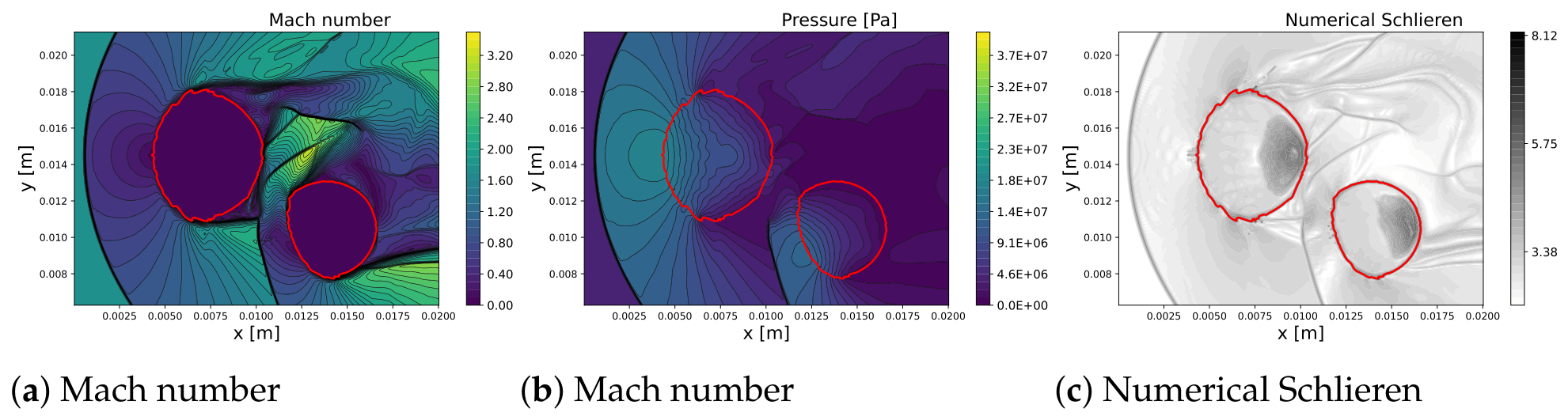
Figure 16. (a) Numerical Schlieren ( 1 + C 2 ) log 10 ( | ρ | + 1 ) of shock wave in air/helium bubble interaction at t t 0 = 102 μs, where the dashed line is the initial shape of the helium bubble; (b) experimental result from [49] at 102 μs.
Fluids 11 00152 g016
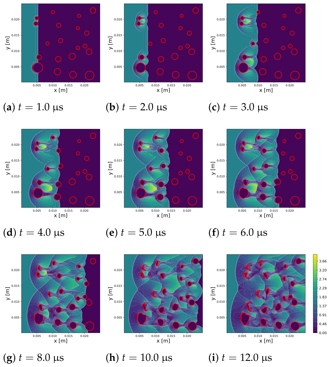
Figure 17. Initial conditions for shock wave interacting with one raindrop.
Fluids 11 00152 g017
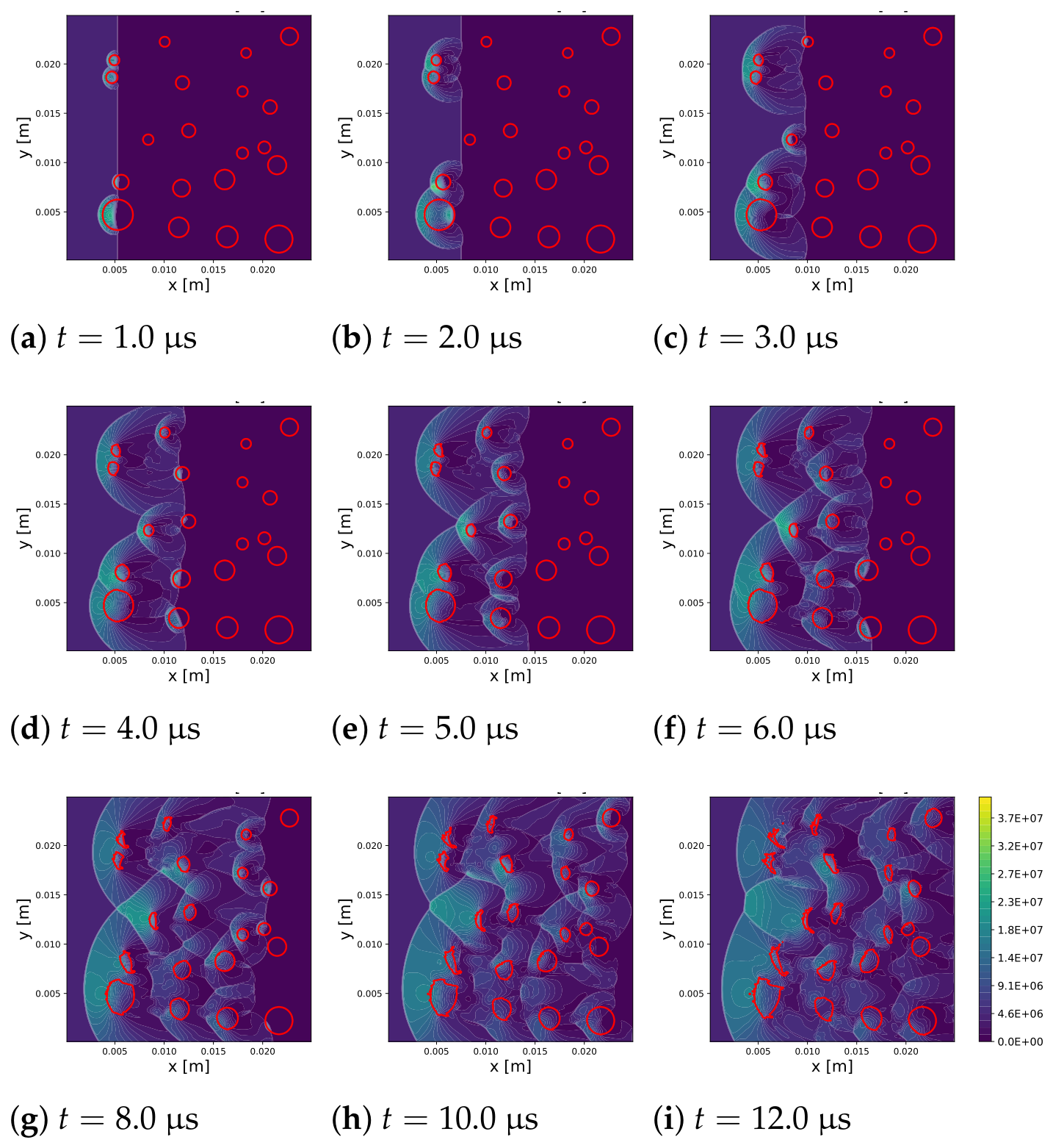
Figure 18. Pressure contours and numerical Schlieren 1 + α w a t e r 2 log 10 ( | ρ | + 1 ) of shock wave interacting with one raindrop at t = 1.0 μs.
Fluids 11 00152 g018
Figure 19. Pressure contours and numerical Schlieren 1 + α w a t e r 2 log 10 ( | ρ | + 1 ) of shock wave interacting with one raindrop at t = 10.0 μs.
Fluids 11 00152 g019
Figure 20. Pressure contours of shock wave in air and droplet interaction at t = 1 μs, t = 2 μs, and t = 3 μs with a 1000 × 1000 cell grid.
Fluids 11 00152 g020
Figure 21. Pressure contours of shock wave in air and droplet interaction at t = 1 μs, t = 2 μs, and t = 3 μs from [50].
Fluids 11 00152 g021
Figure 22. Pressure contours of shock wave in air and droplet interaction at t = 4 μs, t = 6 μs, and t = 8 μs with a 1000 × 1000 cell grid.
Fluids 11 00152 g022
Figure 23. Pressure contours of shock wave in air and droplet interaction at t = 4 μs, t = 6 μs, and t = 8 μs from [50].
Fluids 11 00152 g023
Figure 24. Pressure contours of shock wave in air and droplet interaction from t = 0 μs to t = 8 μs with a 1000 × 1000 cell grid.
Fluids 11 00152 g024
Figure 25. Numerical Schlieren ( 1 + C 2 ) log 10 ( | ρ | + 1 ) images of shock wave in air and droplet interaction from t = 0 μs to t = 8 μs with a 1000 × 1000 cell grid.
Fluids 11 00152 g025
Figure 26. Total mass error of the droplet over time during the shock wave in air and droplet interaction.
Fluids 11 00152 g026
Figure 27. Initial conditions for shock wave interacting with two raindrops.
Fluids 11 00152 g027
Figure 28. Mach number, pressure contours and numerical Schlieren log 10 ( | ρ | + 1 ) of shock wave interacting with two raindrops at t = 1.5 μs.
Fluids 11 00152 g028
Figure 29. Mach number, pressure contours and numerical Schlieren log 10 ( | ρ | + 1 ) of shock wave interacting with two raindrops at t = 4.0 μs.
Fluids 11 00152 g029
Figure 30. Mach number, pressure contours and numerical Schlieren log 10 ( | ρ | + 1 ) of shock wave interacting with two raindrops at t = 5.0 μs.
Fluids 11 00152 g030
Figure 31. Mach number, pressure contours and numerical Schlieren log 10 ( | ρ | + 1 ) of shock wave interacting with two raindrops at t = 7.0 μs.
Fluids 11 00152 g031
Figure 32. Mach number, pressure contours and numerical Schlieren log 10 ( | ρ | + 1 ) of shock wave interacting with two raindrops at t = 8.0 μs.
Fluids 11 00152 g032
Figure 33. Mach number, pressure contours and numerical Schlieren log 10 ( | ρ | + 1 ) of shock wave interacting with two raindrops at t = 9.0 μs.
Fluids 11 00152 g033
Figure 34. Mach number, pressure contours and numerical Schlieren log 10 ( | ρ | + 1 ) of shock wave interacting with two raindrops at t = 10.0 μs.
Fluids 11 00152 g034
Figure 35. Mach number, pressure contours and numerical Schlieren log 10 ( | ρ | + 1 ) of shock wave interacting with two raindrops at t = 11.5 μs.
Fluids 11 00152 g035
Figure 36. Mach number, pressure contours and numerical Schlieren log 10 ( | ρ | + 1 ) of shock wave interacting with two raindrops at t = 12.5 μs.
Fluids 11 00152 g036
Figure 37. Mach number evolution of shock wave interacting with twenty raindrops.
Fluids 11 00152 g037
Figure 38. Pressure [Pa] evolution of shock wave interacting with twenty raindrops.
Fluids 11 00152 g038
Table 1. Relative error of liquid mass for the 1D two-phase shock tube for different schemes and N c e l l with C F L = 0.1 .
N cell First OrderMinmodvan Leer
1000 0.00457 % 0.00492 % 0.00456 %
2000 0.00444 % 0.00433 % 0.00412 %
4000 0.00457 % 0.00439 % 0.00428 %
8000 0.00553 % 0.00457 % 0.00452 %
Disclaimer/Publisher’s Note: The statements, opinions and data contained in all publications are solely those of the individual author(s) and contributor(s) and not of MDPI and/or the editor(s). MDPI and/or the editor(s) disclaim responsibility for any injury to people or property resulting from any ideas, methods, instructions or products referred to in the content.