Abstract
Traditional hybrid RANS/LES methods often struggle to accurately capture both the boundary layer transition and flow separation simultaneously due to their reliance on fully turbulent RANS models. To address this limitation, the present study first evaluates three transitional RANS models (γ-Reθt-SST, γ-SST, and Kγ-SST) on the E387 airfoil. The results demonstrate that the γ-SST model offers the best balance of accuracy and computational efficiency in predicting laminar separation bubbles (LSBs) and transition points. Building on this, we implement the γ-SST-IDDES model into OpenFOAM-v2312, which integrates the γ-SST transitional RANS model with the Improved Delayed Detached Eddy Simulation (IDDES) approach. This coupling allows for the simultaneous prediction of the laminar-turbulent transition and high-fidelity resolution of separated flows. The γ-SST-IDDES model is rigorously validated across three airfoil cases with distinct separation characteristics: E387 (small separation), DBLN-526 (moderate separation), and NACA 0021 (massive separation). The results show that the γ-SST-IDDES model outperforms conventional methods, capturing leading-edge LSBs with high accuracy compared to fully turbulent IDDES. Additionally, it successfully resolves complex 3D vortical structures in separated regions, whereas unsteady URANS provides only quasi-2D results.
1. Introduction
Accurate prediction of boundary layer transition and separated flows is a critical challenge in computational fluid dynamics (CFD), particularly for aerodynamic applications such as wind turbine blades and aircraft wings. For example, modern wind turbine blades often employ blunt trailing-edge airfoils to enhance structural stability and aerodynamic performance. These airfoils are prone to complex flow phenomena, including boundary layer transition and massive flow separation, which significantly impact aerodynamic efficiency and load distributions. Traditional CFD methods, such as fully turbulent Reynolds-Averaged Navier–Stokes (RANS) models, fail to capture these phenomena due to their inherent assumption of a fully turbulent flow. While high-fidelity methods like Direct Numerical Simulation (DNS) and Large Eddy Simulation (LES) can resolve these flows, their prohibitive computational cost makes them impractical for industrial applications, especially at high Reynolds numbers.
To address the limitations of fully turbulent RANS models in predicting the boundary layer transition, researchers have developed transitional RANS models that incorporate transition mechanisms into traditional turbulence frameworks. Among these, Local Correlation-based Transition Models (LCTMs) have gained widespread acceptance due to their ability to predict natural, bypass, and separation-induced transitions using local variables. A pioneering example is the γ-Reθt-SST model proposed by Menter et al. [1,2,3,4], which introduced transport equations for intermittency (γ) and the momentum-thickness Reynolds number (Reθt) to model transition onset and progression. This model has been successfully applied to a wide range of aerodynamic configurations, including airfoils and turbomachinery blades [2,4]. Building on this foundation, subsequent advancements, such as the γ-SST model [5] and the Kγ-SST model [6], further simplified the formulation by reducing the number of transport equations or replacing them with algebraic expressions. These models have demonstrated improved accuracy in predicting transition points and flow separation in attached flows. However, their performance in massively separated flows remains limited, as the inherent averaging process of RANS formulations tends to produce predominantly two-dimensional flow structures, failing to capture the complex three-dimensional vortices characteristic of separated regions.
In parallel, hybrid RANS/LES methods have emerged as a promising approach to resolve separated flows with greater fidelity. Methods such as Detached Eddy Simulation (DES) and Improved Delayed Detached Eddy Simulation (IDDES) [7,8,9] combine the efficiency of RANS for boundary layer resolution with the accuracy of LES in separated regions. These methods have shown significant potential in capturing complex turbulent structures, particularly in massively separated flows. However, most existing hybrid methods are coupled with fully turbulent RANS models, which neglect the transition process and thus fail to accurately predict the boundary layer transition and its interaction with separation.
Recent efforts have sought to develop new turbulence modeling techniques that incorporate the benefits of both transitional RANS and LES approaches to simulate engineering or industrial flows more effectively. These new models aim to overcome the limitations of traditional hybrid RANS/LES methods in capturing the boundary layer transition while also reducing the high computational cost associated with LES, thereby providing a more accurate and efficient approach for predicting complex turbulent flows in practical applications. These efforts are listed in Table 1. Sorensen et al. [10] coupled the γ-Reθt-SST RANS model and the DES (detached-eddy simulation) model to predict the drag crisis of a circular cylinder. They discovered that this kind of DES-γ-Reθt model performed better than the fully turbulent DES model. Cui [11] coupled the IDDES model and the γ transition model to study the transition and separation past a wind-turbine airfoil near stall. Kwon and You [12] proposed a blending function to smoothly combine the γ-Reθt-SST RANS model with the SAS (scale adaptive simulation) or DES model to simulate the supercritical flow past a circular cylinder. Qiao et al. [13] applied the γ-Reθt-DDES (delayed detached-eddy simulation) model to simulate the attached flow past a flat plane. Yi et al. [14] adopted a γ-Reθt-IDDES (Improved Delayed Detached Eddy Simulation) model to predict the roughness-induced transition at hypersonic speed. Xiao et al. [15] coupled the k-ω-γ RANS model with the DDES model to simulate the transition and massively separated flow past the Orion capsule at hypersonic speed. Fu and Wang et al. [16] applied the DES-k-ω-γ model to predict the flow in turbomachinery. Sa [17] combined the DDES model and the γ-Reθt transition model to simulate the low-Reynolds-number flow around an Eppler 387 wing. Lin Zhou et al. [18] also applied the DDES-γ-Reθt coupling model to the separated transitional flow over the A-airfoil, DBLN-526 airfoil, and a circular cylinder in subcritical and critical regimes.

Table 1.
List of hybrid RANS/LES methods coupled with transitional RANS models.
OpenFOAM-v2312 is an open-source CFD software package. Currently, it includes only the γ-Reθt-SST transitional model. In this study, we first implement the γ-SST and Kγ-SST transitional RANS models and then evaluate all three transitional RANS models on the E387 airfoil to identify the most accurate and computationally efficient model for predicting the boundary layer transition. Next, we develop a transitional IDDES method, referred to as γ-SST-IDDES, by coupling the γ-SST transitional RANS model with IDDES. This hybrid framework is designed to simultaneously capture the boundary layer transition and resolve massively separated flows, addressing a critical limitation of existing methods. The proposed model is rigorously validated across three airfoil cases with distinct separation characteristics: the E387 airfoil (small separation), the DBLN-526 airfoil (moderate separation), and the NACA0021 airfoil (massive separation). These test cases are selected to assess the model’s capability to handle a wide range of flow conditions, from mild separations near the leading edge to massive separations at high angles of attack.
2. Numerical Methodology
2.1. Baseline Governing Equations
The k-ω Shear Stress Transport (SST) turbulence equations are used as the baseline governing equations [19,20]. The SST turbulence model has been employed to calculate the turbulent viscosity (μt) within the momentum and energy equations, to model the turbulence effects on the flow. The equations for the turbulent kinetic energy (k) and the specific dissipation rate are defined by Equations (1) and (2).
where ρ is the density, μ is the dynamic viscosity, and uj is the flow velocity. The production and destruction terms for the k equation are defined by Equations (3) and (4), respectively.
2.2. Transitional RANS Models
2.2.1. kOmegaSSTLM (γ-Reθt-SST)
The kOmegaSSTLM (γ-Reθt-SST) model proposed by Menter et al. [1,2,3,4] contains two new transport equations—the momentum-thickness Reynolds number and intermittency (γ), represented by Equations (5) and (6), respectively.
where are the destruction and transition source defined by Equations (7) and (8), respectively.
where Flength and FOnset are dimensionless functions that are used to control the intermittency equation within the boundary layer, and both of these functions are dependent on .
Finally, γ- equations interact with the kinetic energy equation (Equation (1)) of the SST model, resulting in a modified kinetic energy equation for the γ-Reθt-SST model, which takes the form of Equation (9).
where Pk,RANS and Dk,RANS are the original production and destruction terms for the kωSST model in Equations (3) and (4), respectively.
2.2.2. γ-SST
The γ-SST transition model was proposed by Menter et al. [5]. This transitional model consists of only one transport equation for the intermittency (γ), Equation (10).
where the transition source term is defined as
The magnitude of this source term is controlled by the transition length function, Flength, which used to be a correlation [4], but has been changed to a constant value of 100 [5]. The formulation of the function Fonset is used to trigger intermittency production. It contains the ratio of the local vorticity Reynolds number (Rev) to the critical Reynolds number ). The transition onset is controlled by the following functions:
The γ-SST model is finally obtained by coupling the γ equation with the SST turbulence. The new turbulence kinetic energy k equation of γ-SST is defined by Equation (13).
where Pk,RANS and Dk,RANS are the original production and destruction terms for the kωSST model in Equations (3) and (4), respectively.
2.2.3. Kγ-SST
The transition model was proposed by Sandhu et al. [6]. The Kγ-ωSST transitional model is derived from γ-kωSST; however, it uses a simple algebraic term, as shown in Equation (15), to estimate the intermittency using the turbulent Reynolds number (RT) instead of transport equations.
Furthermore, the transition model interacts with the turbulent kinetic energy equation (Equation (1)), leading to the modification of the kinetic energy equation into the following form:
where represent the production, destruction, and diffusion terms in the transport equation of the variable , respectively. The source terms are defined as follows:
More comprehensive information regarding this transitional model can be found in reference [6].
2.3. Improved Delayed Detached Eddy Simulation (IDDES) Formulations
IDDES is a type of DES-hybrid RANS/LES method [21,22], which possesses the capability to adaptively employ either DDES [23] or WMLES (Wall-Modeled LES) functionalities in different flow regions. In areas dominated by vortices, DDES length scales are implemented to eliminate grid scale dependence in the original DES methods, and in the near-wall regions, the WMLES model is employed to accurately capture boundary-layer profiles and eliminate the log-layer mismatch problem commonly encountered in DES hybrid methods. Consequently, the IDDES model combines the strengths of both DDES and WMLES techniques, resulting in improved predictions of small separation flows compared to the previous methods.
In the construction of RANS/LES hybrid methods, the grid scale in the LES methods is introduced into turbulence models. The LES-type grid scale is given by
where Cw is taken as 0.15; dw is the wall distance; hmax is the maximum cell length in three directions, which is the same definition as the original DES; and hwn is the normal cell height near the surface walls. The DDES length scale is formulated as hybrid RANS and LES length scales, incorporating a flow-dependent blending function (fd) which effectively prevents the LES mode from switching early in locally refined boundary-layer meshes [24].
where the blending function () is smooth in the transition area from the RANS to LES mode and given by
where
The WMLES length scale is defined as
where is another blending function defined as
The IDDES length scale is a combination of DDES and WMLES length scales, which is given as
2.3.1. kωSST-IDDES Formulation
The kωSST-IDDES model combines the fully turbulent RANS model kωSST with the IDDES model. In kωSST-IDDES, the length scale of RANS (lRANS) in the destruction term of the turbulent kinetic energy equation (Equation (1)) is eventually replaced with the length scale of IDDES (lIDDES) given in Equation (24).
Hence, the k equation of kωSST-IDDES is represented by Equation (26):
where Pk,RANS is the original production term for the kωSST model in Equation (3).
2.3.2. γ-kωSST-IDDES Formulation
The γ-kωSST-IDDES model couples the transitional RANS γ-kωSST with the IDDES model. It is ultimately derived by substituting the lRANS of the destruction term in the kinetic energy equation (Equation (13)) of the γ-kωSST model with the lIDDES represented by Equation (22). Equation (27) represents the new kinetic energy equation of the γ-kωSST-IDDES model, while the ω equation remains unchanged.
3. Numerical Results and Discussion
3.1. Two-Dimensional Simulations Around E387 Airfoil
The simulations are performed on the two-dimensional E387 airfoil test-case in accordance with the published wind tunnel test by McGhee et al. [25]. The details of the experimental flow parameters are presented in Table 2, which are strictly satisfied in the numerical simulations.
Table 2.
Flow parameters and working conditions.
Figure 1 depicts the “CO-grid” mesh topology that is used in the computational area. The first layer spacing is set to 2.0 × 10⁻⁵ to make sure y+ < 1. A small O-grid is generated with growing boundary layers around the E387 airfoil, as illustrated in Figure 1a. The diameter of the O-grid is three times that of the chord (c) of the airfoil. The expansion ratio from the first layer to the O-grid boundary is set to 1.2 and is constant for both the leading and trailing edges. The C-grid expansion begins from the last cell size of the O-grid, continuing with the same ratio. The C-grid is extended to 20c in the upstream direction and 40c in the downstream direction and is located outside of the O-grid. Since all the simulations are two-dimensional, the CO-grid is extruded with one chord (c) length by one spanwise layer in the spanwise direction.

Figure 1.
CO-grid on E387 two-dimensional test case: (a) CO-grid around airfoil; (b) Zoomed in O-grid around.
A pressure-based, incompressible steady flow solver, simpleFOAM, is used to perform the two-dimensional simulations. It employs the well-established SIMPLE algorithm [26] within the finite volume framework to solve the steady-state incompressible Navier–Stokes equations, with pressure–velocity coupling handled by the SIMPLE procedure. A steady-state approach is used for the time derivative term. Spatial discretization employs the 2nd cell-limited Gauss linear scheme for all gradient calculations in order to maintain numerical stability. For the divergence terms, a bounded Gauss linear upwind scheme based on velocity gradients is applied to the momentum equations, while viscous stress terms use the Gauss linear scheme. Different boundary conditions are assigned for different patches and linear solvers as represented by Table 3 and Table 4, respectively.
Table 3.
Boundary conditions.
Table 4.
Linear Solvers.
Four meshes, designated as mesh AA, mesh BB, mesh CC, and mesh DD, have been created for the purpose of conducting a grid convergence study, as outlined in Table 5. There are 110, 288, 344, and 544 wrap-around points on the surface of the airfoil, respectively. Figure 2 shows that the pressure coefficient (Cp) distributions on the airfoil’s surface are presented at an angle of attack of 0° with the γ-kωSST transitional model. It is observed that the Cp curve exhibits good convergence with the experimental data, and mesh CC and mesh DD demonstrate a high degree of similarity. Consequently, mesh CC has been selected for the simulations of other angle of attacks.
Table 5.
Details of the grid.
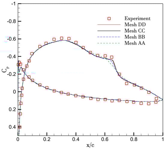
Figure 2.
Grid convergence study for E387 airfoil at 0°.
Figure 3 presents the pressure coefficient (Cp) curve of the E387 airfoil at α = 2°. Figure 4 depicts the streamlines near the laminar separation bubble (LSB). The positions of the Laminar Separation Point (LS) and Turbulent Reattachment Point (TR) are determined and the corresponding results are presented in Table 6. It is observed that the kωSSTLM model offers the most accurate estimation of the transition point within the LSB followed by γ-kωSST and Kγ-ωSST, respectively.
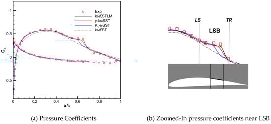
Figure 3.
Coefficient of pressure of an E387 airfoil at α = 2°: (a) Pressure Coefficients; (b) Zoomed-In pressure coefficients near LSB.
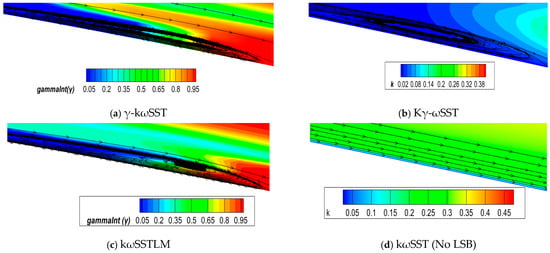
Figure 4.
LSB on upper surface of E387 airfoil at α = 2°: (a) γ-kωSST; (b) Kγ-ωSST; (c) kωSSTLM; (d) kωSST (No LSB).
Table 6.
Details of the LSB at α = 2°.
Figure 5 illustrates the Cp curve for the E387 airfoil at α = 4°. Table 7 summarizes the computational result of the LSB span and transition location estimated by each transitional model, as represented by Figure 6. When comparing the LS point at α = 4° with that at α = 2°, an apparent forward shift in the LSB, towards the leading edge, is observed. The kωSSTLM model estimates an LSB shift of 0.064 x/c, the γ-kωSST model predicts a shift of 0.077 x/c, and the Kγ-ωSST model anticipates a shift of 0.062 x/c.
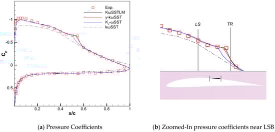
Figure 5.
Coefficient of pressure of an E387 airfoil at α = 4°: (a) Pressure Coefficients; (b) Zoomed-In pressure coefficients near LSB.
Table 7.
Details of the LSB at α = 4°.
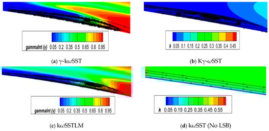
Figure 6.
LSB on upper surface of E387 airfoil at α = 4°: (a) γ-kωSST; (b) Kγ-ωSST; (c) kωSSTLM; (d) kωSST (No LSB).
Figure 7 illustrates the Cp curve for the E387 airfoil at α = 6°. At this particular α, the Kγ-ωSST model fails to capture the LSB streamlines, as they entirely vanish. However, the γ-kωSST and kωSSTLM models successfully captured the LSB streamlines, as represented in Figure 8. Table 8 summarizes the computational results of the LSB span and transition location. Upon comparing the transition behavior between α = 2° and α = 6°, it is observed that the LSB moves even closer towards the leading edge. The kωSSTLM model estimates a forward LSB shift of 0.12 x/c, while the γ-kωSST model predicts a shift of 0.133 x/c.
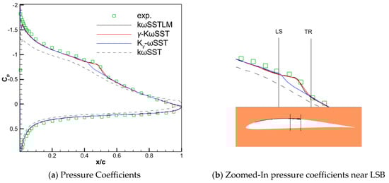
Figure 7.
Coefficient of pressure of an E387 airfoil at α = 6°: (a) Pressure Coefficients; (b) Zoomed-In pressure coefficients near LSB.
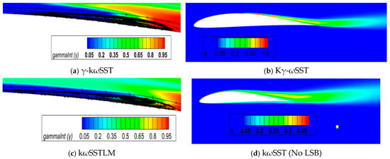
Figure 8.
LSB on upper surface of E387 airfoil at α = 6°: (a) γ-kωSST; (b) Kγ-ωSST; (c) kωSSTLM; (d) kωSST (No LSB).
Table 8.
Details of the LSB at α = 6°.
The results from this 2D test case show that the LSB shifts forward towards the leading edge when the angle of attack is increased. Furthermore, the kωSSTLM and γ-kωSST transitional models produced comparable results with a slight deviation. Therefore, in this paper, the γ-kωSST transitional model is employed to couple with IDDES.
3.2. IDDES and URANS Simulations
All the IDDES and URANS simulations are carried out using the rhoPimpleFoam solver within the OpenFOAM v2312. This solver implements the PIMPLE algorithm, which is a combination of the SIMPLE [27] and PISO [28] algorithms. This approach computes a transient and compressible solution, offering greater stability than the PISO algorithm alone and allowing for the use of larger time steps. The rhoPimpleFoam solver employs the finite volume method for numerical representation of the compressible three-dimensional Navier–Stokes equations. As suggested by Robertson [29], a standard three-level second-order backward difference is used for the time marching scheme. For spatial discretization, the 2nd-order cell-based scalar-limiting central difference is used for the gradient term; the 2nd-order bounded central difference is used for the divergence scheme; and the 2nd-order limited deferred correction scheme is used for the Laplacian scheme. In order to speed up the calculations, the message passing interface (MPI) is used for parallel computing.
The numerical test cases involve transitional flow over the E387 airfoil, DBLN-526 airfoil, and NACA0021 airfoil. These cases include a range of separation behaviors, small separation for the E387 airfoil, moderate separation for the DBLN-526 airfoil, and massive separation for the NACA0021 airfoil, to evaluate the performance of -kωSST-IDDES in separated transitional flows.
3.2.1. Flow over an E387 Airfoil
Jeong Hwan Sa et al. [17] used the E387 airfoil to verify their -DDES model. Their observations revealed that both the transitional IDDES model and the fully turbulent IDDES model generated the LSB at the leading edge because of the small separation. The transitional IDDES model produced an LSB size ranging from x/c = 0.025 to x/c = 0.091, while the fully turbulent IDDES model produced an LSB ranging from x/c = 0.004 to x/c = 0.043.
The numerical simulations are performed to simulate the flow over the E387 airfoil at an angle of attack of and a Reynolds number of 1 105. The freestream turbulence intensity is specified as The “CO-grid” mesh topology is adopted in the computational domain as shown in Figure 9. A small O-grid is generated with 524 points in the circumferential direction, 311 points on the suction side and 213 points on the pressure side, along with 101 points in the normal direction, with the diameter of this O-grid being 3c. The first cell normal to the wall is placed at 1 10−5c, so that y+ < 0.8. The C-grid is positioned on the outside of the O-grid and extends to 25c in the upstream direction and 40c in the downstream direction, with 51 and 101 grid points in the respective directions. The spanwise width is set to z/c = 0.2, and three sets of grids with Nz = 25, Nz = 35, and Nz = 49 are generated to study the effect of spanwise grid resolution. A non-dimensional time step size = 0.001 is used for all unsteady time-accurate computations. A total of 15 non-dimensional time units are computed, and the time-averaged solutions were obtained by taking the average over the last seven non-dimensional time units. The boundary conditions and the linear solver settings in OpenFOAM-v2312 for IDDES and URANS simulations in this paper are detailed in Table 9 and Table 10, respectively.
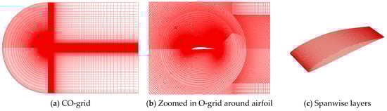
Figure 9.
CO-grid topology around E387 airfoil: (a) CO-grid; (b) Zoomed in O-grid around airfoil; (c) Spanwise layers.
Table 9.
Boundary conditions for IDDES and URANS simulations.
Table 10.
Linear Solver settings for IDDES and URANS simulations.
Figure 10 illustrates the distributions of the time-averaged surface pressure coefficient at three different numbers of grids. This Cp plot shows the best agreement with experimental data when Nz = 35. Therefore, Nz = 35 is selected for further simulations. Figure 11a,b depicts the time history of lift and drag coefficients, respectively, with the corresponding time-averaged force coefficients summarized in Table 11. It can be observed from this table that both simulations predict similar force coefficients, possibly due to the small angle of attack. However, the URANS: γ-kωSST simulation yields significantly lower values compared to the IDDES.
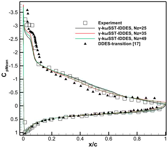
Figure 10.
Distribution of the pressure coefficient Cp of the time-averaged flow field for the E387 airfoil.
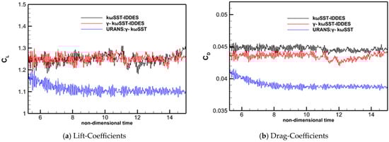
Figure 11.
Time history of lift and drag coefficient for E387 airfoil: (a) Lift-Coefficients; (b) Drag-Coefficients.
Table 11.
Comparisons of time-averaged CL and CD for E387 airfoil test case.
Figure 12 shows the vortex structure indicated by the Q = [(tr(∇U))2 − tr(∇U⋅∇U)] distributions. The URANS model exhibits small separation close to the leading edge, whereas the IDDES models generate intricate vortex formations. These vortex patterns, characteristic of Large Eddy Simulations, demonstrate the effective integration of the IDDES and transition model within the present -kωSST-IDDES model.
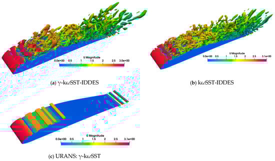
Figure 12.
Instantaneous flow field results for E387 airfoil test case (Q-criterion = 100 isosurface colored by the velocity magnitude): (a) γ-kωSST-IDDES; (b) kωSST-IDDES; (c) URANS: γ-kωSST.
Figure 13 shows the time-averaged streamlines near the LSB. The kωSST-IDDES yields a considerably smaller LSB when compared to the γ-kωSST-IDDES. Specifically, the LSB size produced by the γ-kωSST-IDDES ranges from x/c = 0.063 to x/c = 0.121, while the LSB generated by the kωSST-IDDES spans from x/c = 0.041 to x/c = 0.077.
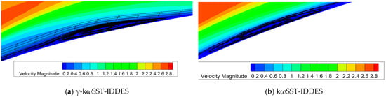
Figure 13.
Time-averaged streamlines near the laminar separation bubble for E387 airfoil: (a) γ-kωSST-IDDES; (b) kωSST-IDDES.
3.2.2. Flow over a DBLN-526 Airfoil
The DBLN-526 airfoil was first used by Lin Zhou et al. [18] to validate their -DDES transitional model along with a wind tunnel experiment at the NLF wind tunnel of Northwestern Polytechnical University. In the experiments, the transition point was observed near the leading edge at x/c 0.05, and the boundary layer separates around x/c 0.5.
In this section, numerical simulations are conducted to analyze the flow over the DBLN-526 airfoil at an angle of attack of with a chord-based Reynolds number of 0.8 106 and a turbulence intensity of 0.15%. The “CO-grid” mesh topology is also utilized for this test case in the computational domain as shown in Figure 14. A small O-grid is created with 568 points in the circumferential direction, comprising 287 points on the suction side and 281 points on the pressure side. Additionally, there are 141 points in the normal direction, and the diameter of this O-grid is set at 6 times the chord length (6c). The height of the first grid normal to the wall is placed at 1 10−5c, ensuring y+ < 1. The C-grid is situated outside the O-grid and extends to 25c in the upstream direction and 40c in the downstream direction, which consists of 81 grid points upstream and 141 grid points downstream. The spanwise width is extended to 0.5c, and four sets of grids with Nz = 31, Nz = 41, Nz = 45, and Nz = 51 are used. A non-dimensional time step size = 0.0018 is used for all unsteady time-accurate computations. The computations are carried out for a total of 10 non-dimensional time units. The time-averaged solutions are obtained by averaging the data over the last six non-dimensional time units.
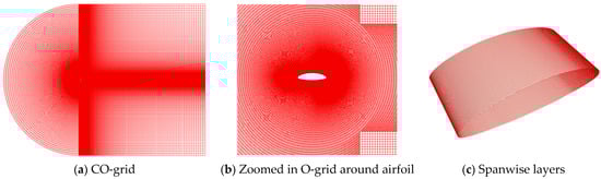
Figure 14.
CO-grid topology around DBLN-526 airfoil: (a) CO-grid; (b) Zoomed in O-grid around airfoil; (c) Spanwise layers.
Figure 15 shows the time-averaged surface pressure coefficient distribution at four different levels of grids. The present method,-kωSST-IDDES, shows the grid convergence beyond Nz = 41, and agrees well with the experiment and computation of Zhou [18]. Figure 16 shows the time histories of CL and CD. Table 12 shows the comparison of time-averaged CL and CD at different spanwise grid numbers, along with kωSST-IDDES and URANS: -kωSST. The significant improvement in the force coefficients can be clearly observed while using the transitional IDDES model over the fully turbulent IDDES model and the transitional URANS.
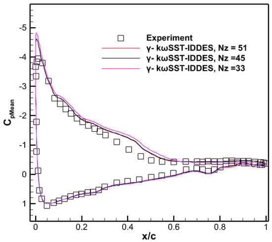
Figure 15.
Distribution of the pressure coefficient Cp of the time-averaged flow field for the DBLN-526 airfoil.
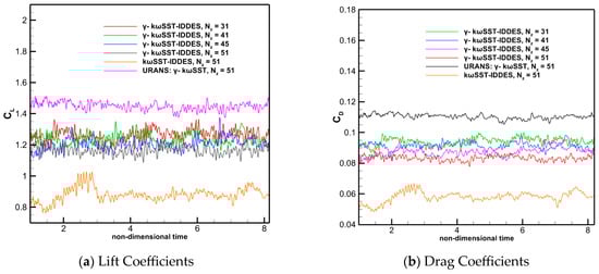
Figure 16.
Time histories of lift and drag coefficients for DBLN-526 airfoil: (a) Lift Coefficients; (b) Drag Coefficients.
Table 12.
Comparisons of time-averaged CL and CD for DBLN-526 airfoil test case.
Figure 17 compares the turbulent structures of IDDES and URANS. The URANS: -kωSST simulation illustrates the two-dimensional (2D) turbulent structures, whereas the IDDES produces highly complex three-dimensional (3D) structures that become slightly apparent with the increase in spanwise grid numbers. The shear layer instability induced by γ-kωSST-IDDES appears significantly further downstream compared to that induced by kωSST-IDDES, primarily due to the presence of a boundary layer transition. Both the γ-kωSST-IDDES and kωSST-IDDES predict the development of shear layer instabilities from quasi-2D large-scale structures to 3D small-scale turbulent structures.
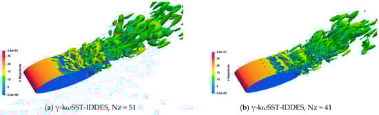
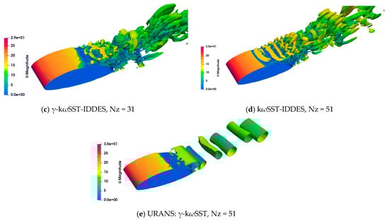
Figure 17.
Instantaneous flow field results for DBLN-526 airfoil test case (Q-criterion = 300 isosurface colored by the velocity magnitude): (a) γ-kωSST-IDDES, Nz = 51; (b) γ-kωSST-IDDES, Nz = 41; (c) γ-kωSST-IDDES, Nz = 31; (d) kωSST-IDDES, Nz = 51; (e) URANS: γ-kωSST, Nz = 51.
Figure 18 shows the time-averaged streamlines near the leading edge to capture the laminar separation bubble. The γ-kωSST-IDDES model produces the laminar separation bubble with laminar separation onset at x/c = 0.03 and turbulent reattachment at x/c = 0.0736 along with the transition point near the leading edge at x/c = 0.0567. kωSST-IDDES on the other hand does not give any LSB. Figure 19 shows the time-averaged streamlines near the boundary layer separation. The γ-kωSST-IDDES model captures the flow separation bubble with onset at x/c = 0.4400 and reattachment at x/c = 0.4736. However, kωSST-IDDES predicts no such separation bubble. Figure 20 compares the velocity profiles at different chordwise positions by the three simulation methods. The profiles from γ-kωSST-IDDES and URANS: γ-kωSST are quite similar, indicating that both models predict the transitional flow behavior and the LSB’s extent with reasonable accuracy, primarily due to their capability to capture the laminar-to-turbulent transition effectively. In contrast, the kωSST-IDDES method shows distinct deviations in the velocity profiles, suggesting a different representation of the boundary layer development, likely due to its inherent approach to modeling the turbulent flow without explicitly accounting for the transitional phenomena as the γ-based models do.
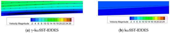
Figure 18.
Time-averaged streamlines near the boundary layer separation: (a) γ-kωSST-IDDES; (b) kωSST-IDDES.
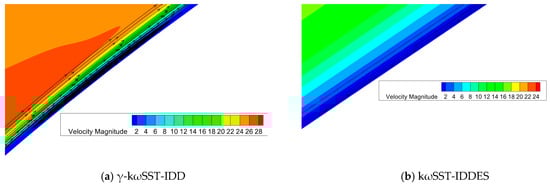
Figure 19.
Time-averaged streamlines near the laminar separation bubble: (a) γ-kωSST-IDDES; (b) kωSST-IDDES.
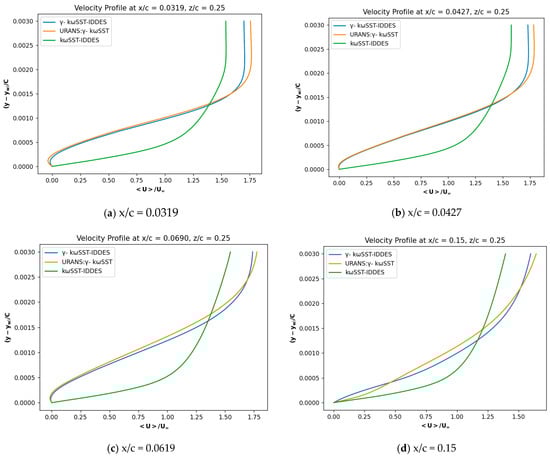
Figure 20.
The profiles of mean velocity at various x/c locations: (a) x/c = 0.0319; (b) x/c = 0.0427; (c) x/c = 0.0619; (d) x/c = 0.15.
3.2.3. Flow over an NACA0021 Airfoil
A common test case for massively separated flows is the flow over the NACA0021 airfoil at an angle of attack of . Wang et al. [29,30,31] employed this test case for fully turbulent IDDESs; however, it has not yet been utilized for transitional IDDESs.
In this study, numerical simulations are performed with a chord-based Reynolds number of 0.3 106, and a turbulence intensity of 0.03%. The same “CO-grid” mesh topology as previous test cases is used for this test case in the computational domain as shown in Figure 21. A small O-grid is created with 200 points in the circumferential direction and 101 points in the normal direction, and the diameter of this O-grid is set at six times the chord length (6c). The height of the first grid normal to the wall is placed at 1 10−5c, ensuring y+ < 1. The C-grid is situated outside the O-grid and extends to 25c in the upstream direction and 40c in the downstream direction, which consists of 41 grid points upstream and 67 grid points downstream. The spanwise width is extended to 1c, and three sets of grids with Nz = 28, Nz = 40, and Nz = 56 are used. A non-dimensional time step size = 0.00016 is used for all unsteady time-accurate computations. The computations were carried out for a total of five non-dimensional time units.
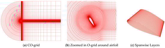
Figure 21.
“CO-grid” topology around NACA0021 airfoil test case: (a) CO-grid; (b) Zoomed in O-grid around airfoil; (c) Spanwise Layers.
Figure 22 shows the distribution of the pressure coefficient of the time-averaged flow field for the NACA0021 airfoil test case at three different levels of grids. It shows a good convergence with grid refinement and gives the best agreement with experimental data [32] at Nz = 40. Hence, the spanwise grid with Nz = 40 is used for the further numerical simulations. Figure 23 shows the comparison of time histories of CL and CD. Table 13 shows the comparison of time-averaged CL and CD between IDDES and URANS simulations at different spanwise grid numbers. The -kωSST-IDDES improves the lift and drag coefficients in comparison to both kωSST-IDDES and γ-kωSST. However, the force coefficient results obtained from URANS: γ-kωSST largely deviate from those of the IDDES results.
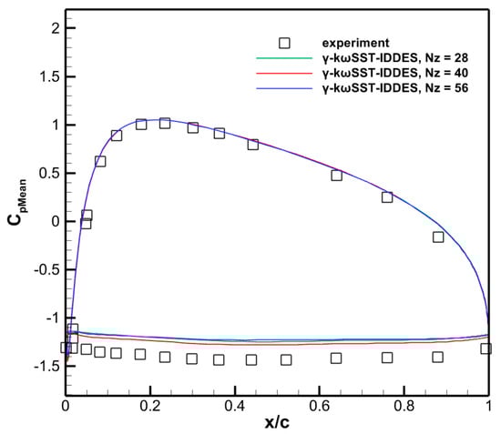
Figure 22.
Distribution of the pressure coefficient Cp of the time-averaged flow field for the NACA0021 airfoil test case.
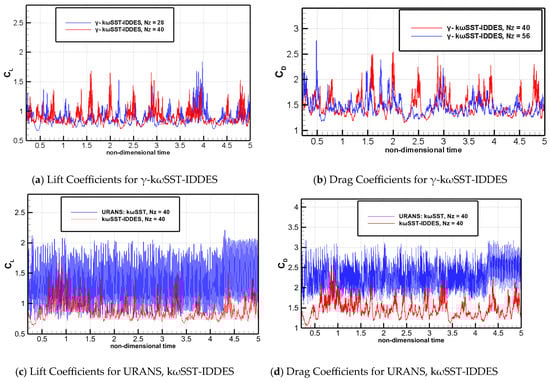
Figure 23.
Time histories of force coefficients for NACA0021 airfoil test case: (a) Lift Coefficients for γ-kωSST-IDDES; (b) Drag Coefficients for γ-kωSST-IDDES; (c) Lift Coefficients for URANS, kωSST-IDDES; (d) Drag Coefficients for URANS, kωSST-IDDES.
Table 13.
Comparisons of time-averaged CL and CD for NACA0021 airfoil test case.
Figure 24 shows the comparison of turbulent flow structures among the IDDES and URANS simulations. A distinction between the -kωSST-IDDES and the kωSST-IDDESs can be observed on the leading edge of the airfoil. There are fractures and the shear layer is completely detached in the leading edge of the airfoil in the kωSST-IDDES, whereas the shear layer is attached in the -kωSST-IDDES. Like the previous test cases, the URANS: -kωSST simulation produces two-dimensional vortex structures. Figure 25 illustrates the time-averaged streamlines near the laminar separation bubble. The γ-kωSST-IDDES model yields the LSB, manifesting onset at x/c = 0.0146 and reattachment at x/c = 0.0169, alongside the transition point at x/c = 0.0153. This demonstrates the ability of γ-kωSST-IDDES to effectively capture the transition properties within the flow field. Conversely, the kωSST-IDDES model fails to characterize any LSB, highlighting the limitation of this approach in capturing certain flow phenomena.
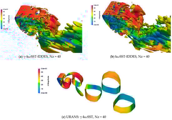
Figure 24.
Instantaneous flow field results for the NACA0021 airfoil test case (Q-criterion = 500 isosurface colored by the velocity magnitude): (a) γ-kωSST-IDDES, Nz = 40; (b) kωSST-IDDES, Nz = 40; (c) URANS: γ-kωSST, Nz = 40.
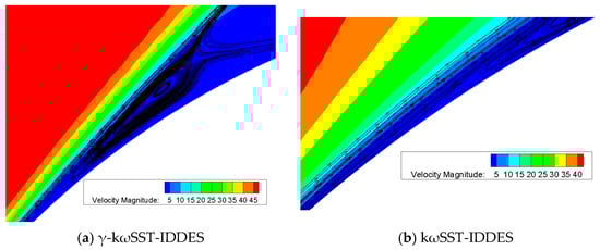
Figure 25.
Time-averaged streamlines near the laminar separation bubble: (a) γ-kωSST-IDDES; (b) kωSST-IDDES.
4. Conclusions
In this study, the γ-kωSST and Kγ-ωSST transitional models were newly implemented in OpenFOAM-v2312 to simulate the laminar–turbulent transition and laminar separation bubble (LSB) around the two-dimensional E387 airfoil at angles of attack of 2°, 4°, and 6°. As the angle of attack increases, the LSB is observed to move closer to the leading edge. The size of the LSB predicted by both the γ-kωSST and kωSSTLM models is nearly identical at each angle of attack. Based on these results, the γ-kωSST model was coupled with the traditional IDDES method to form a hybrid approach, referred to as γ-kωSST-IDDES, capable of capturing both transition and large-scale separation phenomena.
To evaluate the performance of the γ-kωSST-IDDES model, three airfoils with varying degrees of flow separation were studied: the E387 airfoil (small separation), the DBLN-526 airfoil (moderate separation), and the NACA0021 airfoil (massive separation). Across all test cases, both the γ-kωSST-IDDES and kωSST-IDDES models generated highly complex, three-dimensional turbulent structures, while the URANS-based γ-kωSST simulations produced predominantly two-dimensional structures.
For the E387 airfoil, both hybrid models captured an LSB near the leading edge, although the kωSST-IDDES predicted a significantly smaller bubble compared to γ-kωSST-IDDES. The γ-kωSST-IDDES predicted laminar separation at x/c = 0.063 and turbulent reattachment at x/c = 0.121. In the case of the DBLN-526 airfoil, the γ-kωSST-IDDES accurately predicted an LSB with laminar separation at x/c = 0.030 and reattachment at x/c = 0.0736, and additionally captured a secondary separation bubble at x/c = 0.4400, which was not resolved by the kωSST–IDDES model. Finally, for the NACA0021 airfoil, the γ-kωSST-IDDES predicted an LSB with onset at x/c = 0.0146 and reattachment at x/c = 0.0169, while the kωSST–IDDES again failed to capture this transition phenomenon.
Overall, the results demonstrate that the γ-kωSST-IDDES model provides improved predictive capability for transitional and separated flows, especially in cases with complex laminar-to-turbulent behavior and laminar separation bubbles.
Author Contributions
Conceptualization, S.G. and Y.W.; data curation, S.G.; formal analysis, S.G.; investigation, S.G.; methodology, S.G. and Y.W.; software, S.G.; validation, S.G.; visualization, S.G.; writing—original draft preparation, S.G.; resources, Y.W.; supervision, Y.W.; project administration, X.N.; funding acquisition, X.N.; Writing—review & editing, X.N. and Y.W. All authors have read and agreed to the published version of the manuscript.
Funding
This work was supported by the National Key Research and Development Program of China under Grant No. 2023YFB3002800 and the Natural Science Basic Research Plan in Shaanxi Province of China (Program No. 2023-JC-ZD-01).
Institutional Review Board Statement
Not applicable.
Informed Consent Statement
Not applicable.
Data Availability Statement
The data that support the findings of this study are available from the first author upon reasonable request.
Conflicts of Interest
The authors declare no conflicts of interest.
References
- Menter, F.R.; Esch, T.; Kubacki, S. Transition modeling based on local variables. In Proceedings of the 5th International Symposium on Engineering Turbulence Modelling and Measurements, Mallorca, Spain, 16–18 September 2002; pp. 555–564. [Google Scholar]
- Menter, F.R.; Langtry, R.B.; Likki, S.R.; Suzen, Y.B.; Huang, P.G.; Völker, S. A correlation-based transition model using local variables part 1–model formulation. J. Turbomach. 2006, 128, 413–422. [Google Scholar] [CrossRef]
- Menter, F.R.; Langtry, R.B.; Völker, S. Transition modeling for general purpose CFD codes. Flow Turbul. Combust. 2006, 77, 277–303. [Google Scholar] [CrossRef]
- Langtry, R.B.; Menter, F.R. Correlation-based transition modeling for unstructured parallelized computational fluid dynamics codes. AIAA J. 2009, 47, 2894–2906. [Google Scholar] [CrossRef]
- Menter, F.R.; Smirnov, P.E.; Liu, T.; Avancha, R. A one-equation local correlation-based transition model. Flow Turbul. Combust. 2015, 95, 583–619. [Google Scholar] [CrossRef]
- Sandhu, J.P.S.; Ghosh, S. A local correlation-based zero-equation transition model. Comput. Fluids 2021, 214, 104758. [Google Scholar] [CrossRef]
- Spalart, P.; Jou, W.; Strelets, M.; Allmaras, S. Comments on the feasibility of LES for wings, and on a hybrid RANS/LES approach, advances in DNS/LES. In Proceedings of the 1st AFOSR International Conference on DNS/LES, Ruston, LA, USA, 4–8 August 1997; Greden Press: Columbus, OH, USA, 1997. [Google Scholar]
- Charles, M. A Comprehensive Study of Detached-Eddy Simulation. Ph.D. Thesis, Technische Universität, Berlin, Germany, 2009. [Google Scholar]
- Spalart, P.R.; Deck, S.; Shur, M.L.; Squires, K.D.; Strelets, M.K.; Travin, A. A new version of detached-eddy simulation, resistent to ambiguous grid densities. Theor. Comput. Fluid Dyn. 2006, 20, 181–195. [Google Scholar] [CrossRef]
- Sørensen, N.N.; Bechmann, A.; Zahle, F. 3D CFD computations of transition flows using DES and a correlation-based transition model. Wind. Energy 2011, 14, 77–90. [Google Scholar] [CrossRef]
- Cui, W.; Xiao, Z.; Yuan, X. Simulations of transition and separation past a wind-turbine airfoil near stall. Energy 2020, 205, 118003. [Google Scholar] [CrossRef]
- You, J.Y.; Kwon, O.J. Blending of SAS and correlation-based transition models for flow simulation at supercritical Reynolds numbers. Comput. Fluids 2013, 80, 63–70. [Google Scholar] [CrossRef]
- Qiao, L.; Bai, J.Q.; Hua, J.; Wang, C. Combination of DES and DDES with a correlation-based transition model. Appl. Mech. Mater 2014, 444, 374–379. [Google Scholar] [CrossRef]
- Yi, M.; Zhao, H.; Le, J.; Xiao, B.; Zheng, Z. γ-Reθ transition model based on IDDES frame. Acta Aeronaut. Astronaut. Sin. 2019, 40, 122726. [Google Scholar]
- Xiao, Z.; Wang, G.; Yang, M.; Chen, L. Numerical investigations of hypersonic transition and massive separation past Orion capsule by DDES-Tr. Int. J. Heat Mass Tran. 2019, 137, 90–107. [Google Scholar] [CrossRef]
- Wang, L.; Mockett, C.; Fu, S.; Thiele, F. Turbomachinery flow simulations using a hybrid RANS/LES method combinedwith a RANS transition model. In Proceedings of the XXI International Symposium on Air Breathing Engines: ISABE Conference, Busan, Republic of Korea, 9–13 September 2013. [Google Scholar]
- Sa, J.H.; Park, S.H.; Kim, C.J.; Park, J.K. Low-Reynolds number flow computation for eppler 387 wing using hybrid DES/transition model. J. Mech. Sci. Technol. 2015, 29, 1837–1847. [Google Scholar] [CrossRef]
- Zhou, L.; Gao, Z.; Du, Y. Flow-dependent DDES/γ−Reθt coupling model for the simulation of separated transitional flow. Aerosp. Sci. Technol. 2019, 87, 389–403. [Google Scholar] [CrossRef]
- Park, S.H.; Kwon, J.H. Implementation of k-ω Turbulence Models in an Implicit Multi-grid Method. AIAA J. 2004, 42, 1348–1357. [Google Scholar] [CrossRef]
- Menter, F.R. Two-equation eddy-viscosity turbulence models for engineering applications. AIAA J. 1994, 32, 1598–1605. [Google Scholar] [CrossRef]
- Shur, M.L.; Spalart, P.R.; Strelets, M.K.; Travin, A.K. A hybrid RANS-LES approach with delayed-DES and wall-modelled LES capabilities. Int. J. Heat Fluid Flow 2008, 29, 1638–1649. [Google Scholar] [CrossRef]
- Gritskevich, M.S.; Garbaruk, A.V.; Schütze, J.; Menter, F.R. Development of DDES and IDDES Formulations for the k-Shear Stress Transport Model. Flow Turbul. Combust. 2012, 88, 431–449. [Google Scholar] [CrossRef]
- Fröhlich, J.; Von Terzi, D. Hybrid RANS/LES methods for the simulation of turbulent flows. Prog. Aerosp. Sci. 2008, 44, 349–377. [Google Scholar] [CrossRef]
- Huang, J.; Xiao, Z.; Liu, J.; Fu, S. Simulation of shock wave buffet and its suppression on an OAT15A supercritical airfoil by IDDES. Sci. China Phys. Mech. Astron. 2012, 55, 260–271. [Google Scholar] [CrossRef]
- Robert, J.M.; Betty, S.W.; Betty, F.M. Experimental Results for the Eppler 387 Airfoil at Low Reynolds Numbers in the Langley Low-Turbulence Pressure Tunnel. Tech. Rep. National Aeronautics and Space Administration. 1988. Available online: https://ntrs.nasa.gov/citations/19890001471 (accessed on 27 May 2025).
- Caretto, L.S.; Gosman, A.D.; Patankar, S.V.; Spalding, D.B. Two calculation procedures for steady, three-dimensional flows with recirculation. In Proceedings of the Third International Conference on Numerical Methods in Fluid Mechanics, Paris, France, 3–7 July 1972; Springer: Berlin/Heidelberg, Germany, 1973; pp. 60–68. [Google Scholar]
- Issa, R. Solution of the implicitly discretised fluid flow equations by operatorsplitting. J. Comput. Phys. 1986, 62, 40–65. [Google Scholar] [CrossRef]
- Robertson, E.; Choudhury, V.; Bhushan, S.; Walters, D.K. Validation of OpenFOAM numerical methods and turbulence models for incompressible bluff body flows. Comput. Fluids 2015, 123, 122–145. [Google Scholar] [CrossRef]
- Wang, Y.; Song, B.; Song, W.; Han, Z.H. Partially-averaged Navier-Stokes simulations of unsteady flow around NACA0021 airfoil at 60° angle of attack. In Proceedings of the 2018 Applied Aerodynamics Conference, Atlanta, GA, USA, 25–29 June 2018. [Google Scholar]
- Wang, Y.; Liu, K.; Song, W.P.; Han, Z.H. Scale adaptive simulations of unsteady flow around NACA0021 airfoil at 60° angle of attack. In Proceedings of the AIAA Scitech Forum, San Diego, CA, USA, 7–11 January 2019. [Google Scholar]
- Wang, Y.; Liu, K.; Han, Z. Detached eddy simulation on the flow around NACA0021 airfoil beyond stall using OpenFOAM. In Asia-Pacific International Symposium on Aerospace Technology; Springer: Singapore, 2018. [Google Scholar]
- El Akoury, R.; Braza, M.; Hoarau, Y.; Vos, J.; Harran, G.; Sevrain, A. Unsteady flow around a NACA0021 airfoil beyond stall at 60° angle of attack. In IUTAM Symposium on Unsteady Separated Flows and Their Control: Proceedings of the IUTAM Symposium “Unsteady Separated Flows and their Control“, Corfu, Greece, 18–22 June 2007; Springer: Dordrecht, The Netherlands, 2009; IUTAM Bookseries 14. [Google Scholar]
Disclaimer/Publisher’s Note: The statements, opinions and data contained in all publications are solely those of the individual author(s) and contributor(s) and not of MDPI and/or the editor(s). MDPI and/or the editor(s) disclaim responsibility for any injury to people or property resulting from any ideas, methods, instructions or products referred to in the content. |
© 2025 by the authors. Licensee MDPI, Basel, Switzerland. This article is an open access article distributed under the terms and conditions of the Creative Commons Attribution (CC BY) license (https://creativecommons.org/licenses/by/4.0/).