Particles in Homogeneous Isotropic Turbulence: Clustering and Relative Influence of the Forces Exerted on Particles

Abstract

A combination of lattice Boltzmann method (LBM)-based computations and Lagrangian particle tracking simulations is presented to study the dispersion and clustering of inertial particles in a forced homogeneous and isotropic turbulent flow and to analyze the relative importance of the various forces acting on particles. The particle dynamics are investigated across a wide range of particle-to-fluid density ratios (from 0.01 to 1000) and Stokes numbers (from 1.4 × 10⁻⁶ to 55.4), at a Taylor microscale Reynolds number of 33.6. Particle clustering is quantified using Voronoï tessellations. Results confirm that clustering intensity is maximized at Stokes numbers around unity, where particles preferentially accumulate in low-vorticity regions. Particle dynamics within the turbulent flow considered here vary fundamentally with density and size, even among tracer-like particles. Low-density and neutrally buoyant particles mimic tracers via either velocity matching or acceleration balance, while dense particles follow inertia-dominated dynamics.

1. Introduction

Turbulent flows with dispersed particles are encountered in numerous industrial applications and natural phenomena, including fuel or coal combustion, oil transport, liquid metal processing, sediment transport in rivers, and cloud dynamics [1,2,3,4,5]. In these systems, the continuous phase can either be a gas or a liquid: when it is a gas, transported particles are referred to as aerosols, and when it is a liquid, they are called hydrosols. Aerosols are characterized by a high particle-to-fluid density ratio, while in hydrosols, the particle-to-fluid density ratio is close to unity.

Because of the frequent occurrence and important role of multiphase flows, the modeling of the phenomena at play in these systems is a very active research field. One of the key concerns is, in particular, to better understand the dynamics of individual particles and their impact on the resulting distribution of the dispersed phase in space. An important phenomenon observed long ago in such systems and which continues to receive a lot of attention is the accumulation of inertial particles in specific regions, forming clusters, which results in an inhomogeneous particle concentration field [6]. This behavior, called preferential sampling or clustering, has important implications on various processes such as collision and coalescence kinetics. Clustering is known to strongly depend on the Stokes number ${\tau }_p^{+}$, defined as the ratio of the particle response time to the Kolmogorov time scale of the fluid flow, reaching a peak for Stokes numbers close to unity [7,8,9,10]. For relatively low Stokes numbers, clustering is traditionally attributed to the ejection of particles from vortex cores by centrifugation [7]. For large Stokes numbers, the precise mechanism causing clustering still lacks consensus, yet several studies have suggested that history effects may play a significant role [11].

The dynamics of individual small spherical particles in a non-uniform flow is governed by the Maxey and Riley equation [12], which was derived under the conditions of low particle Reynolds number. In this equation, the total hydrodynamic force acting on each particle consists of several contributions, including drag, added mass, pressure gradient, and the Basset history force. The significance of each of these contributions has been discussed in a number of numerical studies considering various flow conditions. Considering particles suspended in a turbulent channel flow with particle-to-fluid density ratios between 2.65 and 2650, Armenio and Fiorotto [13] reported that for large density ratios the added mass, pressure gradient, and Basset force are negligible compared to the drag, while for density ratios close to one, these forces become significant. Similarly, in a study dealing with the dispersion of dense particles in decaying isotropic turbulence, Elgobashi and Truesdell [14] found that drag is dominant. A detailed study of the relative significance of the forces acting on a population of particles in homogeneous isotropic turbulence (HIT) was conducted by Daitche [15] across a broad range of density ratios (from 0 to 1000). It showed that the contributions of added mass and pressure gradient are not negligible, their effects depending on both particle density and size. Olivieri et al. [16], considering density ratios between 1 and 1000, and Yokojima et al. [17], who studied particles with density ratios ranging from 0.01 to 100, both found that the pressure gradient and the added mass terms were significant for low density ratios up to 10. Conversely, for heavy particles (particle-to-fluid density ratio above 100), the drag force largely dominates, while the other forces become negligible.

The present paper numerically investigates the effect of various forces acting on the particles in a forced homogeneous isotropic turbulent flow. While most of the past studies refer to moderate to large particle-to-fluid density ratios. Here, we explore a wide range of density ratios, including very small values that have received little attention so far [13,17]. This contributes to filling a gap in the literature and provides a more comprehensive picture of the dynamics of such particles in turbulent flows. The choice of homogenous and isotropic turbulence is motivated by the need to focus on fundamental particle–turbulence interactions in a well-controlled and canonical flow configuration, which serves as a baseline before tackling more complex anisotropic or wall-bounded flows. This simplified setting also addresses the current lack of literature on hydrosols in turbulent flow. The structure of the paper is as follows. Section 2 introduces the mathematical models, the numerical methods, and the parameters of the numerical simulations. Section 3.1 focuses on the characterization of the turbulent flow field. Section 3.2 presents simulation results on the clustering phenomenon, which is analyzed by means of Voronoï tessellations. Section 3.3 quantifies the relative impact of the various forces acting on particles. Finally, Section 4 provides concluding remarks highlighting the new insights provided by this study.

2. Simulation Set-Up

The simulated domain is a 3D cubic box, with periodic boundary conditions applied in all directions. Direct numerical simulations (DNS) of homogeneous isotropic turbulence are conducted using the lattice Boltzmann method (LBM) by Eggels and Somers [18], which is described with more details in Sungkorn and Derksen [19]. Turbulence is induced by a local volume force, using two linear forcing models: one by Lundgren [20] and one by Carroll and Blanquart [21].

Particle trajectories are computed by Lagrangian tracking, considering perfectly smooth, solid, and spherical particles that are smaller than the smallest length scale of the flow.

2.1. Turbulent Flow

Two forcing models for generating homogeneous and isotropic turbulence have been employed: Lundgren’s linear forcing model [17] and the modified version proposed by Carroll and Blanquart [18]. Both models add a source term to the momentum equation in physical space to sustain turbulence by counteracting the natural decay of kinetic energy.

Lundgren’s original method injects energy into the flow field through a forcing term proportional to the fluctuating velocity. Since, in homogeneous and isotropic turbulence, there is no mean flow, the instantaneous velocity $\overrightarrow{u }$ only contains purely fluctuating contributions, justifying its direct use in the forcing term.

$${\displaystyle \frac{\partial \overrightarrow{u}}{\partial t}}+\overrightarrow{u}\nabla \overrightarrow{u}=-{\displaystyle \frac{1}{{\rho }_f}}\nabla p+\nu {\nabla }^2\overrightarrow{u}+A\overrightarrow{u}$$

(1)

where ${\rho }_f$ is the fluid density, $p$ is the pressure, ν is the kinematic viscosity, and $A$ is a constant forcing parameter that controls the energy injection rate. Projecting Equation (1) on $\overrightarrow{u }$ and averaging it, and assuming incompressibility and homogeneity, leads to the turbulent kinetic energy equation:

$${\displaystyle \frac{dk}{dt}}=-\epsilon +2Ak$$

(2)

In statistically steady state, this reduces to the following:

$$0=-\epsilon +2Ak$$

(3)

where $k={\displaystyle \frac{1}{2}}{<\overrightarrow{u }.\overrightarrow{u }>}^V$ is the turbulent kinetic energy and $\epsilon ={\nu <{\displaystyle \frac{\partial u_i}{\partial x_j}} {\displaystyle \frac{\partial u_i}{\partial x_j}}>}^V$ is the energy dissipation rate, both per unit mass. As denoted by the ${<·>}^V$ operator, they are calculated as volume averages. Rosales and Meneveau [22] showed that this linear forcing method produces a turbulent velocity field that eventually converges to a unique solution. In this steady state, the integral length scale $L_0$ is approximately 20% of the length $N$ of the edges of the cubic computational domain. Integral length scale $L$ can also be expressed in terms of physical parameters as $L={\displaystyle \frac{{{(u}^2)}^{3/2}}{\epsilon }}$, where $u^2$ is the variance of the velocity field. In the present study, the implementation of the forcing is performed by specifying the desired value of the velocity fluctuations $u_0$ for the flow and fixing the domain size $N$. From this, the target and imposed dissipation rate ${\epsilon }_0$ is determined using the relation ${\epsilon }_0={\displaystyle \frac{{{(u}_0^2)}^{3/2}}{L_0}}$. The forcing parameter is then set as $A={\displaystyle \frac{{\epsilon }_0}{2k}}$, where the kinetic energy $k$ is calculated at each time step based on the instantaneous velocity fluctuations.

This model effectively injects energy across all scales, especially impacting larger scales associated with higher fluctuation velocities. However, this can induce significant oscillations over time of the turbulence statistics, requiring long simulation times to reach a statistically steady state [21]. To reduce these oscillations, Carroll and Blanquart [21] proposed a modified forcing term that includes a feedback mechanism based on the instantaneous kinetic energy. The modified momentum equation becomes the following:

$${\displaystyle \frac{\partial \overrightarrow{u}}{\partial t}}+\overrightarrow{u}\nabla \overrightarrow{u}=-{\displaystyle \frac{1}{{\rho }_f}}\nabla p+\nu \nabla \overrightarrow{u}+A({\displaystyle \frac{k_0}{k}})\overrightarrow{u}$$

(4)

where $k_0$ is the target steady-state turbulent kinetic energy. This modification ensures that the energy injection is regulated by the ratio ${\displaystyle \frac{k_0}{k}}$, adapting the forcing strength as $k$ fluctuates, thereby stabilizing the kinetic energy around $k_0$ and reducing oscillations. This modification offers smoother convergence towards the target energy level, reduces runtime needed to reach steady state, and provides turbulence statistics that oscillate less with time [21]. Thus, for this model, in addition to imposing the forcing coefficient A previously defined, it is multiplied by the ratio ${\displaystyle \frac{k_0}{k}}$, where $k_0$ is the target turbulent kinetic energy, calculated from the relation $k_0={\displaystyle \frac{1}{2}}{u}_0$. The instantaneous turbulent kinetic energy $k$, on the other hand, is computed at every time step based on the instantaneous velocity fluctuations $\overrightarrow{u }$.

2.2. Particle Dynamics

Particles are assumed to be perfectly smooth, solid spheres. Their diameters $d_p$ are smaller than the smallest length scale of the turbulent flow, i.e., the Kolmogorov’s length scale $\eta$. Particle interactions and actions on the flow are not considered, which corresponds to dilute conditions. As a result, particles are point-like, and the flow properties that they see are evaluated at their location. Moreover, coupling with the liquid is only one way, that is the fluid acts on the particles without feedback from the particles to the flow. The motion of each particle is governed by Newton’s second law, which accounts for particle inertia and action of the liquid phase [12]:

$$m_p{\displaystyle \frac{d{\overrightarrow{u}}_p}{dt}}={\overrightarrow{F}}_{f/p}$$

(5)

On the left-hand side of Equation (5), particle inertia will be denoted as $-{\overrightarrow{F}}_I$ throughout the remainder of this article. In its expression, $m_p$ is the mass of the particle and ${\overrightarrow{u}}_p$ is the particle velocity. The flow action on particles on the right-hand side is modeled as a sum of force contributions, which are detailed below:

$$-{\overrightarrow{F}}_I={\overrightarrow{F}}_D+{\overrightarrow{F}}_{FX}+{\overrightarrow{F}}_{SL}+{\overrightarrow{F}}_{PG}+{\overrightarrow{F}}_{AM}$$

(6)

In the solving of particle motion, each force contribution is expressed as a linear function of particle velocity in the form:

$$\overrightarrow{F_i}=\left[A_i\right]· {\overrightarrow{u}}_p+{\overrightarrow{B}}_i$$

(7)

so that particle velocity is calculated at each time step as follows:

$${\overrightarrow{u}}_p=[{\sum }_i{A_i]}^{-1}·{\sum }_i{\overrightarrow{B}}_i$$

(8)

Inertia, being expressed as a force model, thus takes the form:

$$\left[A_I\right]= -m_p{\left(\delta t\right)}^{-1}{I}_3$$

(9)

where $I_3$ is the identity matrix and

$${\overrightarrow{B}}_I=m_{p }{\left(\delta t\right)}^{-1} {\overrightarrow{u}}_p(t-\delta t)$$

(10)

In Equation (6), the term ${\overrightarrow{F}}_D$ is the drag force, which captures the force acting on a particle moving with a constant velocity relative to a uniform flow. The drag force opposes the motion of the particle and is therefore directed opposite to its velocity, that is along $({\overrightarrow{u}}_p-{\overrightarrow{u}}_f)$, where ${\overrightarrow{u}}_f$ is the fluid velocity interpolated at the position of the particle center of mass. Stokes drag is used when the particulate Reynolds number ${Re}_p$ is lower than 0.3, where ${Re}_p$ is defined as follows:

$${Re}_p={\displaystyle \frac{{\rho }_f{d}_p|{\overrightarrow{u}}_f-{\overrightarrow{u}}_p|}{\mu }}$$

(11)

When ${Re}_p>0.3$, the correction by Schiller and Naumann [23] is used as part of the drag force ${\overrightarrow{F}}_D$, which gives the following:

$${\overrightarrow{F}}_D=3\pi d_p\nu {\rho }_f\left({\overrightarrow{u}}_f-{\overrightarrow{u}}_p\right),{ Re}_p<0.3$$

(12)

$${\overrightarrow{F}}_D={\rho }_f{C}_D{\displaystyle \frac{\pi }{4}}{d}_p^2\left|{\overrightarrow{u}}_f-{\overrightarrow{u}}_p\right|\left({\overrightarrow{u}}_f-{\overrightarrow{u}}_p\right), {Re}_p\ge 0.3$$

(13)

with

$$C_D={\displaystyle \frac{24}{{\mathit{Re}}_p}}\left(1+0.15{\mathit{Re}}_p^{0.687}\right)$$

(14)

While Equation (12) is straightforward to express in the form of Equation (7), drag force is linearized in the force balance solver when particulate Reynolds exceeds 0.3, taking $A_D={\rho }_f{C}_D{\displaystyle \frac{\pi }{4}}{d}_p^2{S}_p\left|{\overrightarrow{u}}_f-{\overrightarrow{u}}_p\right|$. In simulations presented later, the particulate Reynolds number remains predominantly below 0.3, with only a negligible fraction of particles experiencing Reynolds numbers slightly exceeding this threshold.

To account for the non-uniformity of the turbulent flow around particles, Faxén’s contribution ${\overrightarrow{F}}_{FX}$ is accounted for in the force balance. It is a correction to the drag force that accounts for the imbalance of viscous stresses around particles when the gradient of velocity varies across particles. It takes the form:

$${\overrightarrow{F}}_{FX}={\displaystyle \frac{\pi }{8}}\mu {d_p}^3{\nabla }^2{\overrightarrow{u}}_f$$

(15)

The third term ${\overrightarrow{F}}_{SL}$ of Equation (6) is the lift force that appears when a particle moves in a shear flow, which induces asymmetric velocity fields around the particle, resulting in an asymmetric distribution of pressure and viscous stresses pushing the particle in a direction perpendicular to its slip velocity relative to the fluid. Shear-induced lift force for a spherical particle can be expressed as follows [24]:

$${\overrightarrow{F}}_{SL}={\displaystyle \frac{{\rho }_f}{2}}{S}_p{C}_{SL}{d}_p[-{\overrightarrow{\omega }}_f\wedge {(\overrightarrow{u}}_f-{\overrightarrow{u}}_p)]$$

(16)

where ${\overrightarrow{\omega }}_f=\overrightarrow{rot}({\overrightarrow{u}}_f)$ is the vorticity in the flow, and $C_{SL}$ is the shear lift coefficient expressed as follows [25]:

$$C_{SL}={\displaystyle \frac{4.1126}{{Re}_s^{0.5}}}\left(1-0.3314{\left(0.5{\displaystyle \frac{{Re}_s}{{Re}_p}}\right)}^{0.5}\right)\exp \left(-0.1{Re}_p\right)+0.3314{\left(0.5{\displaystyle \frac{{Re}_s}{{Re}_p}}\right)}^{0.5}, {Re}_p\le 40$$

(17)

where ${Re}_s$ is a vorticity-based Reynolds number defined as ${Re}_s={\displaystyle \frac{{\rho }_f{d}_p^2 \left|{\overrightarrow{\omega }}_f\right|}{{\mu }_f}}$. The implementation of lift finally takes the following form: ${\overrightarrow{B}}_{SL}=-{\displaystyle \frac{{\rho }_f}{2}} S_p C_{SL}{d}_p{\overrightarrow{\omega }}_f\wedge {\overrightarrow{u}}_f$, and the matrix part is defined so that $[A_{SL}]· {\overrightarrow{u}}_p={\displaystyle \frac{{\rho }_f}{2}} S_p C_{SL}{d}_p{\overrightarrow{\omega }}_f\wedge {\overrightarrow{u}}_p$.

The fourth term, ${\overrightarrow{F}}_{PG}$, in Equation (6), is the resultant force from the dynamic pressure gradient in the flow. It arises in unsteady flows [22] where flow acceleration involves pressure gradients inducing pressure differences across particles. It is thus expressed as follows:

$${\overrightarrow{F}}_{PG}=m_p{\displaystyle \frac{{\rho }_f}{{\rho }_p}}{\displaystyle \frac{D{\overrightarrow{u}}_f}{Dt}}$$

(18)

where ${\displaystyle \frac{D{\overrightarrow{u}}_f}{Dt}}={\displaystyle \frac{\partial {\overrightarrow{u}}_f}{\partial t}}+\left({\overrightarrow{u}}_f·\nabla \right){\overrightarrow{u}}_f$ is the fluid acceleration at particle position.

The last term of Equation (6), ${\overrightarrow{F}}_{AM}$, is the added mass force, also called virtual mass force. When a particle moves in a fluid, it drags some amount of fluid that follows its motion and thus increases its apparent inertia. The expression for the added mass force is as follows [26]:

$${\overrightarrow{F}}_{AM}=C_{AM}{\rho }_f{\displaystyle \frac{m_p}{{\rho }_p}}\left({\displaystyle \frac{D{\overrightarrow{u}}_f}{Dt}}-{\displaystyle \frac{d{\overrightarrow{u}}_p}{dt}}\right)$$

(19)

where $C_{AM}$ is the added mass coefficient. For a spherical particle, the value of $C_M$ is equal to ${\displaystyle \frac{1}{2}}$ [27]. Particle acceleration in Equation (19) is accounted for in the same way as inertia in the particle motion solver: it is split between $A_{AM}$ and ${\overrightarrow{B}}_{AM}.$ The particle position is then updated at each time step by integrating the velocity using a second-order Adams–Bashforth scheme.

Note that gravity effects have been neglected in Equation (5). Moreover, as a first approach, the so-called Basset history force is not considered in the present study, since it is very expensive in terms of computing time. This latter assumption should be reasonable for a high particle-to-fluid density ratio, based on the conclusions of the work by Armenio and Fiorotto [11]. However, for low and moderate density ratios, there is no justification for the validity of this approximation. The importance of the Basset force for these latter conditions shall be investigated in a future study.

2.3. Simulation Parameters

The fluid flow parameter values used for the simulations are reported in

Table 1. Fluid flow parameters used for the simulations.

${\mathit{N}}^{\mathbf{3}}$ [${\mathbf{∆}\mathit{x}}^{\mathbf{3}}$]	$\mathit{\nu }$ [${\mathbf{∆}\mathit{x}}^{\mathbf{2}}{\mathbf{·}\mathbf{∆}\mathit{t}}^{\mathbf{-}\mathbf{1}}$]	${\mathit{\epsilon }}_{\mathbf{0}}$ [${\mathbf{∆}\mathit{x}}^{\mathbf{2}}{\mathbf{·}\mathbf{∆}\mathit{t}}^{\mathbf{-}\mathbf{3}}$]	${\mathit{k}}_{\mathbf{0}}$ [${\mathbf{∆}\mathit{x}}^{\mathbf{2}}{\mathbf{·}\mathbf{∆}\mathit{t}}^{\mathbf{-}\mathbf{2}}$]	${\mathit{u}}_{\mathbf{0}}$ [$\mathbf{∆}\mathit{x}{\mathbf{·}\mathbf{∆}\mathit{t}}^{\mathbf{-}\mathbf{1}}$]	$\mathit{\eta }$ [$\mathbf{∆}\mathit{x}$]
${126}^3$	$1.59\times {10}^{-2}$	$4\times {10}^{-6}$	$3.25\times {10}^{-3}$	0.047	1

in LBM lattice units, where $∆x$ is the regular mesh spacing and $∆t$ is the duration of a time step. These parameters correspond to a Taylor microscale Reynolds number ${Re}_{\lambda }= 33.6$, defined as follows:

$${Re}_{\lambda }=u^2{\left({\displaystyle \frac{15}{\nu \epsilon }}\right)}^{1/2}$$

(20)

In Section 3.1, the initial velocity field is randomly distributed throughout the entire domain by ensuring that each velocity component has a zero mean. In the subsequent sections, simulations are initialized with a turbulent flow in a statistically steady state. All analyses are performed four times; all analyses are performed after more than 250 large eddy turn-over times, that is t > 250 ${\tau }_L$, although a statistically steady regime is reached well before. Simulations have been performed for several sets of particles presented in

Table 2. Particle properties used for the simulations.

Case	$\mathbf{1}$	$\mathbf{2}$	$\mathbf{3}$	$\mathbf{4}$	$\mathbf{5}$	$\mathbf{6}$	$\mathbf{7}$	$\mathbf{8}$
${d_p}^{+}$	$0.05$	$1$	$0.05$	$1$	$0.5$	1	$0.05$	$1$
${{\rho }_p}^{+}$	$0.01$	$0.01$	$1$	$1$	$100$	$100$	$1000$	$1000$
${{\tau }_p}^{+}$	$1.4\times {10}^{-6}$	$5.5\times {10}^{-4}$	$1.4\times {10}^{-4}$	$5.5\times {10}^{-2}$	$1.4$	$5.5$	$0.14$	$55.$4

, which cover various particle types (aerosols and hydrosols). Particle diameter is expressed in a dimensionless form relative to Kolmogorov’s length scale as $d_p^{+}=d_p/\eta$. Parameter ${\rho }_p^{+}$ is the particle-to-fluid density ratio. The Stokes number ${\tau }_p^{+}$ is defined as the ratio of the particle relaxation time ${\tau }_p={\rho }_p{d}_p^2/\left(18{\rho }_f\nu \right)$ to Kolmogorov’s time scale ${\tau }_k={\left(\nu /{\epsilon }_0\right)}^{1/2}$. In each simulation, 60,000 particles sharing the same properties are tracked to provide reliable and representative statistics. The initial velocity of the particles is set to zero, and post-processing and data analysis only consider times for which statistically steady behavior of particles has been achieved, that is, at least after 25 τ_L. A statistically steady regime is actually reached after less than ten large-eddy turn-over times.

3. Results

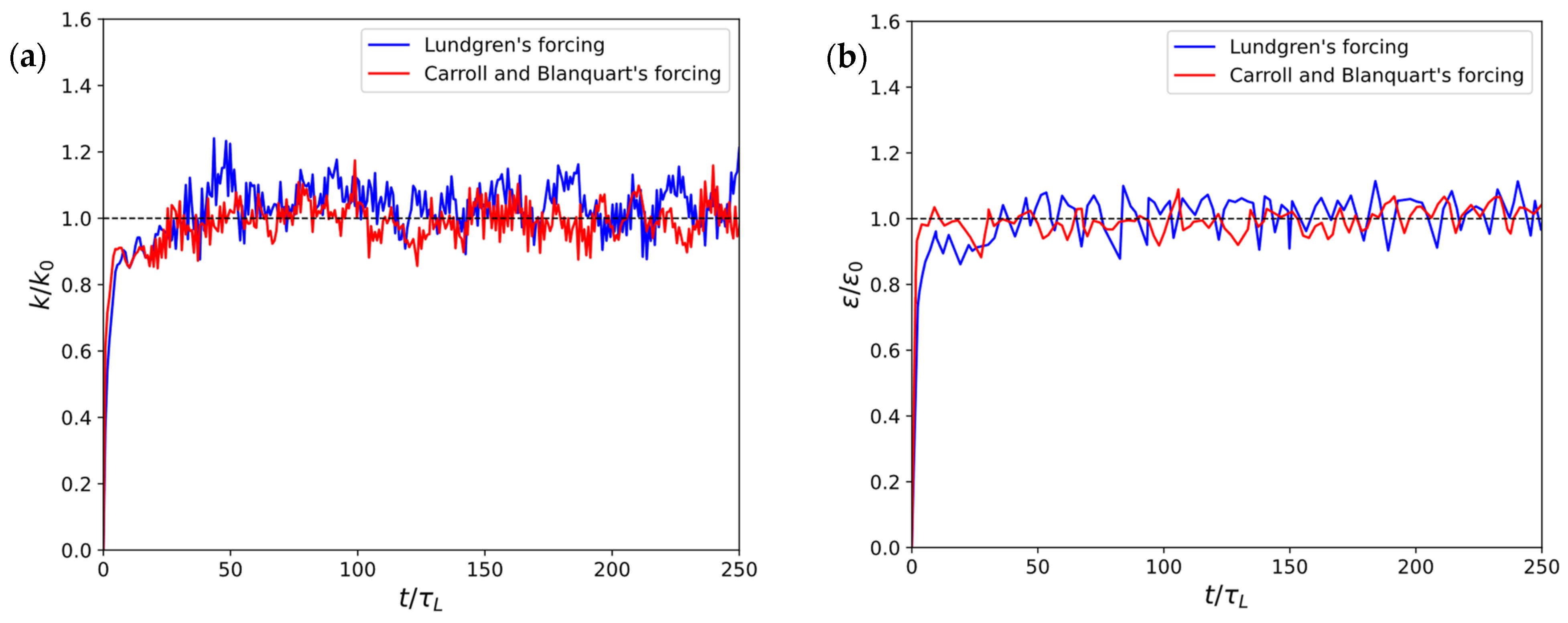
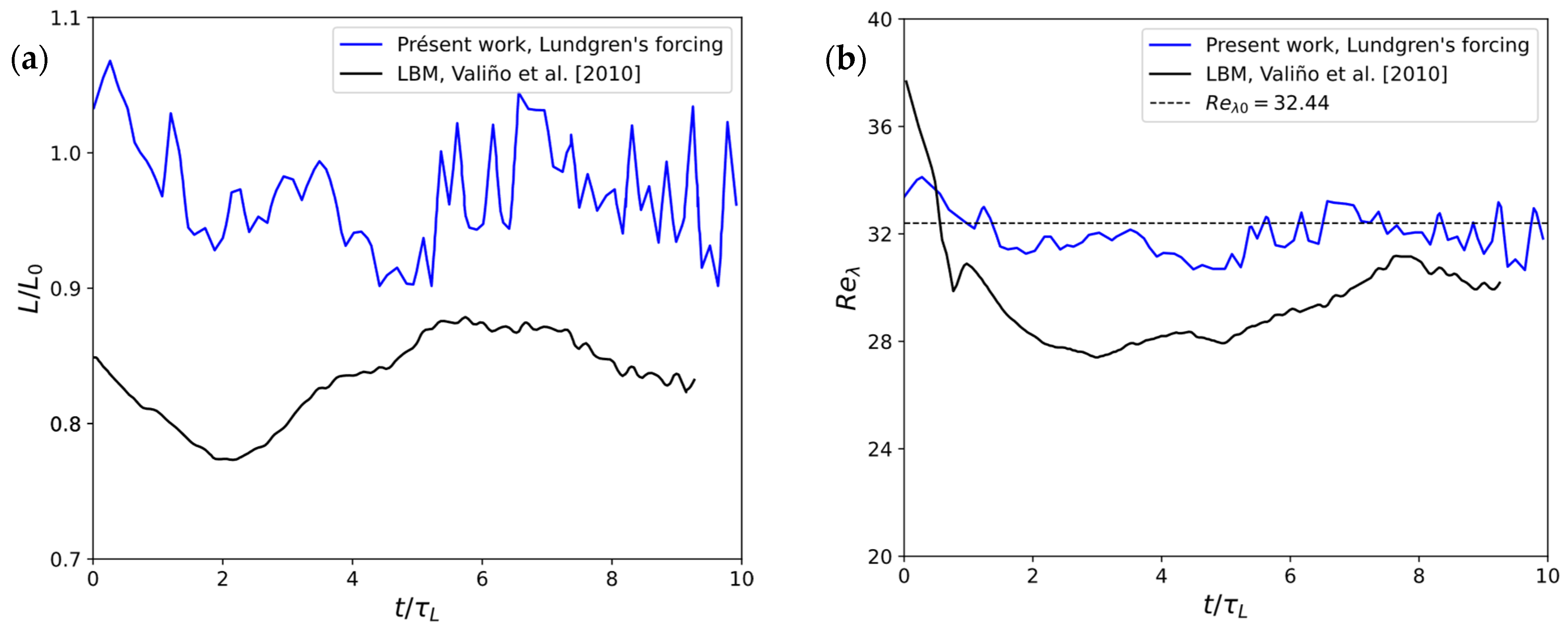
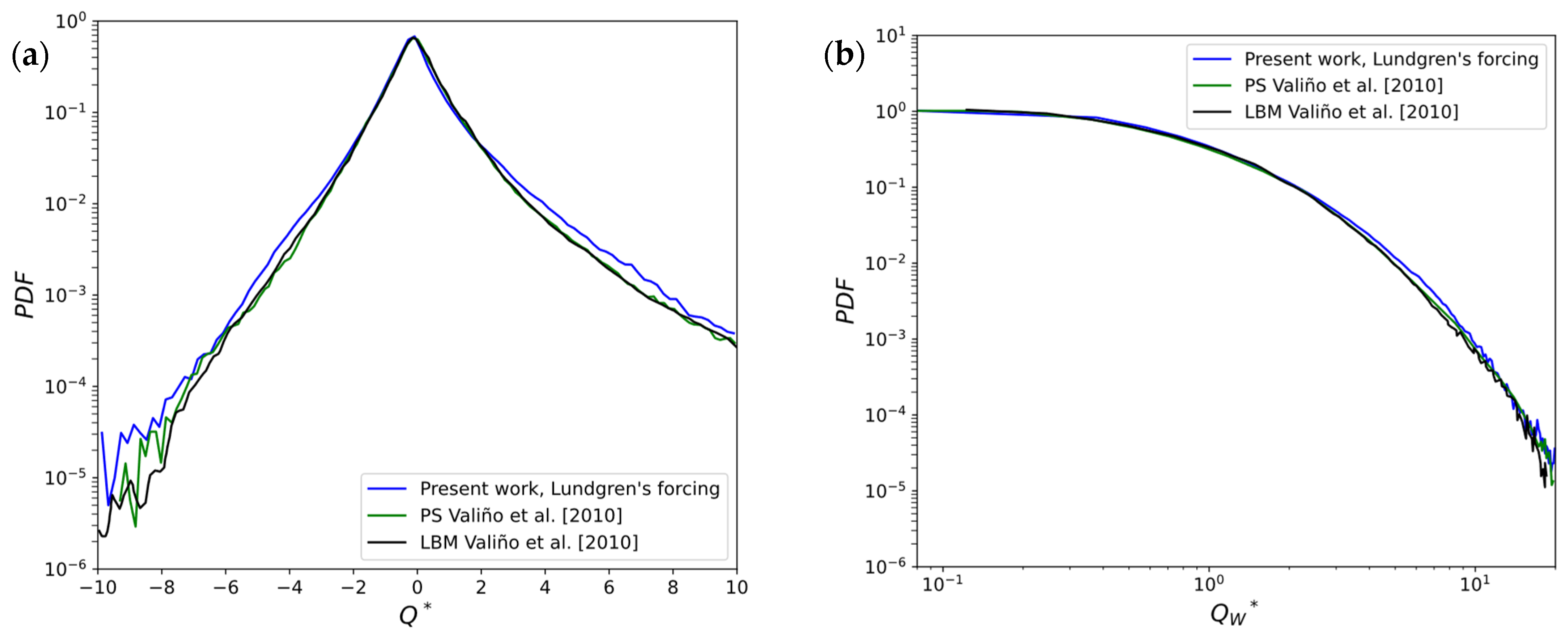
3.1. Turbulent Flow Analysis

In order to verify and compare the performances of the two turbulence forcing approaches described in Section 2.1 (i.e., Lundgren [20] and Carroll and Blanquart [21]), preliminary simulations were initialized with arbitrary velocity fields (of zero mean velocity) far from fully developed turbulent conditions. Figure 1 presents the evolution over time of the turbulent kinetic energy and its dissipation rate computed for the two forcing schemes in such conditions. The time axis is normalized with the eddy turn-over time ${\tau }_L=L_0/u_0$, where $L_0$ is the integral length scale (approximately 20% of the domain size [22]). $k$ is displayed at each time step, whereas ε is displayed with a larger sampling period (${\tau }_L$). As can be seen, both forcing models produce a turbulent flow field with the expected statistics. Both models achieve a very fast statistically steady state around the asymptotic values $k_0$ and ${\epsilon }_0$. However, as already reported in the literature [21], they show different oscillatory characteristics. Lundgren’s forcing exhibits oscillations of slightly larger magnitude, suggesting that it introduces greater variability in turbulent energy levels. Conversely, smaller oscillations of Carroll–Blanquart’s forcing indicate a more controlled energy distribution over time. For these reasons, Carroll–Blanquart’s forcing scheme is used in the study of particle dynamics in Section 3.2.

Simulation results have also been compared to reference simulation results presented by Valiño et al. [28], which were obtained using both LBM with Lundgren’s forcing model and a pseudo-spectral (PS) method with forcing applied in spectral space. For a consistent comparison, Lundgren’s forcing scheme has been used to simulate the same test case as Valiño et al. [28], considering identical flow parameters as those authors.

Figure 2a,b, respectively, present the time evolution of the integral length scale $L={\displaystyle \frac{u^3}{\epsilon }}$ normalized by the target value $L_0=25.6$ and the Taylor microscale Reynolds number ${Re}_{\lambda }$. The figures show a comparison with the results by Valiño et al. [28], obtained using LBM with Lundgren’s forcing model. Our results tend to be overall in better agreement with the target turbulence parameters. Our integral length scale exhibits a rather stable behavior around its target value, with less than 10% fluctuations. In contrast, the results from Valiño et al. [28] show an initial decrease, followed by a gradual increase towards an asymptotic value remaining lower than the target (around 82% of the target). Similarly, our results for ${Re}_{\lambda }$ get very quickly close to the target value ${Re}_{\lambda 0}=32.4$, and show limited oscillations. On the contrary, results by Valiño et al. [28] show a pronounced drop at early times, with a slow recovery over time. These differences in behavior could be due to differences in the LBM used in both works: Valiño et al. [28] have used a D3Q15 lattice with the Bhatnagar–Gross–Krook’s collision operator (BGK) [29], while the present study uses a D3Q18 lattice with Eggels and Somers’s collision operator [18].

As an additional comparison, Figure 3 shows the probability density functions (PDF) of the velocity gradient invariants $Q$ and $Q_W$ extracted from our simulation results and those reported by Valiño et al. Invariant $Q$ is defined as follows:

$$Q={\displaystyle \frac{1}{2}}\left({-(\nabla ·\overrightarrow{u })}^2-\nabla \overrightarrow{u }:{(\nabla \overrightarrow{u })}^T\right)$$

(21)

This invariant reflects both strain and rotational characteristics of the flow, making it useful for identifying the topology of small-scale turbulent structures. The invariant $Q_W$ is the enstrophy density [28]. It is always positive and can be expressed in terms of vorticity $\overrightarrow{{\omega }_f}$ as follows:

$$Q_W={\displaystyle \frac{1}{4}}{\left|\overrightarrow{{\omega }_f}\right|}^2$$

(22)

Figure 3a shows that the PDF of the normalized invariant $Q^{\ast }=Q/<Q_W>$ from our simulation results (blue line) closely follows those deduced from the PS (green line) and LBM (black line) results obtained by Valiño et al. [28] in the central region, where the probability density is the highest. Small deviations between the two works appear when moving toward the extremities of the PDF. As far as the PDF of the normalized invariant ${Q_W}^{\ast }=Q_W/<Q_W>$ is concerned, Figure 3b shows a very good agreement between both works. The three sets of results are almost coincident, displaying a similar decay pattern, with a rapid drop-off as ${Q_W}^{\ast }$ increases. Only very minor discrepancies are noticeable in the very low probability region for large values of ${Q_W}^{\ast }$.

This comparison with the work of Valiño et al. [28] gives us confidence in the correct implementation and accuracy of our LBM solver and in the ability of the linear forcing scheme implemented to reproduce key turbulent flow properties.

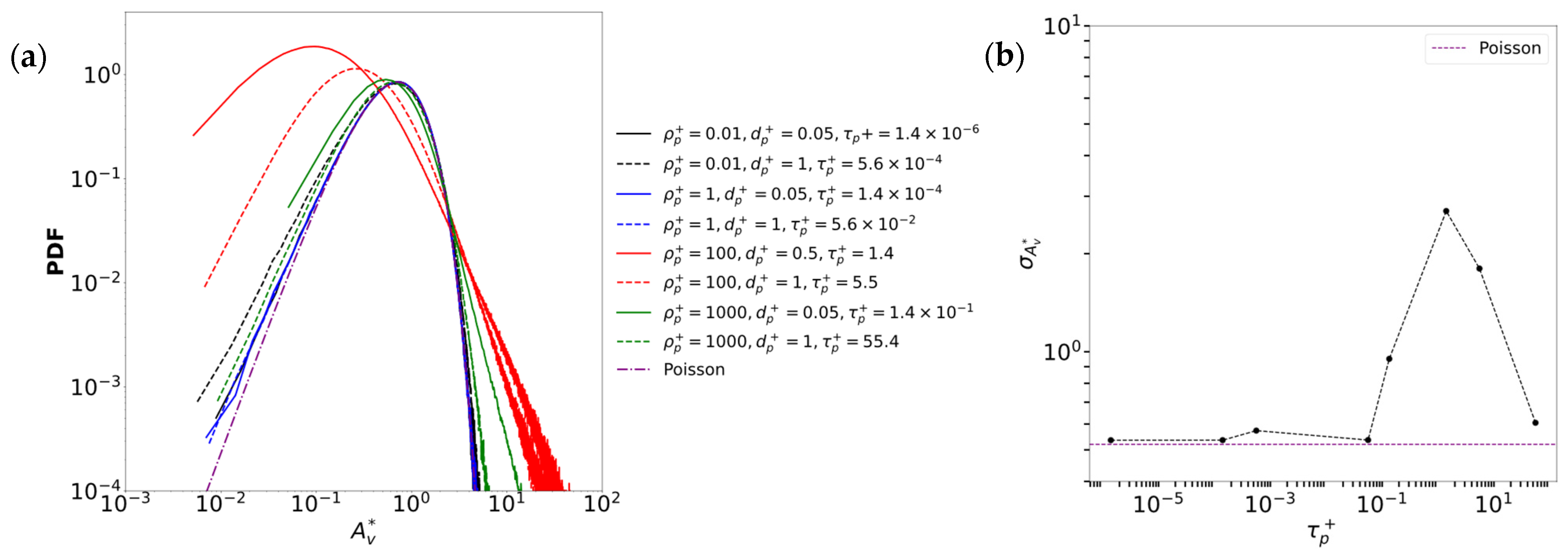
3.2. Cluster Identification

Several methods are commonly used to identify particle clustering in turbulent flows. The clustering index (CI) has been employed in various studies to quantify clustering intensity [30,31], including the review by Shaw et al. [32] on cloud characterization. While simple to compute, this method is highly sensitive to the scale used to define the control volume [30]. The box-counting technique was applied to aerosol clustering by Han et al. [33] and by Baker et al. [34] for coherent clusters in turbulence. This method estimates a fractal dimension but is also highly sensitive to the choice of box size. The radial distribution function (RDF) has been widely employed in both experiments and simulations [16,33,34,35,36,37,38,39], providing a scale-dependent measure of clustering.

The Voronoi diagram approach is an effective method introduced by Monchaux et al. [20], where the PDF of 2D Voronoi cells is analyzed. The standard deviation of these volumes is linked to the clustering intensity and can be compared to theoretical values for random distributions (e.g., 0.52). A standard deviation exceeding this value indicates clustering. This approach eliminates the need for arbitrary criteria, making it particularly suitable for studying particle concentrations [34] and comparing results across studies.

As an illustration of clustering dependence on Stokes number, instantaneous particle distributions and corresponding Voronoi diagrams are presented in Figure 4 for three cases: ${{\tau }_p}^{+}=1.4\times {10}^{-4}$, ${{\tau }_p}^{+}=1.4$, and ${{\tau }_p}^{+}=55.4$. At low Stokes number ${{\tau }_p}^{+}=1.4\times {10}^{-4}$ (left panel), particles are nearly uniformly distributed, leading to Voronoi cells of relatively homogeneous size, reflecting a near-random distribution. At Stokes number ${{\tau }_p}^{+}=1.4$ (middle panel), significant clustering occurs, as evidenced by the presence of small Voronoi cells concentrated in dense regions surrounded by large voids. Finally, at high Stokes number ${{\tau }_p}^{+}=55.4$ (right panel), the particle distribution becomes more dispersed, with reduced clustering and less variation in Voronoi cell sizes.

The qualitative observation that clustering is maximal for Stokes numbers close to 1 is quantitatively supported by the PDFs of the normalized Voronoi cell volumes ${A_v}^{\ast }$, presented in Figure 5 along with their standard deviation ${\sigma }_{{A_v}^{\ast }}$ as a function of the Stokes number. The PDFs, obtained using the method of Monchaux et al. [40], are compared with the Poisson distribution derived from the formula of Ferenc & Néda [41], which serves as a reference for random particle distribution. For small values of the Stokes numbers (from $1.4\times {10}^{-6}$ to $5.5\times {10}^{-2}$), the PDFs closely follow the Poisson distribution, indicating no clustering, which is consistent with tracer-like behavior. This observation is also supported by the low standard deviations of the corresponding PDFs in Figure 5b, which remain close to the theoretical Poisson value of 0.52. As ${{\tau }_p}^{+}$ increases, clustering intensifies, as characterized by the variance of the normalized Voronoi cell PDF, reaching a maximum at ${{\tau }_p}^{+}=1.4$. This is evidenced by a significant shift of the peak value of the PDFs toward smaller Voronoï volumes, accompanied by a broader distribution including larger volumes. This reflects the coexistence of regions of strong particle clustering with regions of large voids, keeping the average concentration constant, since the number of particles and the simulated volume remain unchanged. At such a Stokes number, the standard deviation peaks around 3, highlighting a strong deviation from randomness, well above the Poisson benchmark, characterized by a much lower standard deviation of 0.52 [34,35]. For larger Stokes numbers (e.g., ${{\tau }_p}^{+}=5.5$ and ${{\tau }_p}^{+}=55.4$), the PDF peak shifts back toward larger Voronoï volumes, and the standard deviation decreases significantly. Particles with higher inertia filter short time fluctuations in the flow. They become insensitive to the small scales of turbulence, making them less prone to ejection by small turbulent structures, leading to a more homogeneous spatial distribution.

In summary, the combination of the spatial distributions, PDFs, and standard deviations reveals that particle clustering is most pronounced at intermediate Stokes numbers close to unity. For very small or large Stokes numbers, only little to no clustering happens, with particles either behaving as tracers or being too inertial to concentrate effectively.

To identify regions of high and low concentrations, Figure 6 presents distributions of the strain rate $s^{\ast }$ and rotation rate $r^{\ast }$ in the flow and as seen by particles. The rates are defined as $s^{\ast }=\sqrt{2S_{ij}{S}_{ij}}$, $r^{\ast }=\sqrt{2W_{ij}{W}_{ij}}$, where $S_{ij}={\displaystyle \frac{1}{2}}(\overrightarrow{\nabla }\overrightarrow{u}+{(\overrightarrow{\nabla }\overrightarrow{u})}^T)$ and $W_{ij}={\displaystyle \frac{1}{2}}(\overrightarrow{\nabla }\overrightarrow{u}-{(\overrightarrow{\nabla }\overrightarrow{u})}^T)$. Their values evaluated at the position of particles, respectively denoted ${s_p}^{\ast }$ and ${r_p}^{\ast }$, are reported for the same three Stokes numbers as previously examined (${{\tau }_p}^{+}=1.4\times {10}^{-4}$, ${{\tau }_p}^{+}=1.4$, and ${{\tau }_p}^{+}=55.4$). They provide additional insights into the particle clustering behavior as they reveal distinct particle behaviors depending on particle inertia. At low inertia (${{\tau }_p}^{+}=1.4\times {10}^{-4}$), the curves of $s^{\ast }$ and $r^{\ast }$ overlap with those of ${s_p}^{\ast }$ and ${r_p}^{\ast }$ reflecting a homogeneous particle distribution in the flow. At ${{\tau }_p}^{+}=1.4$, where clustering reaches its maximum, the distributions of $s^{\ast }$ and ${s_p}^{\ast }$ remain close, but the PDF of ${r_p}^{\ast }$ shifts significantly toward smaller values compared to $r^{\ast }$, indicating a preferential accumulation of particles in regions of low vorticity. At high inertia (${{\tau }_p}^{+}=55.4$), the curves of $s^{\ast }$ and $r^{\ast }$ align again with ${s_p}^{\ast }$ and ${r_p}^{\ast }$, signifying that particles remain dispersed without clustering in any specific region. These observations confirm that particle inertia governs clustering dynamics. While low-inertia particles perfectly follow the fluid motion and behave like tracers, particles with a Stokes number close to unity preferentially accumulate in low vorticity regions, confirming that the mechanism driving their clustering is centrifugal ejection from swirling structures. On the other hand, high-inertia particles exhibit reduced sensitivity to turbulent structures and maintain a more uniform distribution.

As a visual confirmation of this interpretation of particle clustering, Figure 7 displays the spatial distribution of particles of ${{\tau }_p}^{+}=1.4$ on top of color maps showing the instantaneous fields $s^{\ast }$ and $r^{\ast }$. It shows that regions of high strain rate in the flow often coincide with regions of high vorticity. However, low vorticity regions seem to be decoupled from strain rate, as previously noted by Jiménez et al. [42] and Wang et al. [43]. Since particles are ejected from high vorticity regions (high $r^{\ast }$), Figure 7 clearly shows that regions of high $r^{\ast }$ are depleted in particles, which preferentially cluster in areas of low $r^{\ast }$, where the strain rate $s^{\ast }$ remains non-negligible. This behavior explains the significant difference between the PDFs of $r^{\ast }$ and ${r_p}^{\ast }$ when clustering happens, while the PDF ${s_p}^{\ast }$ hardly varies with Stokes number and remains close to the one in the flow $s^{\ast }$. This aligns with the findings of Wang et al. [43].

This analysis demonstrates that particle clustering in turbulence is primarily governed by inertia and flow topology. Low-inertia particles behave as ideal tracers, whereas particles with Stokes numbers near unity accumulate preferentially in low-vorticity regions due to centrifugal ejection mechanisms. In contrast, high-inertia particles exhibit a more uniform distribution, reflecting reduced sensitivity to turbulent structures. These observations highlight the pivotal role of inertia and justify a deeper examination of the underlying force balances governing these dynamics.

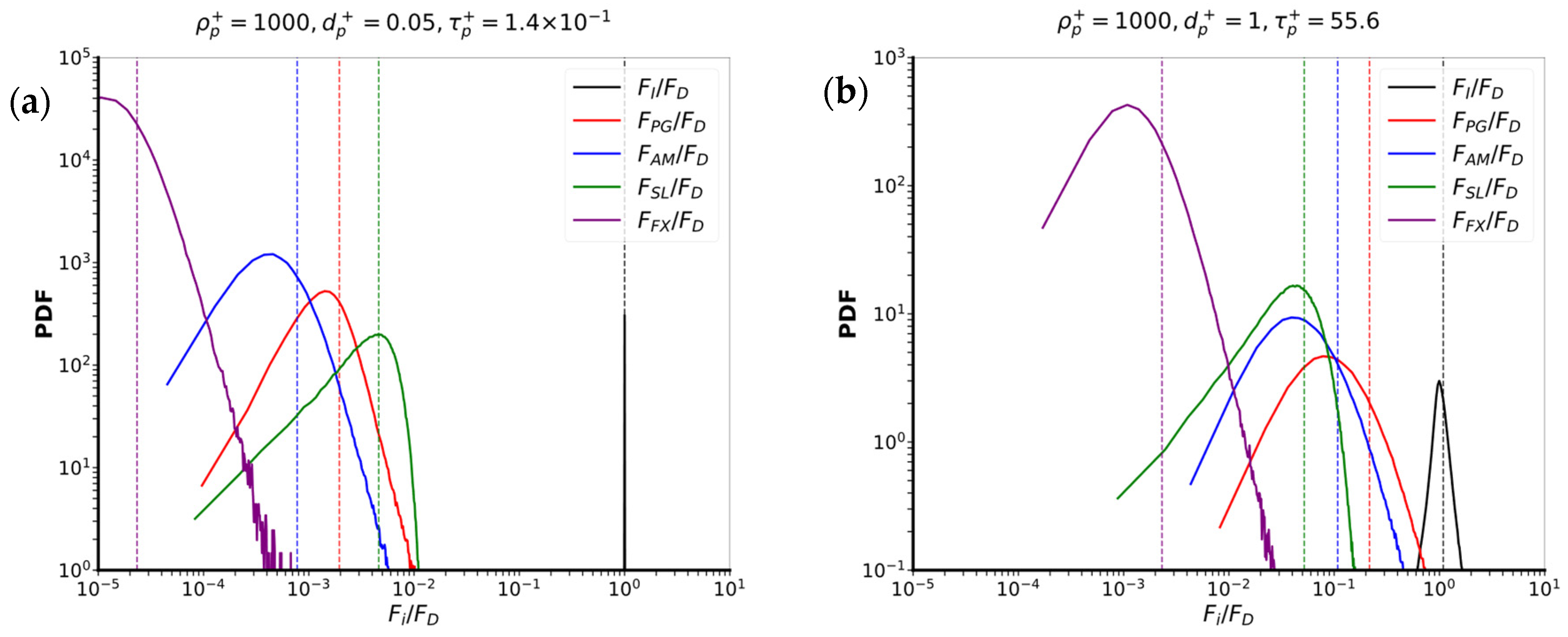
3.3. Relative Importance of the Different Hydrodynamic Contributions Acting on Particles

This section compares the relative contribution of the forces acting on particles. To quantify their contributions, Figure 8, Figure 9 and Figure 10 present the PDFs of their magnitude divided by that of the drag force. Figure 8 shows results for a low particle-to-fluid density ratio (${\rho }_p^{+}=0.01$). For small particles (${d_p}^{+}=0.05$), in Figure 8a, drag force overwhelmingly dominates the particle dynamics, with the contributions of all other forces dependent on particle velocity being significantly lower. This corresponds to conditions for which the particle equation of motion reduces to ${\overrightarrow{F}}_D=\overrightarrow{0}$; thus, particles act as tracers and closely follow the fluid motion. Because the pressure gradient contribution is the only force that does not depend on particle velocity, it is not expressed implicitly in the particle force balance. It is thus constant during the time step of particle motion solving. While its value can be extremely small, ${\overrightarrow{F}}_{PG}=\overrightarrow{\epsilon } \to \overrightarrow{0}$, if drag prevails over all other forces, the numerical solution of the physical behavior ${\overrightarrow{F}}_D=\overrightarrow{0}$ then balances the constant contribution and becomes ${\overrightarrow{F}}_D=\overrightarrow{\epsilon }$. The peak showing ${\overrightarrow{F}}_D={\overrightarrow{F}}_{PG}$, which appears in Figure 8, is thus an artifact of the numerical solver. What Figure 8 actually shows is that drag prevails in the force balance, so such particles always have a velocity equal to that of the fluid and behave as tracers.

Increasing particle size to $d_p^{+}=1$, in Figure 8b, the force balance changes, with all forces then playing a more significant role, except inertia and Faxén’s correction. The biggest contribution comes from the pressure gradient force, which balances the drag force. The added mass and lift forces also have a significant influence on particle dynamics, with an average contribution with respect to the drag of about 40% and 10%, respectively. Note that such an increased importance of the pressure gradient, added mass, and lift forces when increasing the size of the particles is consistent with the fact that these three forces scale with particle volume, while drag scales with diameter in low particulate Reynolds conditions.

Figure 9 shows force ratios in the case of neutrally buoyant particles (${\rho }_p^{+}=1$). Contrary to low-density particles, the results for the smaller particles ($d_p^{+}=0.05$) and for larger particles ($d_p^{+}=1$) are very similar. Indeed, in both cases, pressure gradient and inertia contributions prevail, both being more than 70 times greater than drag. Thus, the particle equation of motion reduces to ${\overrightarrow{F}}_I+{\overrightarrow{F}}_{PG}=\overrightarrow{0}$, which equates particle acceleration and flow acceleration. Such particles thus behave as tracers in the same way as low-density particles, but their dynamics are due to very different underlying mechanisms. Neutrally buoyant particle motion is driven by acceleration terms, even for particles significantly smaller than Kolmogorov’s length scale. Added mass and Faxén’s correction also play a relatively substantial role compared to drag but remain low compared to pressure gradient and inertia contributions.

Figure 10 details the force contributions obtained for dense particles at ${\rho }_p^{+}=1000$. A similar behavior was also observed with a density ratio ${\rho }_p^{+}=100$, which is not reported here. The force balance differs significantly from the ones previously observed for low-density and neutrally buoyant particles. In agreement with typical results reported in the literature [34,35,40] for aerosols, particle dynamics are governed by the balance between inertia and drag, the average ratio of these two forces being around 100%. The pressure gradient, added mass, and lift force contributions are much weaker, while Faxén’s correction is even negligible. Increasing particle size, the pressure gradient, added mass, and lift forces gain more influence, but their contributions remain of second order. As discussed previously, such behavior is consistent with the fact that these three forces scale with particle volume.

In summary, this analysis reveals that low-density, neutrally buoyant, and dense particles experience fundamentally different force balances. Low-density and neutrally buoyant particles both behave as tracers, but for distinct reasons. Low-density particles act as tracers due to the near equality of particle and fluid velocities under dominant drag. Neutrally buoyant particles, on the other hand, follow the fluid because their accelerations align with that of the fluid. This is due to a balance of inertia and pressure gradient forces. Size plays a role in these balances, as larger particles are more impacted by acceleration-related force, while drag has a larger impact on smaller particles. However, in the case of low-density and neutrally buoyant particles, it only slightly changes the overall balance, as the two distinct tracer behaviors (velocity- or acceleration-driven) have been observed on a wide size range from Kolmogorov’s length scale down to particles 20 times smaller. Large particles, close to Kolmogorov’s length scale, with a particle-to-fluid density ratio close to but lower than unity will thus experience a more complex force balance with several forces playing a role but always resulting in tracer behavior in homogeneous isotropic turbulence without gravity.

In contrast, dense particles (aerosols) follow different dynamics, governed by the balance between inertia and drag. These particles can be centrifugally ejected from vortical regions, a clustering mechanism effective only at moderate Stokes numbers. At higher Stokes numbers, their inertia damps the influence of small-scale turbulence, reducing clustering.

4. Conclusions

A lattice Boltzmann method associated with Lagrangian particle tracking has been applied to simulate the dispersion of inertial particles in a forced homogeneous isotropic turbulent flow, considering a wide range of particle-to-fluid density ratios and particle sizes. Simulation results have been used to analyze particle clustering as well as the relative influence of the various forces acting on particles. A comparison of two linear turbulence forcing models, Lundgren’s original method and its modified version by Carroll and Blanquart, has also been presented. The results confirm that the latter provides a more stable energy injection, reducing oscillations in turbulent kinetic energy and leading to faster statistical convergence.

Results on particle clustering show that clustering reaches a maximum at intermediate Stokes number, around unity (${\tau }_p^{+}=1.4$), at which the standard deviation of the normalized Voronoi cell distribution reaches approximately 3, significantly exceeding the Poisson random distribution reference value of 0.52. For low Stokes numbers (${{\tau }_p}^{+}=1.4\times {10}^{-4}$ to $5.6\times {10}^{-2}$), particles behave as tracers, as confirmed by the quantification of the relative impact of force contributions, while at high Stokes numbers (${{\tau }_p}^{+}=55.4$), clustering intensity decreases due to particle inertia preventing them from responding to short-lived turbulent structures. The analysis of velocity gradient invariants confirmed that clustering is primarily driven by particle accumulation in low-vorticity regions, due to their centrifugal ejection from high-vorticity regions when their inertia falls in the right range (Stokes number close to 1).

The main contribution to the dynamics of low-density particles (${{\rho }_p}^{+}=0.01$) is from the drag force in the case of small particle size ($d_p^{+}=0.05$). It remains true in the case of larger particles ($d_p^{+}=1$), but forces scaling with volume (pressure gradient and added mass) also become non-negligible. Neutrally buoyant particles also behave as tracers, but their dynamics are governed by the balance between inertia and pressure gradient, even for small-sized particles down to a twentieth of Kolmogorov’s length scale. The dynamics of high-density particles (${\rho }_p^{+}=1000$) are primarily governed by an equilibrium between inertia and drag. Small particles still behave like tracers due to their low Stokes number. As quantified by the standard deviation of Voronoi cell distribution, clustering appears at a Stokes number value around 0.1, so small dense particles ($d_p^{+}=0.05=0.05$, ${\rho }_p^{+}=1000$, ${{\tau }_p}^{+}=1.4\times {10}^{-1}$) only see little clustering. As particle size increases ($d_p^{+}=1$, ${\rho }_p^{+}=1000$), the influences of pressure gradient, added mass, and lift forces become more significant, although remaining secondary compared to drag and inertia. For all the conditions explored in this study, Faxén’s correction has little impact on particle dynamics.

These findings highlight the complex interplay between turbulence, particle inertia, and the various force contributions acting on particles in turbulent flows. They reveal that particle dynamics are governed by fundamentally different force balances depending on particle density and size, even among particles that behave as tracers within the turbulent flow considered here. For low-density and neutrally buoyant particles, tracer-like behavior emerges through distinct mechanisms, one driven by the near equality of velocities, the other by a balance of accelerations. Dense particles exhibit inertia-dominated dynamics with preferential ejection from vortical structures at moderate Stokes numbers. These insights contribute to a more comprehensive understanding of turbulence-driven particle dynamics and underline the importance of accurately modeling non-negligible forces such as pressure gradient, added mass, and lift. Future work will focus on extending this analysis to higher Reynolds number flows. This would increase the scale separation between the largest and smallest turbulent structures, and, given that the forcing model employed is conditioned by the size of the domain, it would require enlarging the computational domain accordingly, thus significantly increasing the computational cost. Additionally, incorporating history force would refine the description of unsteady effects in particle motion. However, doing so would necessitate the storage and retrieval of the particle velocity history over time, which increases both memory requirements and numerical cost. Optimized numerical strategies for modeling this force will therefore be necessary. Another important direction would be to investigate particle dynamics in anisotropic and inhomogeneous turbulent flows, which are more representative of real-world configurations such as wall-bounded turbulence, jets, or environmental flows, where force balances and preferential concentration mechanisms could differ substantially from the homogeneous isotropic case explored here. In such configurations, the behavior of the linear forcing model adopted here remains uncertain and may not perform reliably.

Overall, these extensions involve non-trivial theoretical and numerical challenges that will be the subject of future investigations.

References

1. Guha, A. Transport and Deposition of Particles in Turbulent and Laminar Flow. Annu. Rev. Fluid Mech. 2008, 40, 311–341. [Google Scholar] [CrossRef]
2. Domingo, P.; Vervisch, L.; Réveillon, J. DNS analysis of partially premixed combustion in spray and gaseous turbulent flame-bases stabilized in hot air. Combust. Flame 2005, 140, 172–195. [Google Scholar] [CrossRef]
3. Eskin, D.; Ratulowski, J.; Akbarzadeh, K.; Andersen, S. Modeling of asphaltene deposition in a production tubing. AIChE J. 2012, 58, 2936–2948. [Google Scholar] [CrossRef]
4. Bellot, J.-P.; Kroll-Rabotin, J.-S.; Gisselbrecht, M.; Joishi, M.; Saxena, A.; Sanders, S.; Jardy, A. Toward Better Control of Inclusion Cleanliness in a Gas Stirred Ladle Using Multiscale Numerical Modeling. Materials 2018, 11, 1179. [Google Scholar] [CrossRef]
5. Huai, W.; Li, S.; Katul, G.G.; Liu, M.; Yang, Z. Flow dynamics and sediment transport in vegetated rivers: A review. J. Hydrodyn. 2021, 33, 400–420. [Google Scholar] [CrossRef]
6. Squires, K.D.; Eaton, J.K. Preferential concentration of particles by turbulence. Phys. Fluids A Fluid Dyn. 1991, 3, 1169–1178. [Google Scholar] [CrossRef]
7. Eaton, J.K.; Fessler, J.R. Preferential concentration of particles by turbulence. Int. J. Multiph. Flow 1994, 20, 169–209. [Google Scholar] [CrossRef]
8. Wang, L.-P.; Maxey, M.R. Settling velocity and concentration distribution of heavy particles in homogeneous isotropic turbulence. J. Fluid Mech. 1993, 256, 27–68. [Google Scholar] [CrossRef]
9. Aliseda, A.; Cartellier, A.; Hainaux, F.; Lasheras, J.C. Effect of preferential concentration on the settling velocity of heavy particles in homogeneous isotropic turbulence. J. Fluid Mech. 2002, 468, 77–105. [Google Scholar] [CrossRef]
10. Ireland, P.J.; Bragg, A.D.; Collins, L.R. The effect of Reynolds number on inertial particle dynamics in isotropic turbulence. Part 1. Simulations without gravitational effects. J. Fluid Mech. 2016, 796, 617–658. [Google Scholar] [CrossRef]
11. Brandt, L.; Coletti, F. Particle-Laden Turbulence: Progress and Perspectives. Annu. Rev. Fluid Mech. 2022, 54, 159–189. [Google Scholar] [CrossRef]
12. Maxey, M.R.; Riley, J.J. Equation of motion for a small rigid sphere in a nonuniform flow. Phys. Fluids 1983, 26, 883–889. [Google Scholar] [CrossRef]
13. Armenio, V.; Fiorotto, V. The importance of the forces acting on particles in turbulent flows. Phys. Fluids 2001, 13, 2437–2440. [Google Scholar] [CrossRef]
14. Elghobashi, S.; Truesdell, G.C. Direct simulation of particle dispersion in a decaying isotropic turbulence. J. Fluid Mech. 1992, 242, 655–700. [Google Scholar] [CrossRef]
15. Daitche, A. On the role of the history force for inertial particles in turbulence. J. Fluid Mech. 2015, 782, 567–593. [Google Scholar] [CrossRef]
16. Olivieri, S.; Picano, F.; Sardina, G.; Iudicone, D.; Brandt, L. The effect of the Basset history force on particle clustering in homogeneous and isotropic turbulence. Phys. Fluids 2014, 26, 041704. [Google Scholar] [CrossRef]
17. Yokojima, S.; Shimada, Y.; Mukaiyama, K. A further study of history force effect on particle clustering in turbulence. Eur. J. Mech.-B/Fluids 2024, 103, 11–24. [Google Scholar] [CrossRef]
18. Eggels, J.G.M.; Somers, J.A. Numerical simulation of free convective flow using the lattice-Boltzmann scheme. Int. J. Heat Fluid Flow 1995, 16, 357–364. [Google Scholar] [CrossRef]
19. Sungkorn, R.; Derksen, J.J. Simulations of dilute sedimenting suspensions at finite-particle Reynolds numbers. Phys. Fluids 2012, 24, 123303. [Google Scholar] [CrossRef]
20. Lundgren, T.S. Linearly forced isotropic turbulence. Annu. Res. Briefs 2003, 461–473. [Google Scholar]
21. Carroll, P.L.; Blanquart, G. A proposed modification to Lundgren’s physical space velocity forcing method for isotropic turbulence. Phys. Fluids 2013, 25, 105114. [Google Scholar] [CrossRef]
22. Rosales, C.; Meneveau, C. Linear forcing in numerical simulations of isotropic turbulence: Physical space implementations and convergence properties. Phys. Fluids 2005, 17, 095106. [Google Scholar] [CrossRef]
23. Schiller, L.; Naumann, A. A drag coefficient correlation. Z. Ver. Dtsch. Ing. 1933, 77, 318–320. [Google Scholar]
24. Saffman, P.G. The lift on a small sphere in a slow shear flow. J. Fluid Mech. 1965, 22, 385–400. [Google Scholar] [CrossRef]
25. Mei, R. An approximate expression for the shear lift force on a spherical particle at finite reynolds number. Int. J. Multiph. Flow 1992, 18, 145–147. [Google Scholar] [CrossRef]
26. Taylor, G.I. The forces on a body placed in a curved or converging stream of fluid. Proc. R. Soc. Lond. Ser. A Contain. Pap. Math. Phys. Character 1928, 120, 260–283. [Google Scholar] [CrossRef]
27. Magnaudet, J.; Rivero, M.; Fabre, J. Accelerated flows past a rigid sphere or a spherical bubble. Part 1. Steady straining flow. J. Fluid Mech. 1995, 284, 97–135. [Google Scholar] [CrossRef]
28. Valiño, L.; Martín, J.; Házi, G. Dynamics of Isotropic Homogeneous Turbulence with Linear Forcing Using a Lattice Boltzmann Method. Flow Turbul. Combust. 2010, 84, 219–237. [Google Scholar] [CrossRef]
29. Bhatnagar, P.L.; Gross, E.P.; Krook, M. A Model for Collision Processes in Gases. I. Small Amplitude Processes in Charged and Neutral One-Component Systems. Phys. Rev. 1954, 94, 511–525. [Google Scholar] [CrossRef]
30. Monchaux, R.; Bourgoin, M.; Cartellier, A. Analyzing preferential concentration and clustering of inertial particles in turbulence. Int. J. Multiph. Flow 2012, 40, 1–18. [Google Scholar] [CrossRef]
31. Baker, B.; Lawson, R.P. Analysis of Tools Used to Quantify Droplet Clustering in Clouds. J. Atmos. Sci. 2010, 67, 3355–3367. [Google Scholar] [CrossRef]
32. Shaw, R.A.; Kostinski, A.B.; Larsen, M.L. Towards quantifying droplet clustering in clouds. Q. J. R. Meteorol. Soc. 2002, 128, 1043–1057. [Google Scholar] [CrossRef]
33. Han, K.; Lee, H.; Hwang, W. Pseudo real-time continuous measurements of particle preferential concentration in homogeneous isotropic turbulence. Exp. Therm. Fluid Sci. 2020, 112, 109968. [Google Scholar] [CrossRef]
34. Baker, L.; Frankel, A.; Mani, A.; Coletti, F. Coherent clusters of inertial particles in homogeneous turbulence. J. Fluid Mech. 2017, 833, 364–398. [Google Scholar] [CrossRef]
35. Wood, A.M.; Hwang, W.; Eaton, J.K. Preferential concentration of particles in homogeneous and isotropic turbulence. Int. J. Multiph. Flow 2005, 31, 1220–1230. [Google Scholar] [CrossRef]
36. Petersen, A.J.; Baker, L.; Coletti, F. Experimental study of inertial particles clustering and settling in homogeneous turbulence. J. Fluid Mech. 2019, 864, 925–970. [Google Scholar] [CrossRef]
37. Shen, J.; Lu, Z.; Wang, L.-P.; Peng, C. Influence of particle-fluid density ratio on the dynamics of finite-size particles in homogeneous isotropic turbulent flows. Phys. Rev. E 2021, 104, 025109. [Google Scholar] [CrossRef]
38. Bec, J.; Gustavsson, K.; Mehlig, B. Statistical Models for the Dynamics of Heavy Particles in Turbulence. Annu. Rev. Fluid Mech. 2024, 56, 189–213. [Google Scholar] [CrossRef]
39. Ariki, T.; Yoshida, K.; Matsuda, K.; Yoshimatsu, K. Scale-similar clustering of heavy particles in the inertial range of turbulence. Phys. Rev. E 2018, 97, 033109. [Google Scholar] [CrossRef]
40. Monchaux, R.; Bourgoin, M.; Cartellier, A. Preferential concentration of heavy particles: A Voronoï analysis. Phys. Fluids 2010, 22, 103304. [Google Scholar] [CrossRef]
41. Ferenc, J.-S.; Néda, Z. On the size distribution of Poisson Voronoi cells. Phys. A Stat. Mech. Its Appl. 2007, 385, 518–526. [Google Scholar] [CrossRef]
42. Jiménez, J.; Wray, A.A.; Saffman, P.G.; Rogallo, R.S. The structure of intense vorticity in isotropic turbulence. J. Fluid Mech. 1993, 255, 65–90. [Google Scholar] [CrossRef]
43. Wang, X.; Wan, M.; Yang, Y.; Wang, L.-P.; Chen, S. Reynolds number dependence of heavy particles clustering in homogeneous isotropic turbulence. Phys. Rev. Fluids 2020, 5, 124603. [Google Scholar] [CrossRef]
Figure 1. Time evolution of (a) the normalized turbulent kinetic energy k / k 0 and (b) the normalized dissipation rate ε / ε 0 . Time axis is scaled by the turn-over time of large eddies τ L .
Fluids 10 00201 g001
Figure 2. Time evolution of (a) L / L 0 and (b) R e λ . Time is normalized by the large-eddy turn-over time. Comparison with the numerical results from Valiño et al. [28].
Fluids 10 00201 g002
Figure 3. (a) PDF of the invariant Q and (b) of the invariant Q W , both normalized by the mean enstrophy < Q W > . Comparison with the numerical results from Valiño et al. [28].
Fluids 10 00201 g003
Figure 4. Two-dimensional Voronoï tessellation of a slice with a thickness of 3 η for increasing Stokes numbers τ p + = 1.4 × 10 4 (left), τ p + = 1.4 (middle), and τ p + = 55.4 (right).
Fluids 10 00201 g004
Figure 5. (a) PDFs of Voronoï cell volumes, normalized by the mean cell volume for various particles, compared with the Poisson distribution. (b) Standard deviation of normalized Voronoï volume distributions as a function of Stokes number.
Fluids 10 00201 g005
Figure 6. PDFs of the normalized (a) strain rate in the flow s and at particle positions s p , and (b) rotation rate in the flow r and at particle positions r p , for the Stokes numbers ( τ p + = 1.4 × 10 4 , 1.4 , and 55.4 ).
Fluids 10 00201 g006
Figure 7. Instantaneous particle positions for τ p + = 1.4 overlaying color maps of the normalized (a) strain rate s and (b) rotation rate r .
Fluids 10 00201 g007
Figure 8. Probability density functions of the ratio of the magnitude of each force to the magnitude of the drag force. (a) case 1: ρ p + = 0.01 ,   d p + = 0.05 ,   τ p + = 1.4 × 1 0 6 , (b) case 2: ρ p + = 0.01 ,   d p + = 1 , τ p + = 5.6 × 1 0 4 . The vertical lines show the positions of the average.
Fluids 10 00201 g008
Figure 9. Probability density functions of the ratio of the magnitude of each force to the magnitude of the drag force. (a) case 3: ρ p + = 1 ,   d p + = 0.05 ,   τ p + = 1.4 × 1 0 4 , (b) case 4: ρ p + = 1 ,   d p + = 1 ,   τ p + = 5.6 × 1 0 2 . The vertical lines show the positions of the average.
Fluids 10 00201 g009
Figure 10. Probability density functions of the ratio of the magnitude of each force to the magnitude of the drag force. (a) case 7: ρ p + = 1000 ,   d p + = 0.05 ,   τ p + = 1.4 × 1 0 1 ; (b) case 8: ρ p + = 1000 ,   d p + = 1 ,   τ p + = 55.6 . The vertical lines show the positions of the average.
Fluids 10 00201 g010