Abstract
Presented in this work is a harmonic balance (HB)-based pseudo-time code-coupling approach applied to a one-degree-of-freedom vortex-induced vibration (VIV) problem of a circular cylinder in a low-Reynolds-number laminar flow regime. Unlike physical time coupling used in traditional time-accurate methods, this novel approach updates both of the fluid and structure fields by integrating respective HB forms of governing equations in pseudo-time, and then couples the two fields in pseudo-time using a partitioned approach. A separate procedure is adopted to determine the VIV frequency at every code-coupling iteration, which enables the simultaneous convergence of variables of both fields in a single run of the solver. For the cases considered here, lock-in vibrations are predicted over a range of Reynolds numbers, inside and outside the resonant range. The results are verified by a time-accurate method and also validated against earlier experimental data, demonstrating the efficiency and robustness of the pseudo-time code-coupling approach.
1. Introduction
For certain flow conditions, laminar flow around a blunt body results in vortex shedding in the downstream, which induces unsteady fluid-driven loads that exert back on the elastic body, and force the body to vibrate if the structural damping of the system is relatively low. Such a self-excited fluid–structure interaction (FSI) phenomenon is also referred to as vortex-induced-vibration (VIV) [1,2,3,4,5]. Usually, a VIV can be interpreted as lock-in if the vortex shedding frequency coincides with the frequency of the oscillating body, or as non-lock-in otherwise. In this field, one of the most extensively used benchmark cases is the one-degree-of-freedom (DOF) VIV system of Anagnostopoulos and Bearman [6], who investigated cylinder VIV experimentally for a range of Reynolds numbers in the laminar flow regime. Traditionally, this case has been studied numerically using time-accurate approaches in which the fluid and structural fields are coupled and synchronized in physical time [7,8,9,10,11,12,13,14,15,16,17,18]. In order to ensure an acceptable accuracy, the physical time step is usually taken to be small and should have the same value for both the fluid and structural fields. Although this approach is robust and straightforward, time-accurate solvers tend to be computationally costly since long transients need to be resolved before the desired periodic/modulation state is reached.
For time-periodic VIV problems, one of the efficient alternatives to the time-accurate approach is the Fourier-based harmonic balance (HB) method (also known as the time-spectral method) introduced in the field of computational fluid dynamics about two decades ago [19,20]. This technique has been shown to accurately model strong nonlinearities in the flowfield, while offering significant computational savings. In this approach, one models the complex nonlinear flowfield at a number of equally spaced sub-time levels that span a single period of the unsteady response. The solutions at these individual sub-time levels are coupled through a Fourier-based time-spectral operator that approximates the physical time derivative term in the governing equations. As a result, the problem is converted into a mathematically steady form, which can be solved efficiently with the addition of a pseudo-time term. By circumventing long initial transients of the time-accurate response and dealing directly with the periodic pattern, the HB method has been proven to be orders of magnitude more efficient compared to traditional time-accurate methods [21,22,23,24,25].
The pioneering application of the HB technique to VIV problems dates back to the work of Carlson et al. [26], in which the HB/LCO method originally developed by Thomas et al. [27] for solving limit-cycle-oscillation (LCO) problems was applied to model the above-mentioned one-DOF VIV system [6]. This work was performed as an initial step towards modeling non-synchronous vibrations (NSV) in turbomachinery [28,29,30,31,32,33]. In this approach, a solution vector consisting of structural amplitudes and the VIV frequency is solved iteratively using the Newton–Raphson method, requiring repeated HB flow solver runs to calculate the terms in the Jacobian matrix of the Newton’s solver for each code-coupling iteration. As such, the computational cost scales linearly with the number of structural DOFs. This means that for a complex structural system with many degrees of freedom, the HB/LCO method may become expensive. In order to work around this issue, Thomas and Dowel [34] recently proposed an improvement to the HB/LCO method, in which a fixed-point iteration [35] is used and both fluid and structural solvers are converged simultaneously, making the computational cost of the VIV analysis independent of the number of structural DOF. Berci and Dimitriadis [36] implemented an HB-based approach similar to the HB/LCO method, which was augmented with a multiple-time-scale solver to capture the transient response of dynamic systems. Readers are referred to the work of Yao and Jaiman [37] and the work of Nardini et al. [38] for a similar approach based on a fixed-point iteration, which is not detailed here for brevity.
Besides the HB/LCO method, various HB-based code-coupling schemes have been developed in the literature. A monolithic method similar to the HB/LCO approach was developed by He et al. [39,40,41], who assembled the dependent variables of both the fluid and structure fields into one global unknown vector and solved the resultant system using a Newton–Krylov method. Maljaars et al. [42] also advocated a similar Krylov subspace method to solve Fourier-transformed equations of periodic FSI problems, except that the two fields were coupled in a partitioned fashion. Different from the methods mentioned above, Ekici and Hall [43] proposed the so-called One-shot method to solve the self-excited LCO response in turbomachinery. In this approach, both fluid and structural solvers were cast into a mathematically steady HB form and were solved using pseudo-time integration. The two solvers are then coupled using a partitioned approach in pseudo-time, in contrast to the physical time used in traditional time-accurate methods. At every FSI iteration, the value of the LCO frequency is updated by an optimization procedure designed to minimize the residual of the structural solver. Ultimately, this technique allows for the use of different pseudo-time step sizes and different integration schemes for each field, and both solvers are converged simultaneously in a single run. This flexibility is the biggest advantage of this technique, which ensures DOF-independent computational cost. Following the earlier work of Ekici and Hall [43], the One-shot approach has been further developed for solving various periodic FSI problems by Li and Ekici [44,45,46,47]. In all of these studies, the One-shot method has been shown to be very efficient and robust.
This work aims to extend the application of the One-shot method into modeling VIV problems, and the one-DOF benchmark VIV system of Anagnostopoulos and Bearman [6] is studied. To the authors’ best knowledge, this is the first time that the One-shot pseudo-time code-coupling approach has been applied to VIV-type FSI problems. Note that the identification of a lock-in VIV boundary in terms of structural parameters [48,49] is not considered here, and this work focuses on predicting possible lock-in VIV conditions by the One-shot method over a range of Reynolds numbers, inside and outside the resonant range. Particularly, the transition of vibration from a non-lock-in state to a lock-in state outside the resonant range is unveiled and analyzed. Almost all time-accurate analyses reported in the literature that investigated this interesting FSI problem appear to have stopped the time-marching simulations prematurely, which was discovered and confirmed by the use of an HB-based One-shot approach. The rest of this paper is organized as follows: the governing equations of the one-DOF VIV system and the computational fluid dynamics (CFD) solver are presented first. Then, the pseudo-time code-coupling approach of the One-shot solver is detailed. Following this, the HB-CFD solver is validated for vortex shedding problems associated with a circular cylinder. After that, the VIV results of the One-shot approach are presented with discussions of different VIV phenomena, and the efficiency and the robustness of the One-shot approach are also demonstrated.
2. Materials and Methods
2.1. Governing Equations
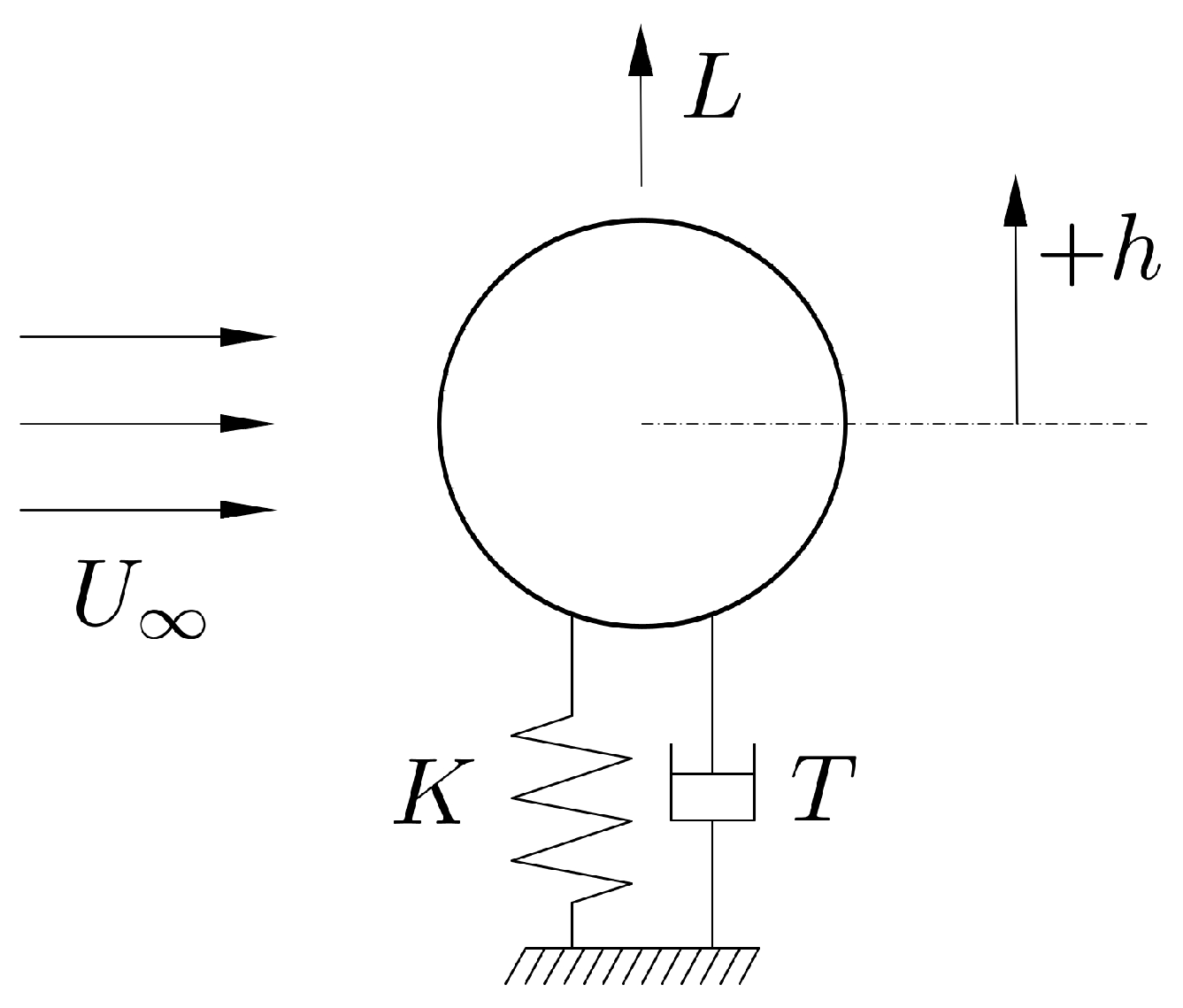
2.1.1. The One-DOF VIV Model
The one-DOF VIV system of Anagnostopoulos and Bearman [6] can be modeled as a cylinder in two-dimensional laminar cross-flow undergoing transverse oscillations, as depicted in Figure 1.
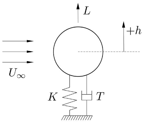
Figure 1.
The one-DOF VIV model of a cylinder in two-dimensional laminar cross-flow.
With the assumption of constant structural damping and linear elasticity, the structural dynamics of the above VIV system are governed by a simple differential equation given by
where m is the mass of the cylinder, T is the structural damping coefficient, K is the spring stiffness, is the freestream dynamic pressure, D is the cylinder diameter, s is the cylinder span, is the cylinder lift coefficient, and h is the transverse displacement of the cylinder. Following the work of Carlson et al. [26], Equation (1) can be nondimensionalized (by taking the cylinder diameter D as the reference length) and rewritten as
One common practice for solving the problem defined by Equation (2) is to recast the equation into the state-space form as
where
2.1.2. The Unsteady Flow Solver
In order to obtain accurate solutions of cylinder vibrations governed by Equation (4), a flow solver that can properly resolve the vortex shedding and the generalized force, , is required. In this work, we use an in-house CFD solver that models laminar Navier–Stokes equations. In two-dimensional Cartesian coordinates, the strong conservation form of these equations is given by
where is the vector of conservation variables, and and are the flux vectors, which are all defined as
Here, and are the x and y components of the velocity of the unsteady grid that accounts for the motion of the cylinder. In the CFD solver, the non-dimensional form of the above equations are implemented.
The computational domain surrounding the cylinder is discretized by a structured and body-fitted O-type mesh. The governing equations (Equation (5)) are discretized using a cell-vertex finite volume scheme [50,51] in which the convective and viscous fluxes are evaluated using a central scheme. An artificial dissipation term, originally developed by Jameson et al. [52], is added to inviscid fluxes to avoid odd-even decoupling. On the cylinder surface, adiabatic and no-slip conditions for viscous flows are imposed. At the far-field, one-dimensional characteristic boundary conditions are used, and along the O-grid branch cut flow, continuity is ensured by the use of periodic boundary conditions. The resulting semi-discrete equations are integrated using a multi-stage Runge–Kutta scheme [52]. In addition, local time stepping [51] and multigrid [53] techniques are incorporated to accelerate numerical convergence. Note that a compressible flow solver is used here to couple with the structural solver to resolve the flow fields of cylinder VIV at low Reynolds numbers, which are essentially incompressible, and our numerical experiments reveal that a Mach number of 0.2 is sufficiently small, allowing the use of a compressible solver to model incompressible flows. Earlier studies have also reported a similar finding [24,46,54]. For the cylinder case studied here, a standalone incompressible flow solver based on the artificial compressibility method of Chorin [55] is also employed to validate the compressible solver, which will be presented later in Section 3.1.
2.2. The One-Shot Method
As introduced in the earlier sections, the essence of the One-shot method is the HB technique, which reduces the order in the physical time domain and converts time-periodic problems into mathematically steady ones. Based on this, fluid and structural domains can be coupled in pseudo-time instead of physical time. Before discussing the One-shot code-coupling approach, the application of the HB technique to the flow and structural governing equations is explained in what follows.
2.2.1. The High-Dimensional Harmonic Balance Technique
With the assumption that the flow field is periodic in time and that the cylinder vibration is stable (finite amplitude vibration at a single frequency and its harmonics), the dependent variables in Equations (4) and (5) can be approximated as a truncated Fourier series up to a prescribed number of harmonics, N. As such, the vector of conservation variables can be written as
where , is the fundamental frequency of unsteadiness, and and are the spatially varying Fourier coefficients of the conservation variables. Rewriting Equation (6) in matrix-vector form, one gets
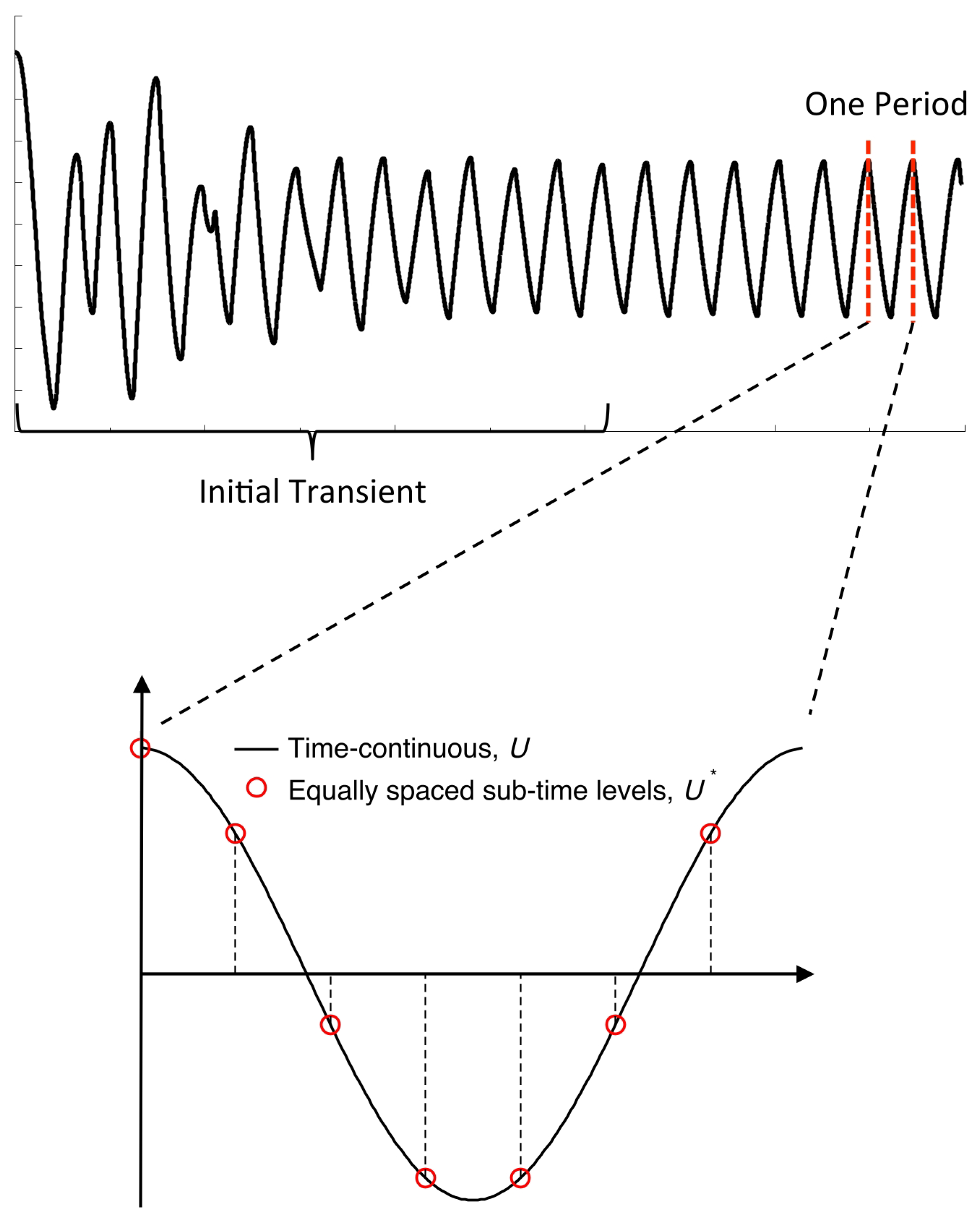
where is the inverse discrete Fourier transformation matrix. Clearly, the Fourier series is truncated in a way that the flow variables, , are computed and stored at equally spaced sub-time levels over a single period. For example, seven sub-time levels are used when three harmonics are retained in the analysis, as demonstrated in Figure 2.
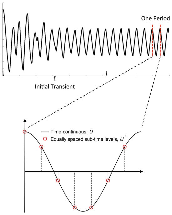
Figure 2.
The HB technique avoids the initial transient and deals directly with the periodic pattern by solving the instantaneous solutions at equally spaced sub-time levels covering one period.
Conversely, the Fourier series coefficients can be determined from solutions stored at sub-time levels by a discrete Fourier transformation, , so that
Note that the transformation matrix, , and its inverse, , are square matrices. Next, Equation (5) is written at all sub-time levels simultaneously, so that
where, for example, is the vector of x fluxes evaluated at . For two-dimensional laminar flows, Equation (5) contains four equations; therefore, Equation (8) will have equations that are coupled through the time derivative term, which is approximated by the pseudo-spectral operator . Therefore, Equation (8) becomes
Note that the excitation frequency in the above equation is written in a reduced form, , since a non-dimensional CFD solver is used. Note also that the matrix in the pseudo-spectral operator is not dependent on the value of the frequency, and its terms are constant for a certain number of harmonics retained in the model. For example, if two harmonics are retained to model time-periodic problems, the matrix is given by:
As can be seen, Equation (9) has no time-derivative term, which makes it mathematically steady. To simplify the solution of these nonlinear equations, a common approach is to introduce a pseudo-time derivative term to make the system hyperbolic in pseudo-time, and rapidly march the solution to steady state in pseudo-time using conventional CFD schemes. With the inclusion of this term, Equation (9) takes the following form:
Similarly, the governing equation modeling the structural dynamics (Equation (4)) can be rewritten in the HB form and augmented by a pseudo-time term so that
It is worth mentioning that when solving the HB equations in pseudo-time, the physical time step becomes essentially the time interval between two successive sub-time levels, as shown in Figure 2. This step size is apparently much larger than that of a classical dual-time stepping approach, which would require very small physical time steps to ensure the stability and the accuracy of the unsteady solution. Note that the two HB equations (Equations (10) and (11)) share the same frequency, , since the VIV responses studied in this work are assumed to lock-in. In addition, the frequency in its reduced form, , is used, which is defined based on the angular frequency. However, as is commonly done for flows with vortex shedding, the non-dimensional regular frequency, , is used later in presenting the results of VIV cases studied in this work, and it can be calculated from directly through . As a side note, for the remainder of this work, the superscript * in Equations (10) and (11) will be dropped for simplicity.
2.2.2. Fluid–Structure Code-Coupling in Pseudo-Time
The code-coupling of the One-shot method in pseudo-time is illustrated in Figure 3, which is similar to the conventional serial staggered (CSS) scheme widely used in time-accurate approaches.
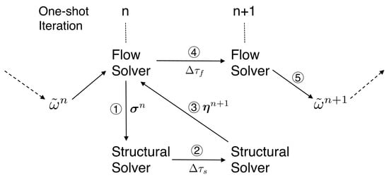
Figure 3.
One iteration of One-shot pseudo-time code-coupling approach, steps of which are indicated by the numbers in circles.
It must be noted that different pseudo-time step sizes ( and ) for the fluid and structure fields are used to emphasize the fact that two fields need not be advanced with the same pseudo-time (or integration technique) in the One-shot approach—a significant advantage of the current method over existing FSI solution techniques. In addition, although the CSS-type scheme has first-order time accuracy, which could be insufficient for traditional time-accurate methods, this poses no problems for the One-shot method due to the inherent tight coupling through the time-spectral operator.
In the above code-coupling procedure, the aerodynamic forces, , are determined by the CFD solver, and the structural variables, , which can be defined by the amplitude, , and the phase, , are updated by the structural solver. The exchange of flow and structural variables at the interface (steps 1 and 3 in Figure 3) can be straightforward if both solvers take the same number of harmonic modes (sub-time levels). When different numbers of harmonic modes are included in the analysis, which is often the case, the instantaneous results at other time instances can be mapped from the converged sub-time level solutions using an efficient Fourier interpolation technique [56,57,58,59]. For example, to “reconstruct” at a new set of R time instances, , the Fourier coefficients of sub-time level solutions, , are calculated first by Equation (7). Then, a discrete Fourier interpolation matrix, denoted here by , is formed based on by replacing the original sub-time levels, , with the new list of R target time instances. Therefore, the resultant matrix is rectangular with a size of . Next, the interpolated values of at new time instances can be obtained by
Note that there are two extra unknowns: the VIV frequency, , and the Reynolds number, . Therefore, these two parameters need to be handled properly to obtain unique solutions. In the above setup, the frequency value is updated as part of the VIV solution whereas is treated as an input. The frequency can be updated by an optimization at every code-coupling iteration. This is done through a figure-of-merit based on the residual of structural governing Equation (11) as
and the updated frequency value can be determined from
to drive the residual of the structural dynamic equation to convergence. By omitting the derivative of unsteady aerodynamic forces with respect to frequency, the frequency update can be written as
where and take the most updated values.
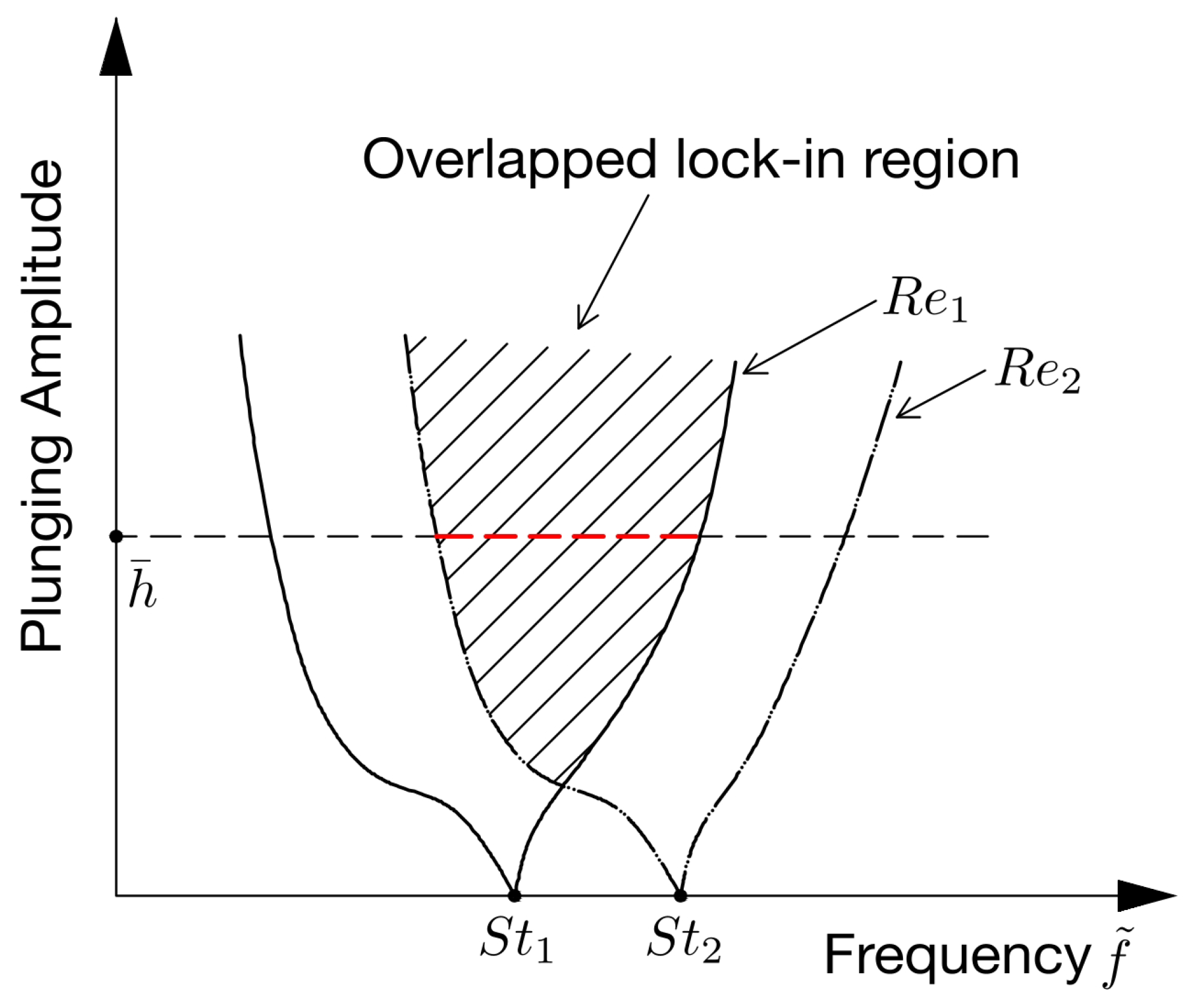
In previous works of Li and Ekici [45,46,47], the One-shot method was modified so that either the amplitude of vibration () or the reduced velocity (similar to here) could be prescribed as the input parameter. However, for the specific problem studied in this work, prescribing and updating is not practical. As illustrated in Figure 4, the lock-in region in terms of frequency and amplitude at a certain Reynolds number features a “V” shape radiating from the point of the natural shedding frequency associated with a stationary cylinder (Strouhal number). Therefore, a finite amplitude oscillation may be in a lock-in region for multiple Reynolds numbers, making the problem ill-posed. As such, the value of is prescribed, and is updated in the One-shot solver for the problem considered in this study.
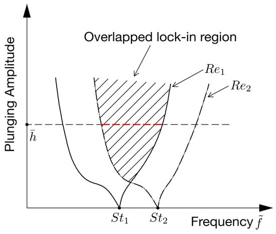
Figure 4.
Overlapped lock-in regions for multiple Reynolds numbers.
3. Results and Discussion
3.1. Validation and Verification of the HB-CFD Solver
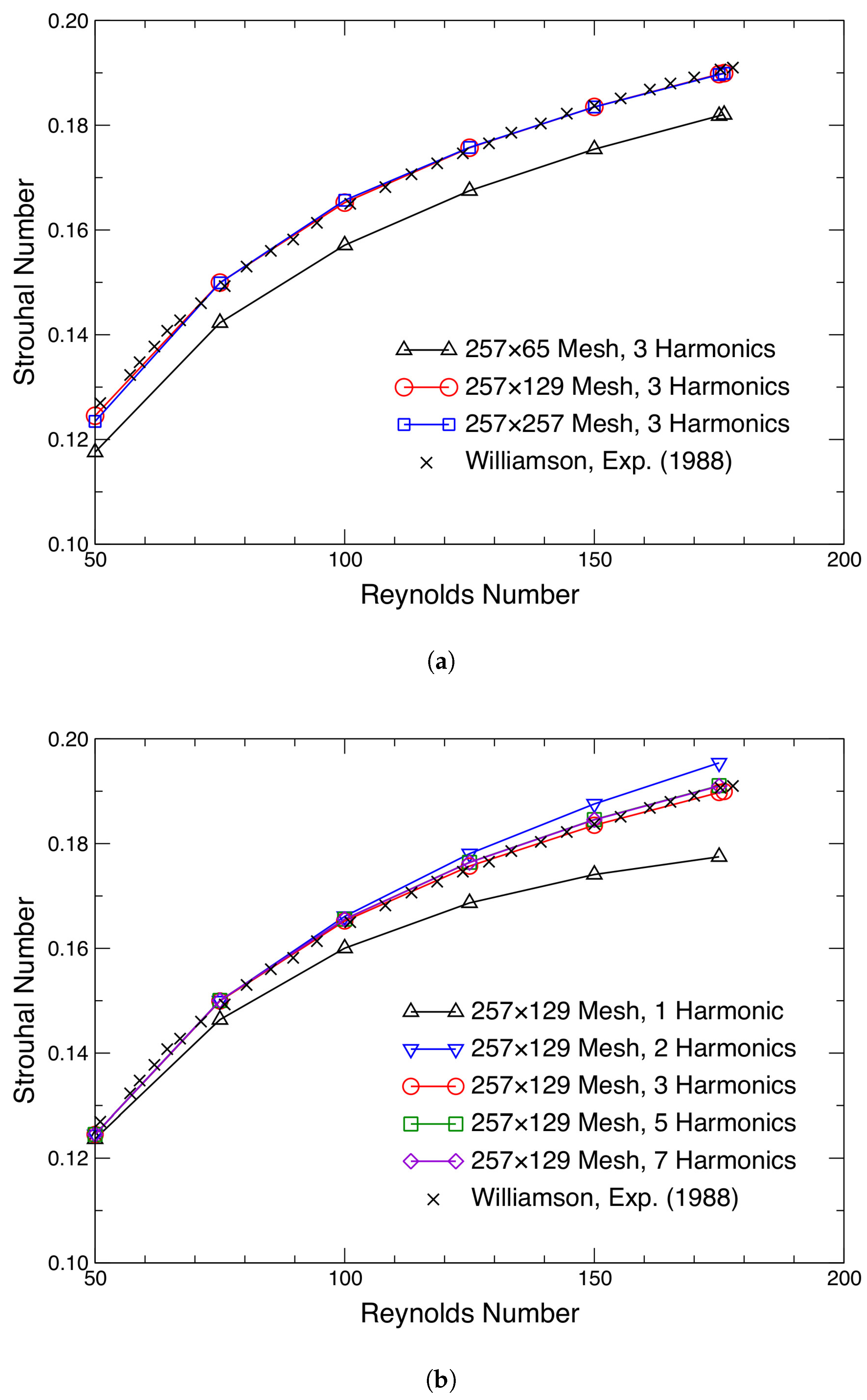
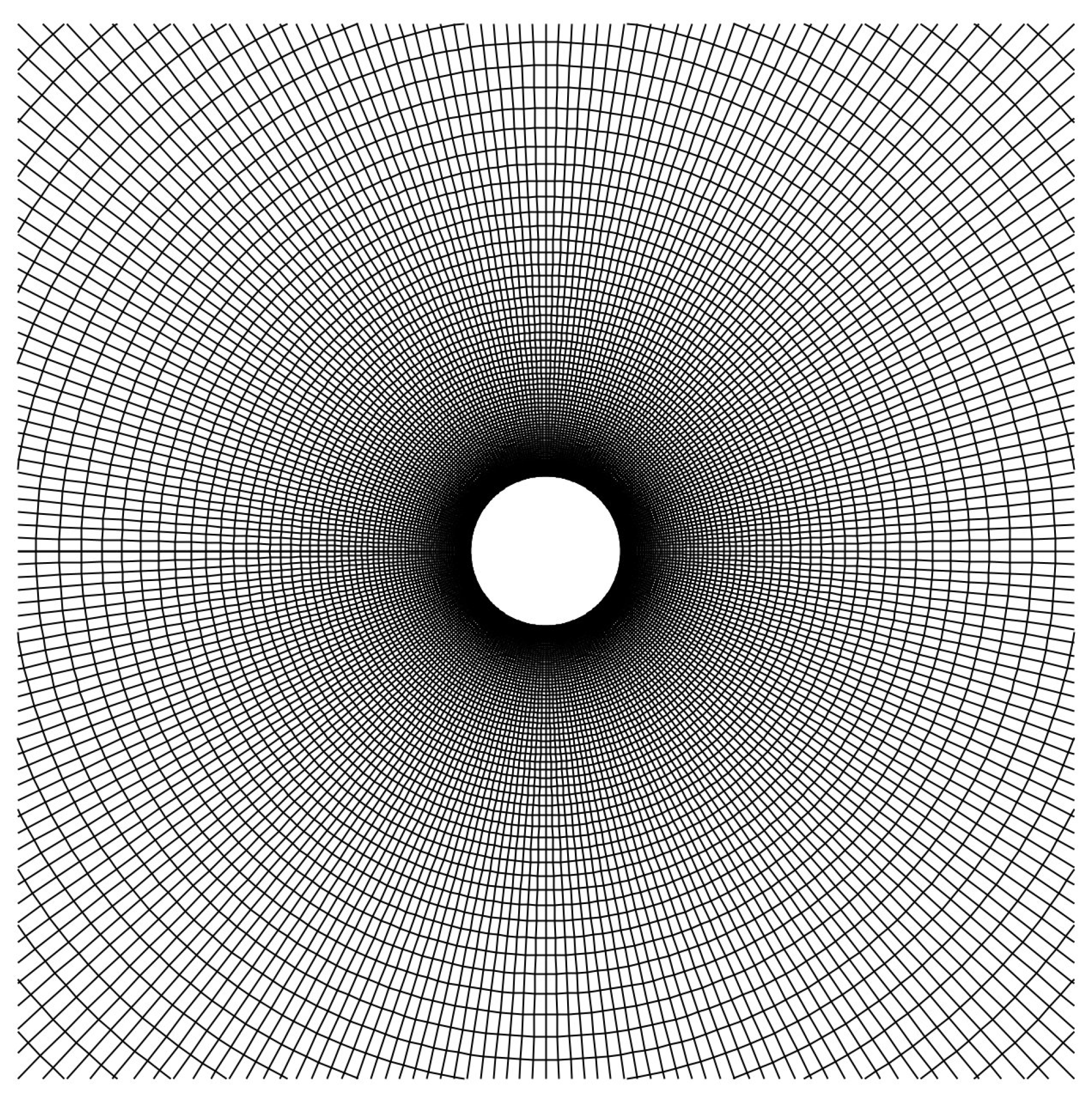
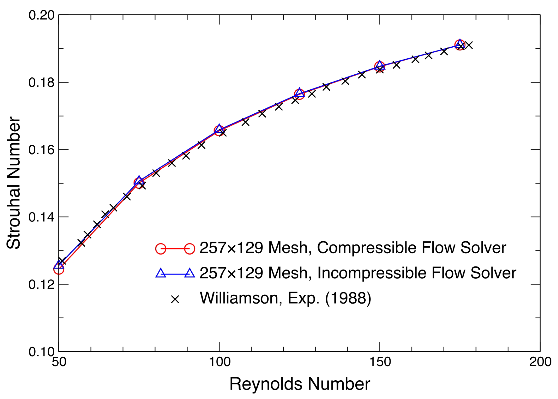
Equation (11) can be solved using the One-shot method provided that the flow field around the cylinder, especially the downstream vortex shedding, is properly resolved. For the case studied in this work, the Reynolds number is kept below 180 so that the vortex shedding remains two-dimensional and laminar. First, a grid convergence study is performed to determine the proper resolution. Three CFD meshes with , and nodes in the circumferential and normal directions are generated, with the far field boundary placed at 20 times the cylinder diameter, and the resolution in the normal direction is doubled successively. The natural vortex shedding frequency for the stationary cylinder (Strouhal number ) is determined by the compressible flow solver using the gradient-based frequency search outlined by Ekici and Huang [24]. In order to trigger the onset of vortex shedding, the cylinder is forced to oscillate rotationally with an amplitude of five degrees in the first 200 iterations. The results are given in Figure 5a together with the experimental data of Williamson [60]. One can see that the mesh with the resolution of appears to be sufficient to capture the Strouhal number (or the vortex shedding frequency), and the results are in excellent agreement with the experimental data. Figure 6 provides a close-up view of this mesh, which will be used for all numerical simulations presented in the following parts of this work. In addition to grid convergence, a “harmonic mode convergence” study is also performed. Figure 5b clearly shows that five harmonics are adequate to reach mode convergence for this case. Although the results of three harmonics are very close to the converged results, five harmonics are used in the following analyses to ensure that the unsteady flow field is properly resolved. The Strouhal number is also predicted by an incompressible solver, and the results are provided in Figure 7. The excellent agreement between compressible and incompressible results justifies the use of the compressible flow solver for this low-Reynolds-number case.
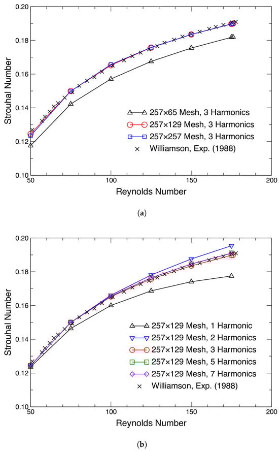
Figure 5.
Grid and harmonic mode convergence study regarding the natural vortex shedding frequency associated with the stationary cylinder (Strouhal number ) at laminar Reynolds numbers: (a) grid convergence; (b) harmonic mode convergence. Adapted from Williamson, Exp. [60].
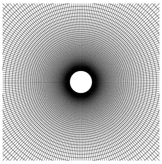
Figure 6.
Close-up view of the 257×129 O-type viscous mesh around a cylinder.
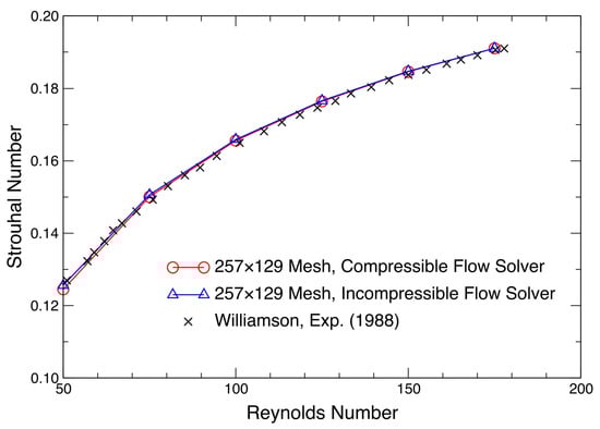
Figure 7.
Comparison of Strouhal number at laminar Reynolds numbers obtained from both compressible and incompressible solvers. Adapted from Williamson, Exp. [60].
In addition to the Strouhal number, the unsteady forces induced by vortex shedding are also determined using both compressible and incompressible flow solvers, which are compared to data reported in the literature in Figure 8. Looking at the magnitude of the lift coefficient, , the current results have a reasonably good agreement with other reported data. Significant differences between the simulation results and the experimental data of Tanida et al. [61] may be partly due to the presence of unsealed gaps in the towing tank of the experiments, which could cause a dramatic reduction in unsteady lift forces [62]. Although minor discrepancies exist between the compressible and incompressible solvers, the overall agreement is very good.
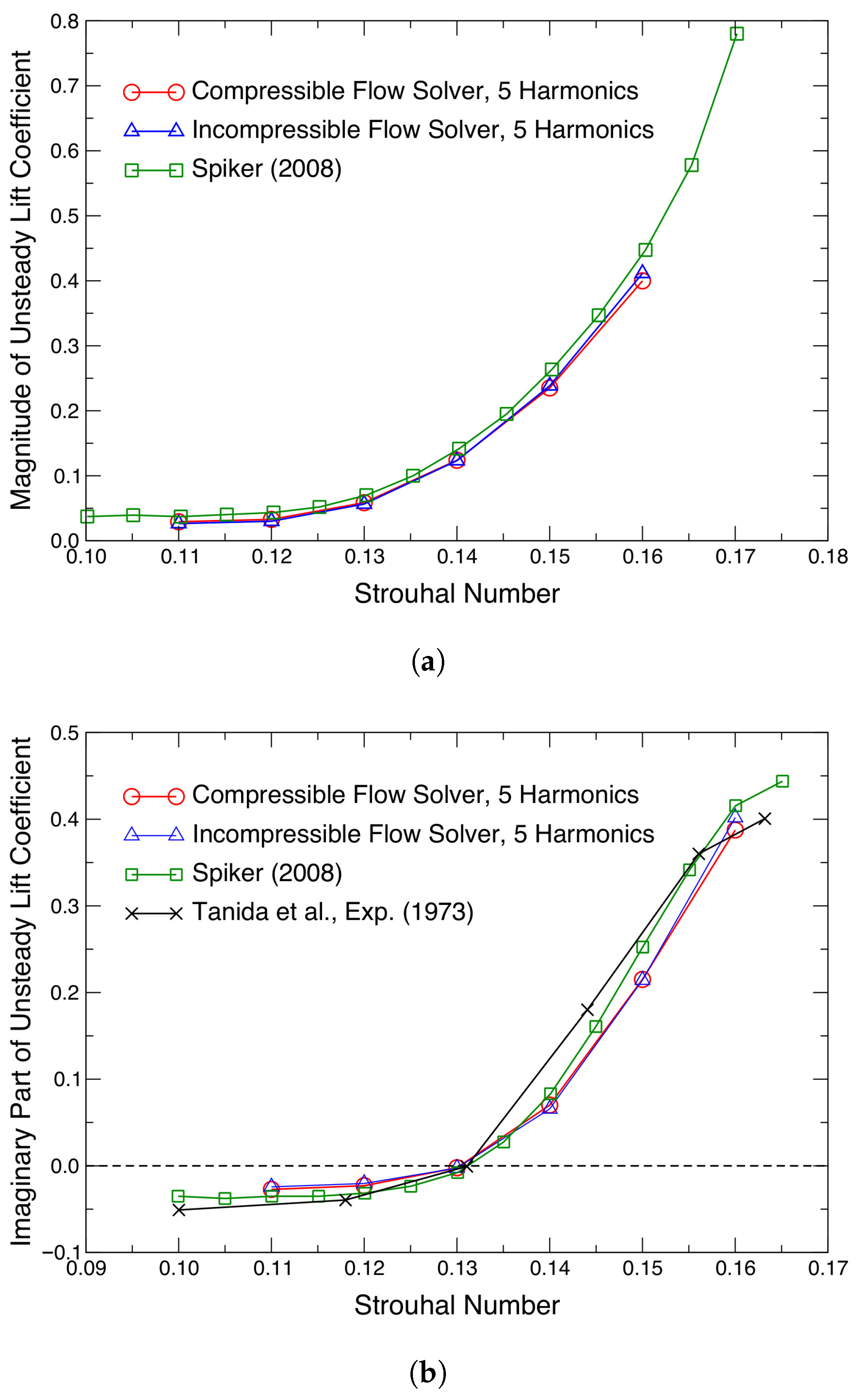
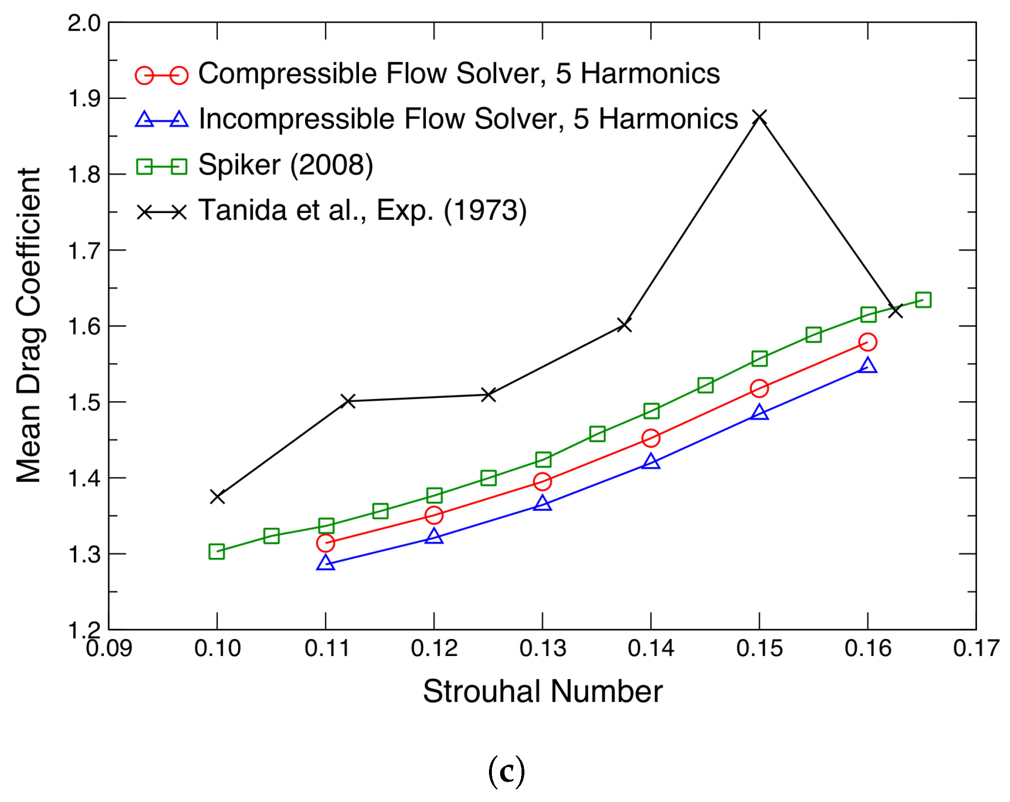
In order to further verify the HB-CFD solver, the cylinder is forced to heave at = 80 with an amplitude of subject to different excitation frequencies in the lock-in range. The resultant unsteady forces are plotted in Figure 9. One can see that the current results for the magnitude and the imaginary part of agree well with other results available in the literature. A positive imaginary part of indicates a fluidelastically unstable case. The results of also have a good agreement with those of Spiker [30], although relatively large discrepancies are observed compared to the experimental results of Tanida et al. [61]. Similar to the results shown in Figure 8, although discrepancies of exist between compressible and incompressible solvers, the results of from two solvers have a very good agreement. Considering that only the lift force contributes to the fluid dynamic forcing for a 1-DOF VIV setup (such as the one considered here), the compressible HB flow solver is used for the results presented hereafter. Readers are referred to the earlier works of Huang and Ekici [54] and Djeddi and Ekici [63] for more verification studies of the in-house HB-CFD solver on various vortex shedding cases of oscillating cylinders.
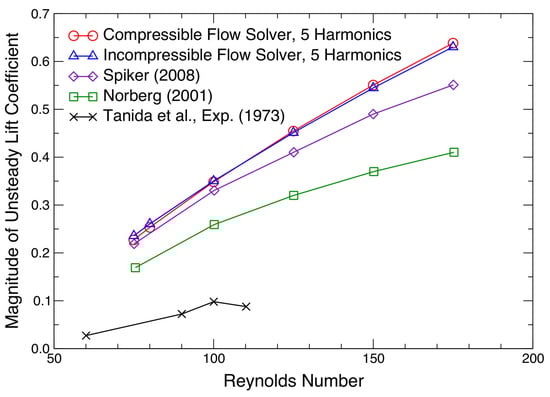
Figure 8.
Unsteady lift coefficient for a stationary cylinder due to natural vortex shedding at low Reynolds numbers. Adapted from Spiker [30], Norberg [64], Tanida et al. [61].
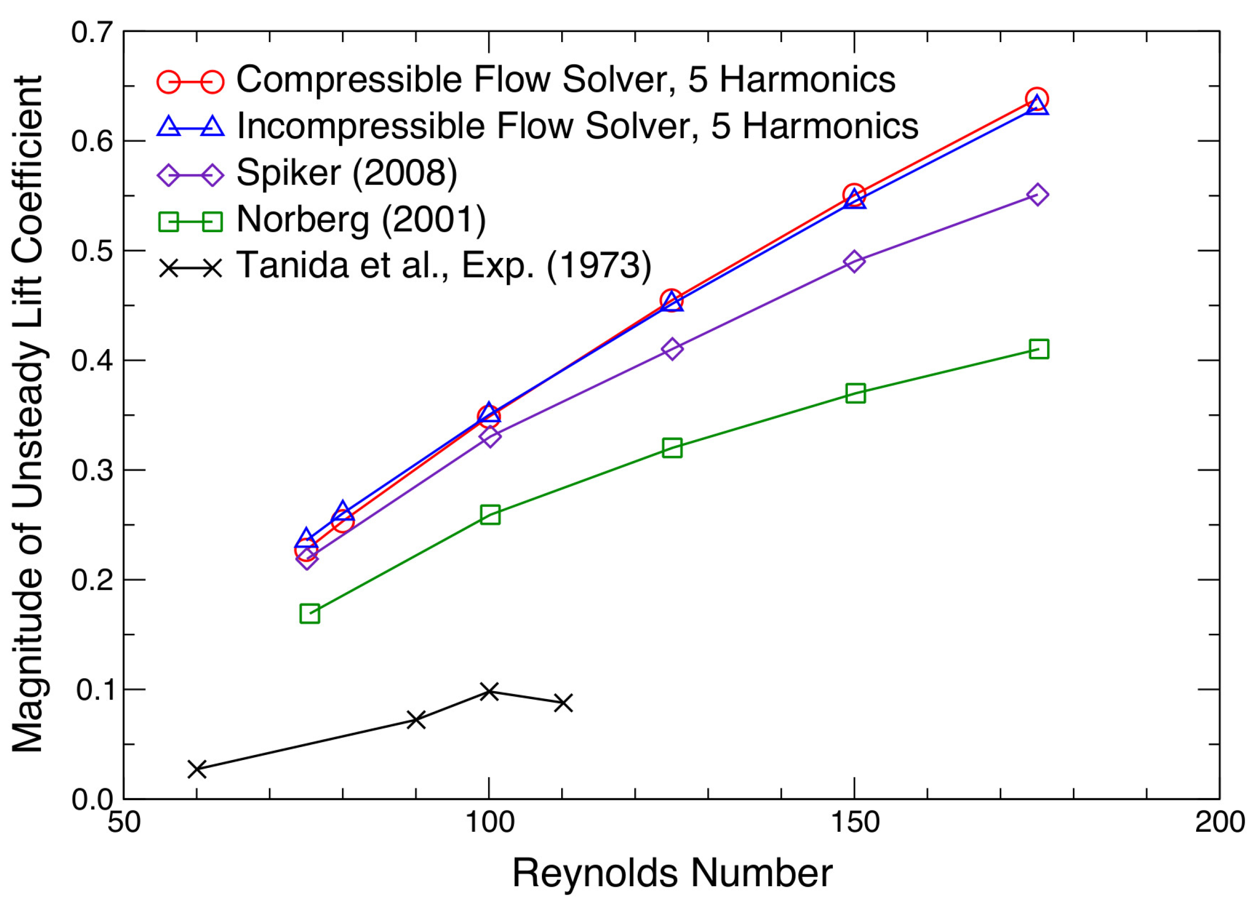
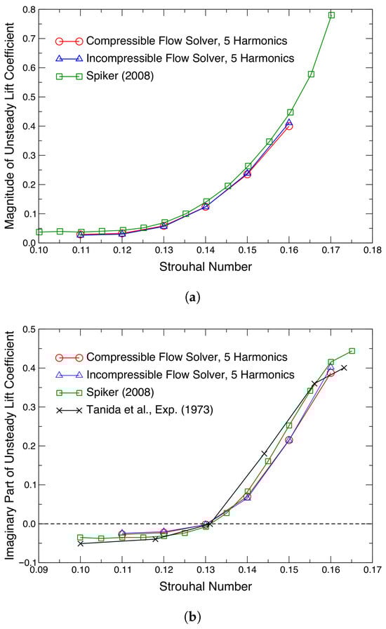
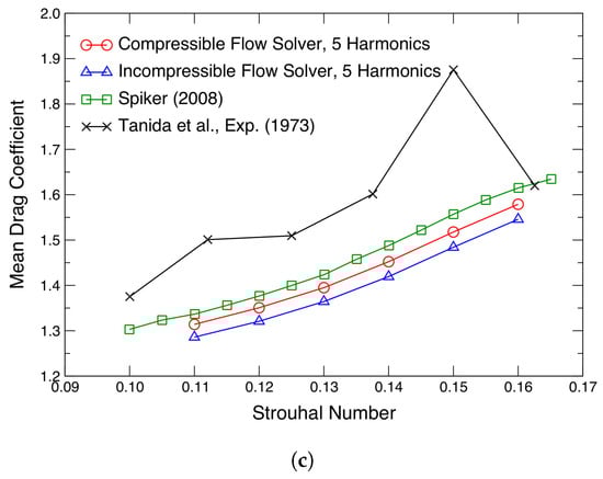
Figure 9.
Unsteady forces of cylinder undergoing plunging of amplitude , = 80: (a) magnitude of unsteady lift coefficient, ; (b) imaginary part of unsteady lift coefficient; (c) mean drag coefficient, . Adapted from Spiker [30], Tanida et al. [61].
3.2. The VIV Results
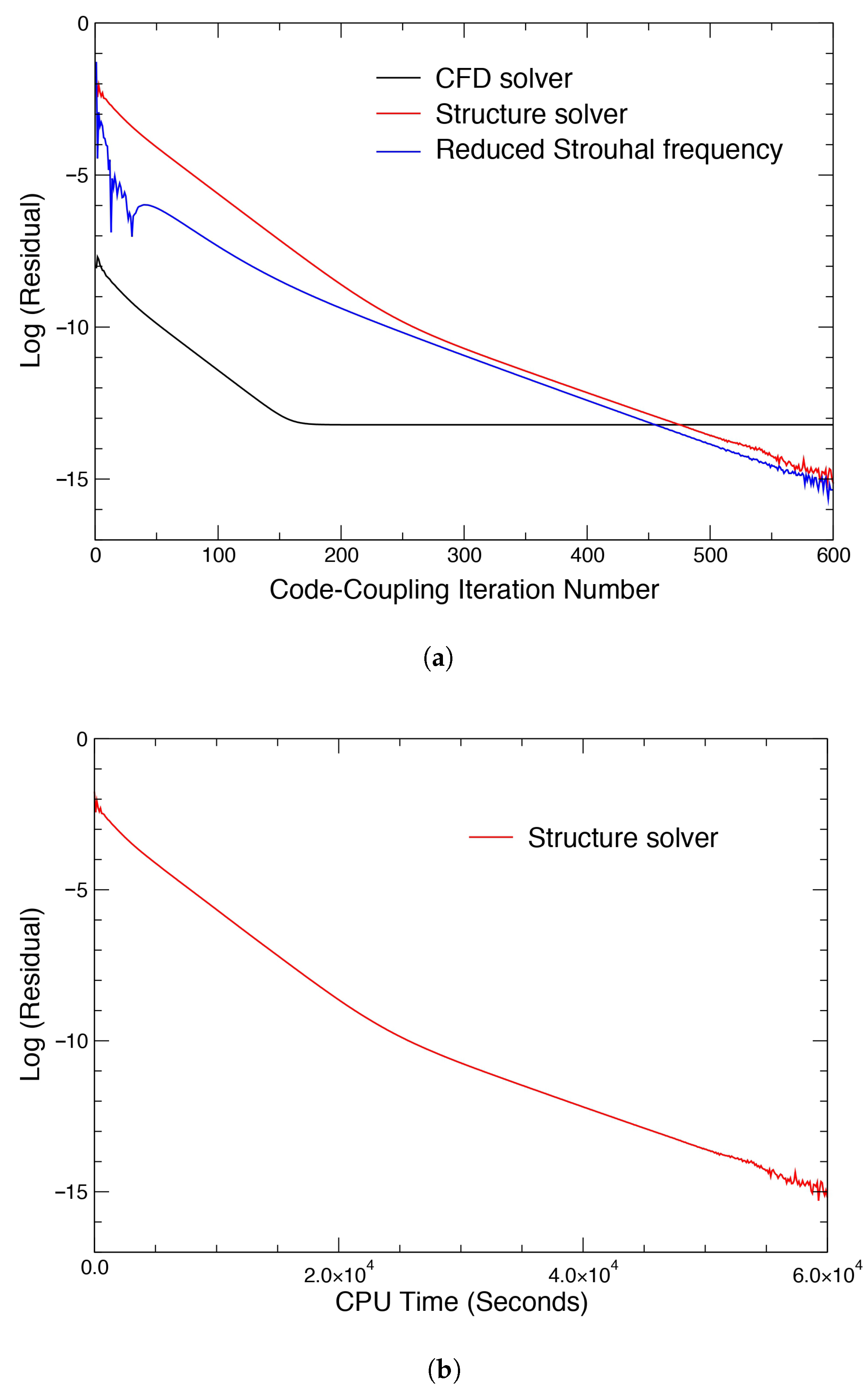
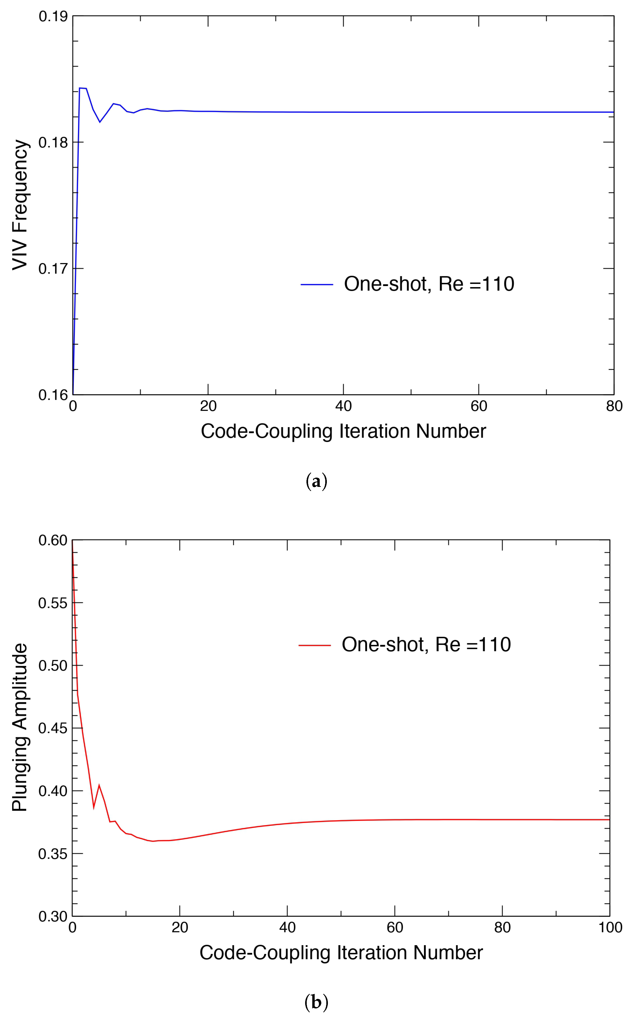
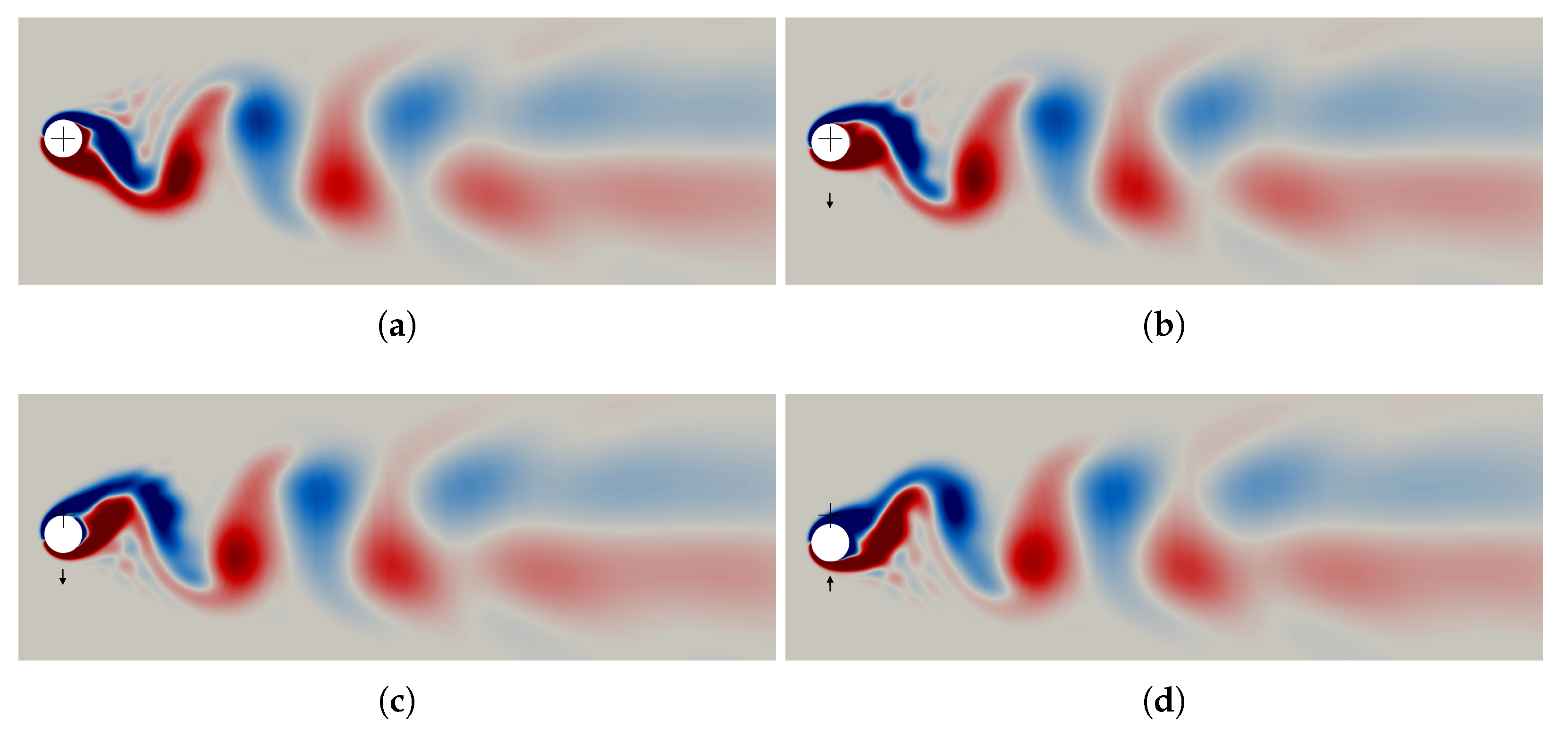
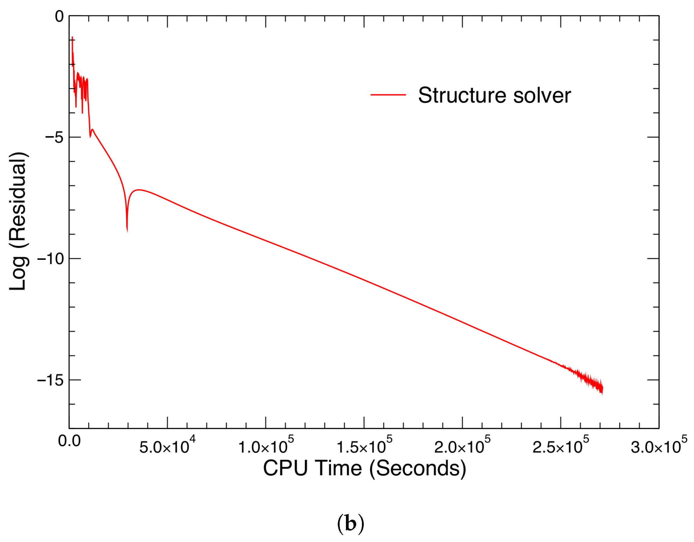
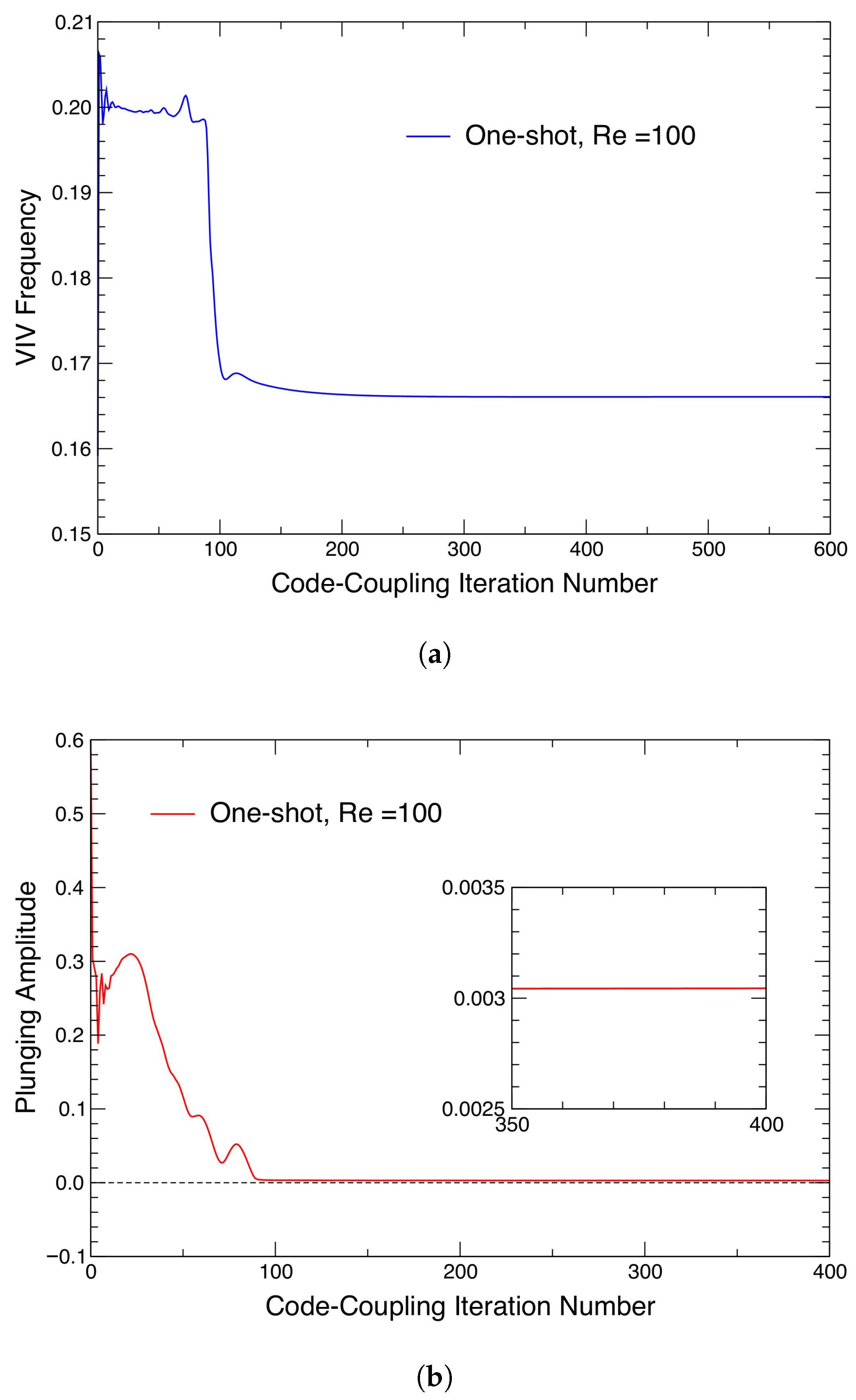
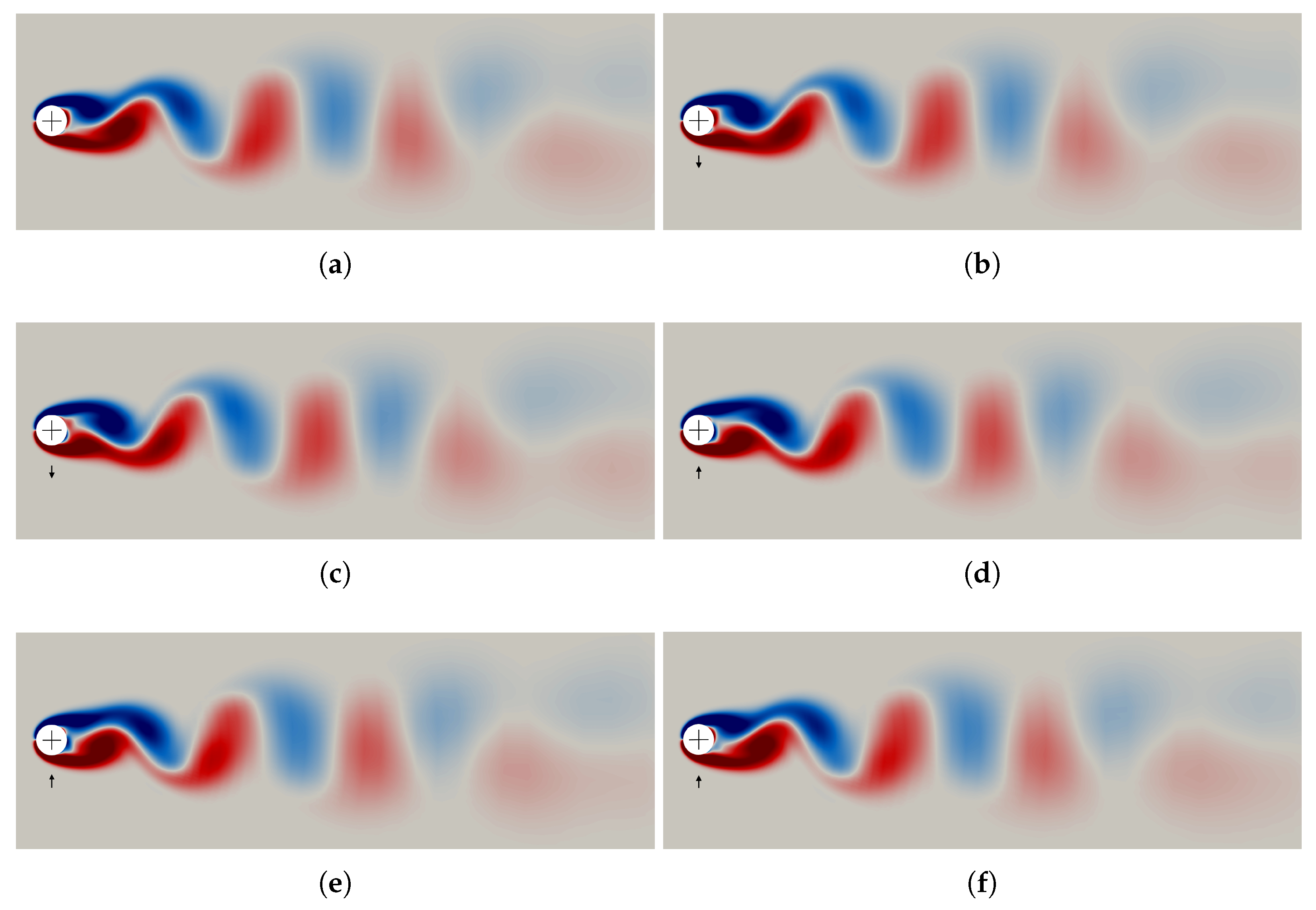
In this section, the One-shot method is applied to model the one-DOF VIV system of Anagnostopoulos and Bearman [6]. Compilations of available results of this case can be found in the works of Williamson and Govardhan [1], Kaneko et al. [17], and He et al. [65,66,67]. It has been extensively reported in the literature that both lock-in and non-lock-in types of vibrations exist for low-Reynolds-number laminar flow regimes. At the present time, since the One-shot solver is able to deal with only one fundamental frequency, the lock-in type of vibration is studied here. To begin with, the limit cycle response at = 110 is investigated. The parameters for the One-shot solver are provided in Table 1. In practice, we have found the One-shot solver to be robust across a wide range of parameter values. In this case, the implicit CSD solver is set to run at every 100 iterations of the CFD solver, and the pseudo-time step for the CSD solver is taken to be . Although not shown here, this combination of solver setup yields an optimal convergence rate. The convergence history as well as the CPU time required for this case are plotted in Figure 10. It is seen that all limit cycle solutions are driven to convergence simultaneously within 600 One-shot iterations. In addition, Figure 11 shows that the change in values of VIV frequency, , and plunging amplitude, , become indiscernible within only dozens of iterations. The vortex shedding associated with plunging vibration is presented by instantaneous vorticity contours at every other sub-time level in Figure 12. One can see that vortices shed in a “2S mode” (two single vortices per period) initially, and then transition to the “C(2S) mode”, where vortices coalesce in the wake [68,69]. This wake pattern is similar to that reported by Bahmani and Akbari [13,70].

Table 1.
One-shot solver parameters for the case of = 110.
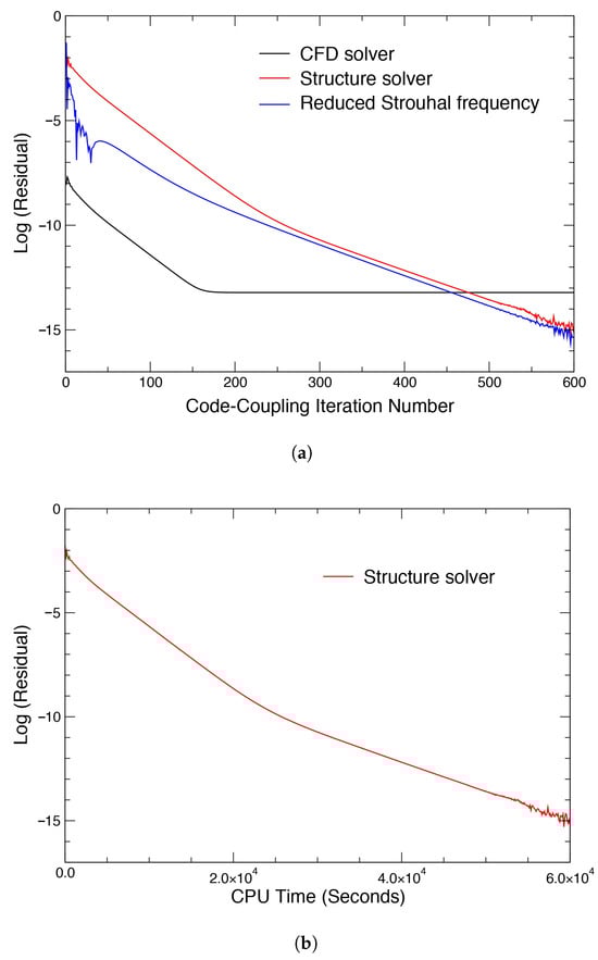
Figure 10.
Convergence history of residuals of VIV case = 110: (a) residuals against One-shot code-coupling iteration number; (b) residual against computational cost.
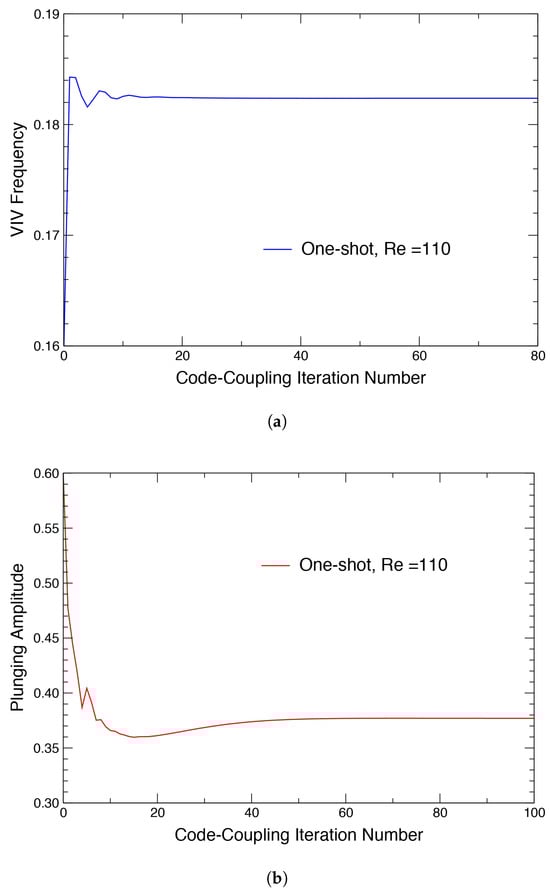
Figure 11.
Convergence history of VIV frequency and plunging amplitude of the VIV case = 110. (a) VIV frequency, ; (b) Plunging amplitude, .
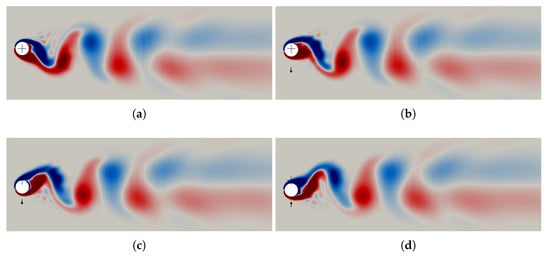
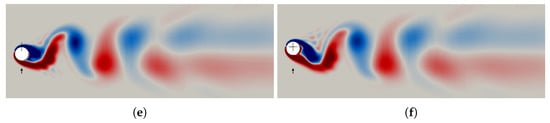
Figure 12.
Unsteady vorticity contours showing vortex shedding with plunging cylinder at = 110. The arrows indicate the motion direction and the crosses mark the cylinder center at the first sub-time level. (a) Sub-time level 1; (b) sub-time level 3; (c) sub-time level 5; (d) sub-time level 7; (e) sub-time level 9; (f) sub-time level 11.
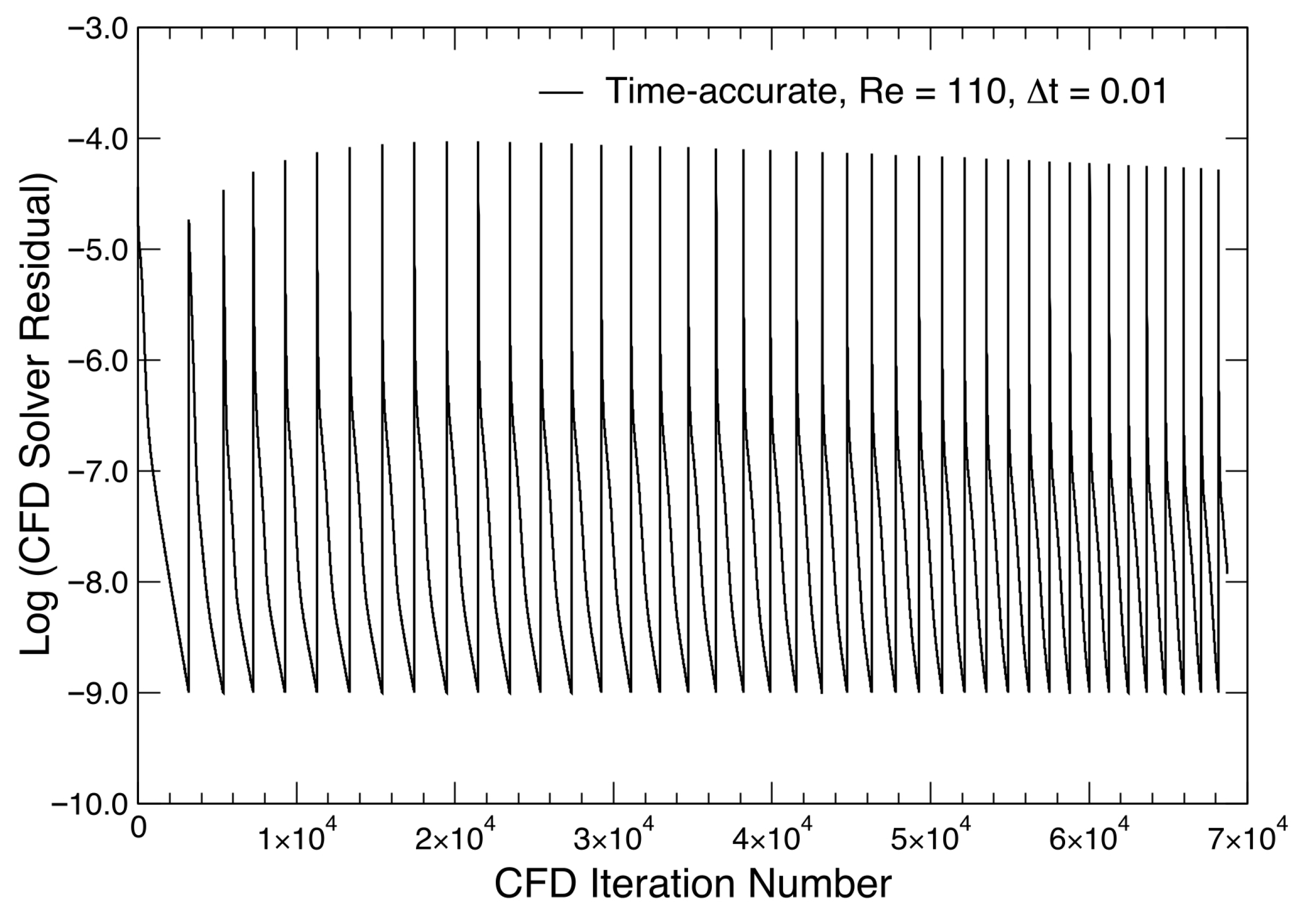
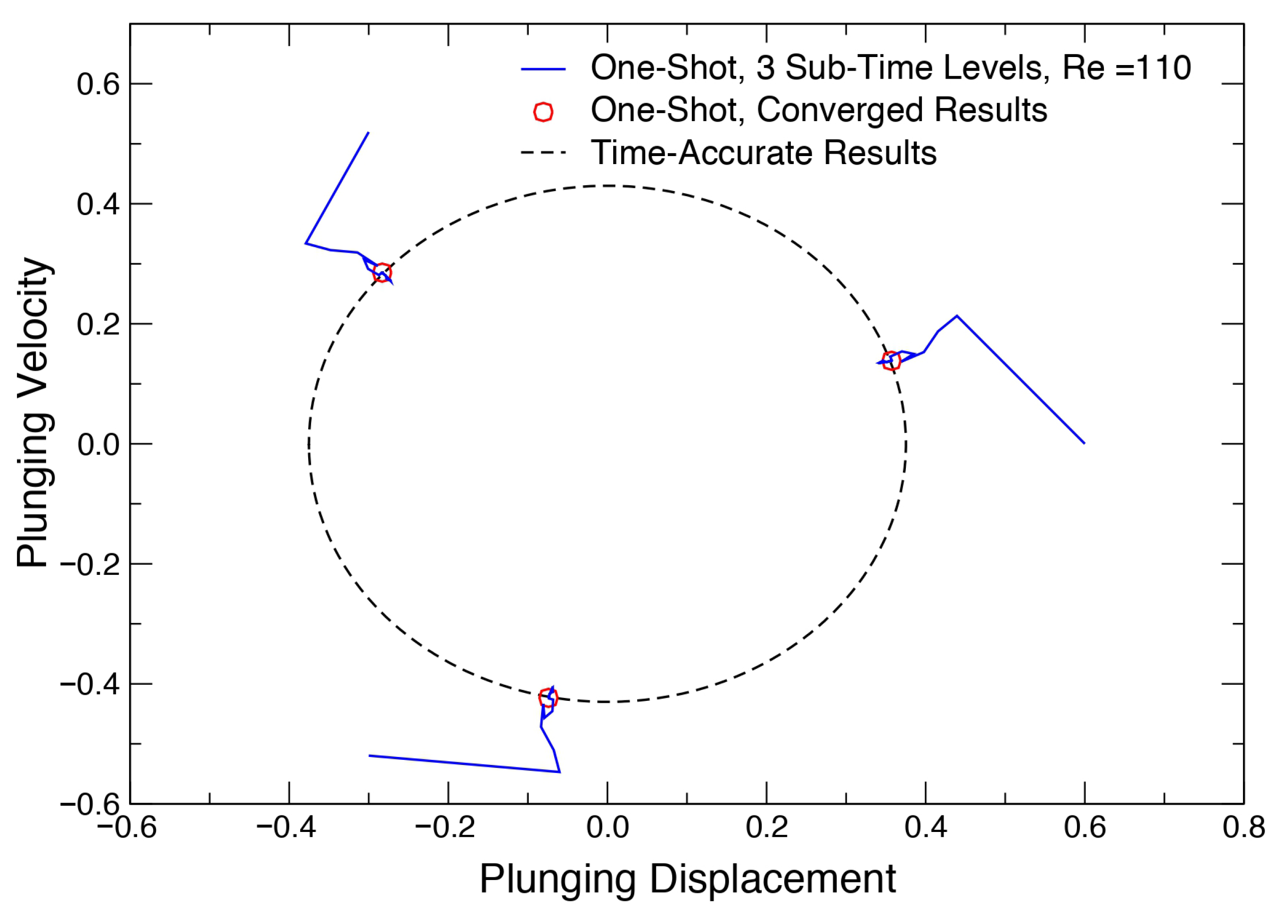
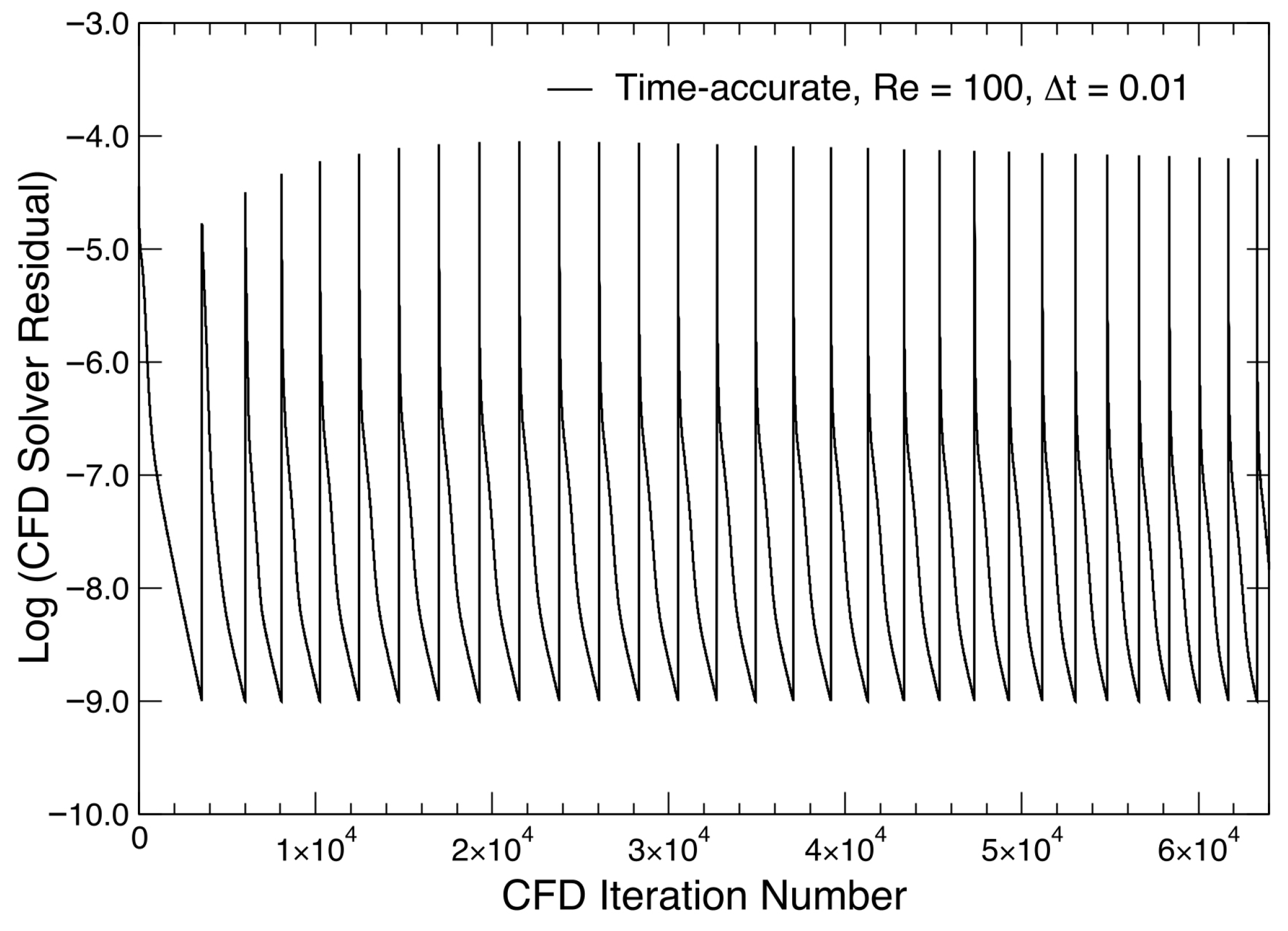
For verification purposes, the same case is also simulated using our in-house time-accurate solver based on the loosely-coupled, second-order time-accurate generalized serial staggered (GSS) algorithm originally proposed by Geuzaine et al. [71]. Readers are referred to an earlier work of Li [58] for details about this approach and the solver. For this case, the residual of the CFD solver is driven down at least four orders at every physical time step, as shown in Figure 13. The time history of plunging displacement and lift coefficient are plotted in Figure 14. It can be seen that although the initial transient before reaching the stable periodic pattern is reduced by starting with an amplitude that is close to the final solution, the cost of the time-accurate solver is still over ten times higher than that of the One-shot solver, as evidenced in Figure 10b and tabulated in Table 2. This demonstrates the biggest advantage of the One-shot method. Moreover, results of and from both solvers (time-accurate and One-shot) are also reported in Table 2, showing excellent agreement and instilling confidence in the One-shot method. Figure 15 shows the convergence history of the three sub-time levels of the cylinder motion in the phase plane, in which the converged points lie on top of the orbit from the time-accurate results.
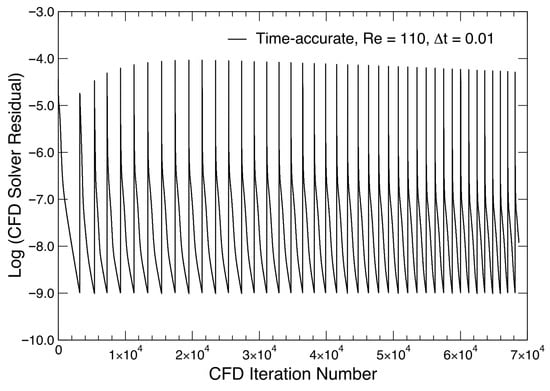
Figure 13.
Inner iteration residuals for early physical time steps of the time-accurate run, = 110.
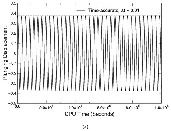
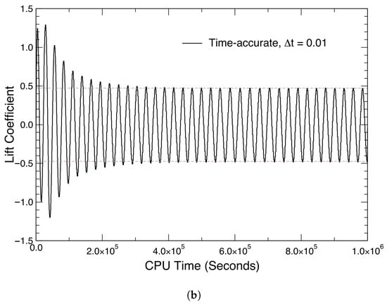
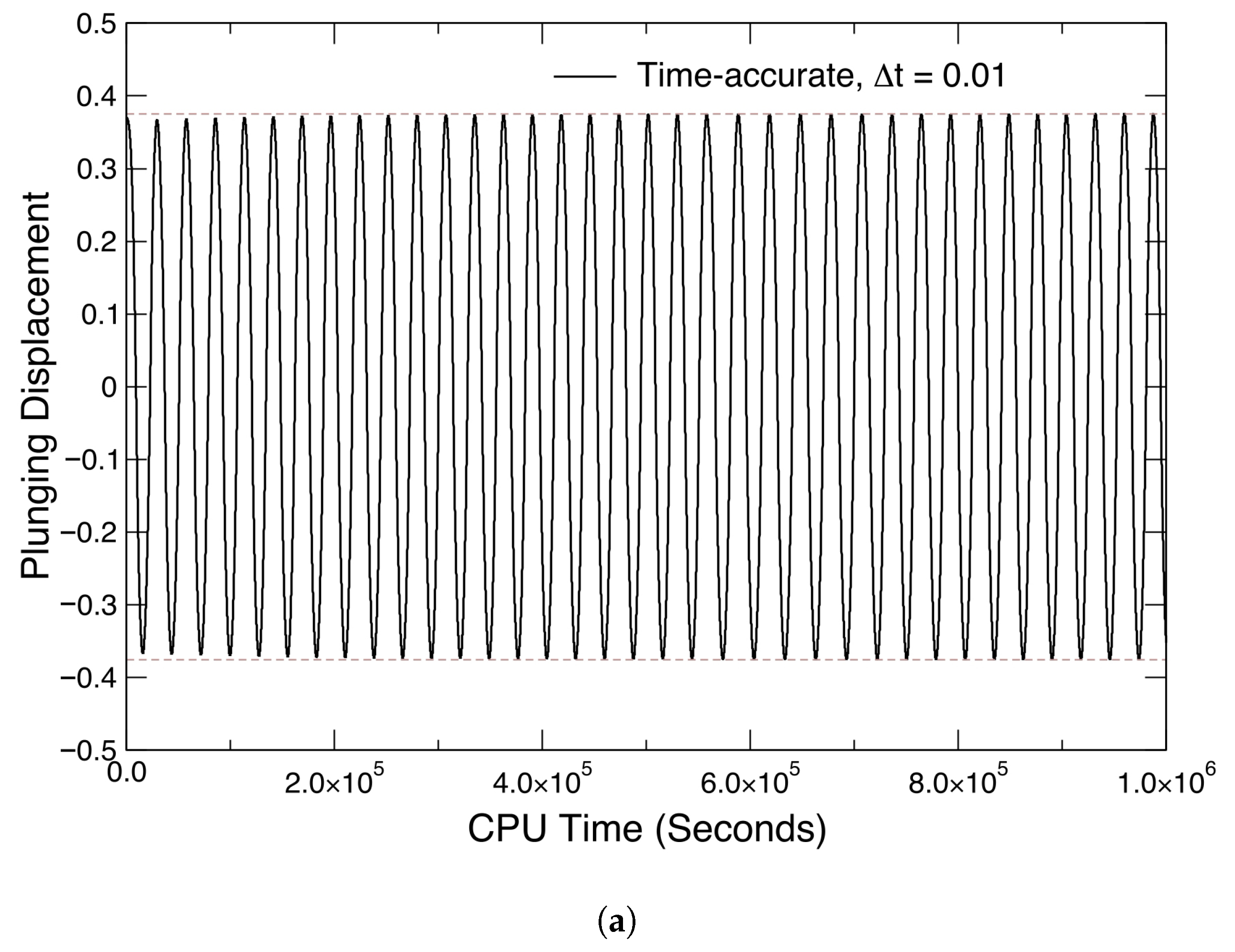
Figure 14.
Time-accurate results of VIV case = 110. The converged amplitudes are indicated by dashed lines. (a) Plunging displacement, ; (b) lift coefficient, .
Table 2.
Comparison of One-shot and time-accurate method for VIV prediction at = 110.
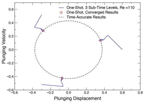
Figure 15.
Convergence of the three sub-time levels for the cylinder motion in the One-shot solver, = 110.
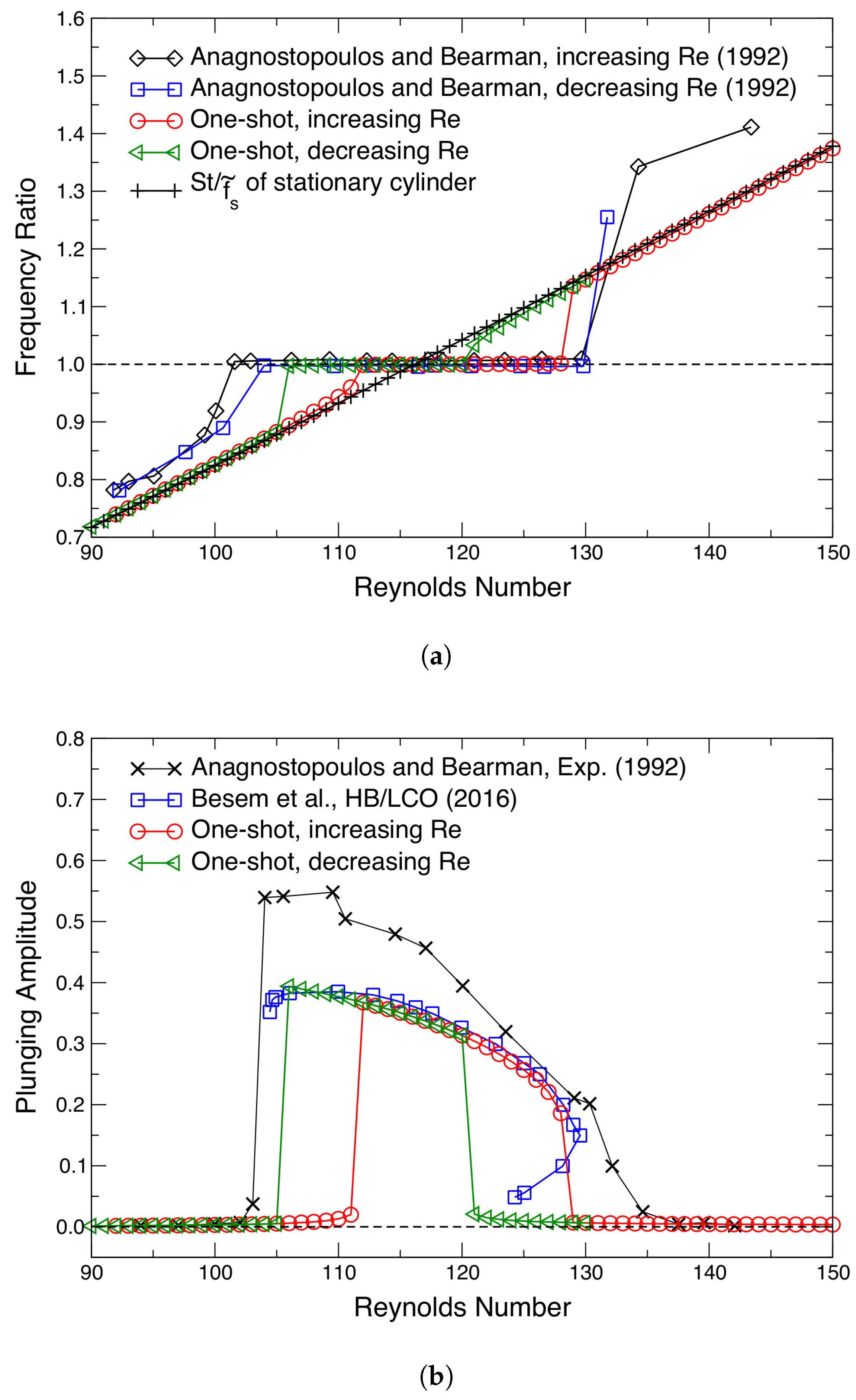
Next, to identify the lock-in region for this configuration, the Reynolds number is varied by first increasing and then decreasing its value in the forward and backward directions, respectively. A step size of = 1 is used in this process, in which the previous converged solution is used as the initial condition for the run of the next value. Fully converged results are obtained over the entire range of tested , of which the ratio of to the structural natural frequency, , and the VIV amplitude are given in Figure 16. The data points from the experiment of Anagnostopoulos and Bearman [6] are also plotted, as well as some other available data from the literature. One can see that the resonant range of is roughly from 104 to 130, as indicated in Figure 16a, where the plunging amplitudes are dramatically larger than those outside of this range, as shown in Figure 16b.
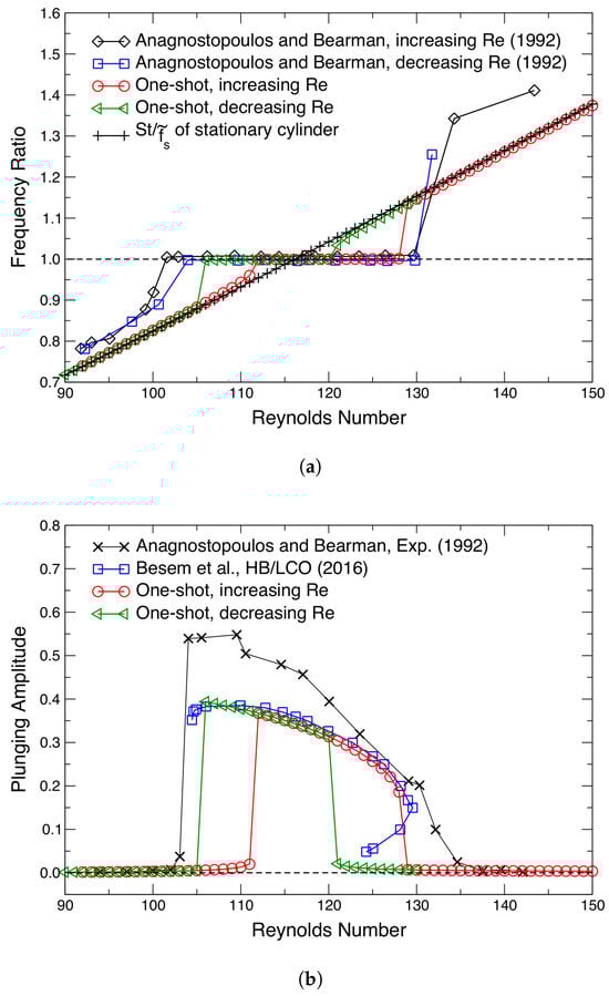
Figure 16.
Frequency ratio and plunging amplitude of the one-DOF cylinder VIV system for Reynolds numbers in the laminar, two-dimensional flow regime: (a) frequency ratio of VIV cases, , and of stationary cylinder, ; (b) plunging amplitude, . Adapted from Anagnostopoulos and Bearman [6], Besem et al. [33].
As can be seen, the results indicate a hysteresis between the sweeps in two opposite directions. The frequency ratio calculated for the Strouhal number (the natural vortex shedding frequency associated with a stationary cylinder, as presented in Figure 5) is also provided. When is increased, the VIV system oscillates at the Strouhal frequency at relatively low before reaching the value around 110, when the frequency starts to deviate and locks to the structural natural frequency at . Meanwhile, the resonance effect increases the amplitude dramatically. After this initial jump, the amplitude continues to reduce until = 128, where the returns back to the Strouhal frequency. The amplitude also drops down to a very small value due to the absence of the resonance effect. Similar jumps are observed when the value of is decreased, resulting in a hysteresis. The combined sweeps show a traditionally recognized lock-in (resonance) range of from 106 to 128. Although the amplitudes are under-predicted compared to the experimental data, the profile has a relatively good agreement with the results of Besem et al. [33] that were obtained using an HB/LCO solver. Similar observations can be made from another compilation of numerical and experimental data reported by He [72]. Note that no hysteresis was reported by Anagnostopoulos and Bearman [6]. Inspired by the explosive type of LCO depicted in Li and Ekici [45], the hysteresis found in this case indicates that unstable LCO branches may exist. This is a possible explanation for the second set of lower amplitude solutions of Besem et al. [33] at from around 125 to 130. This is in some ways similar to the unstable branch in the explosive type of LCO. Unfortunately, unstable branches are not captured for the problem studied here. This is due to the fact that amplitude cannot be prescribed in the current implementation of the One-shot method, as explained in Section 2.2.2.
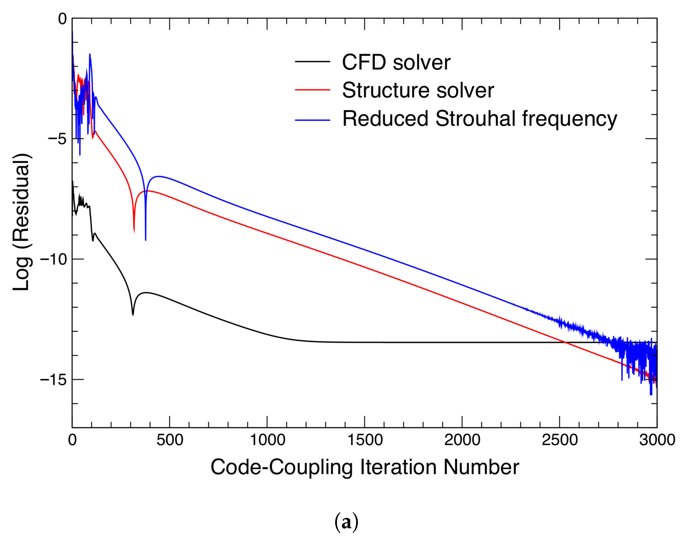
As mentioned earlier, previous works in the literature reported that the vibrations outside of the resonance range were non-lock-in. However, the One-shot solver predicts lock-in oscillations outside of the resonance range with small vibration amplitudes. For demonstration purposes, the VIV condition at = 100, which is below the resonance range, is considered next. In order to assess the robustness of this code-coupling approach, this case is rerun using the same setup and initial conditions as in the previous case of = 110 (see Table 1), in which the initial (0.6) is orders of magnitude larger than the final result. As expected, the residuals of both fluid and structural solvers as well as the frequency converge simultaneously; these are plotted in Figure 17. Compared to the previous case of = 110, the One-shot solver takes about four times more computational cost to reach full convergence. Despite this, the One-shot solver is still around 15–20 times faster than the time-accurate approach. The values of and reach convergence visually within a few hundred iterations, as shown in Figure 18. In addition, the instantaneous vorticity contours at every other sub-time level are presented in Figure 19, which shows a “2S mode” vortex shedding. For this case, the motion of the cylinder is barely visible due to the small vibration amplitude.

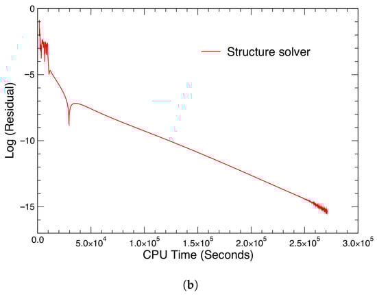
Figure 17.
Convergence history of residuals of VIV case = 100: (a) residuals against One-shot code-coupling iteration number; (b) residual against computational cost.
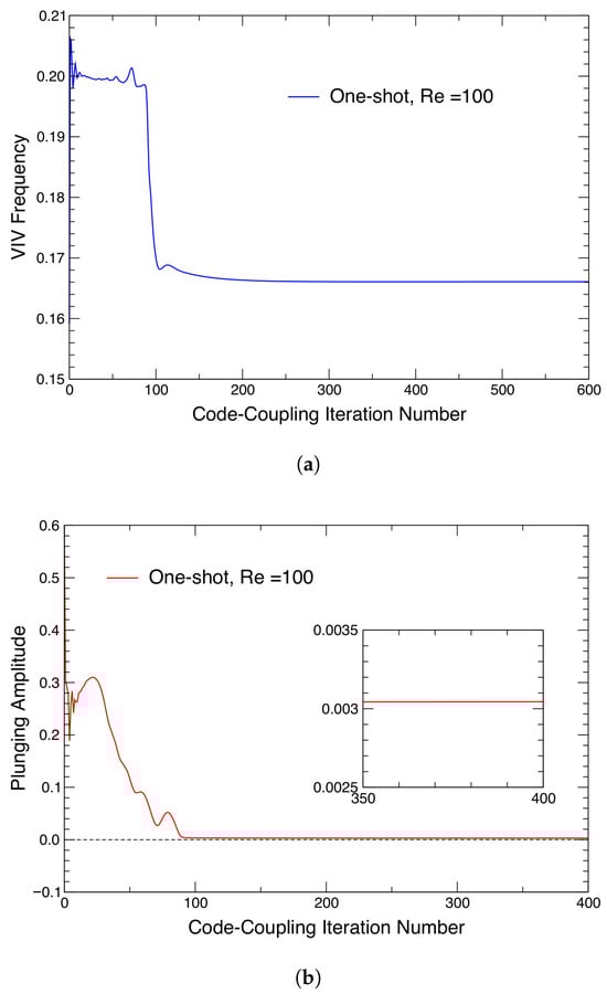
Figure 18.
Convergence history of VIV frequency and plunging amplitude of the VIV case = 100: (a) VIV frequency, ; (b) plunging amplitude, .

Figure 19.
Unsteady vorticity contours showing vortex shedding with plunging cylinder at = 100. The arrows indicate the motion direction, and the crosses mark the cylinder center at the first sub-time level. (a) Sub-time level 1; (b) sub-time level 3; (c) sub-time level 5; (d) sub-time level 7; (e) sub-time level 9; (f) sub-time level 11.
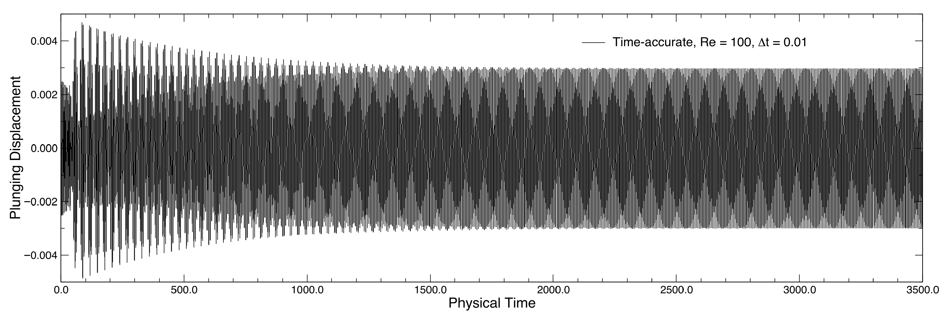
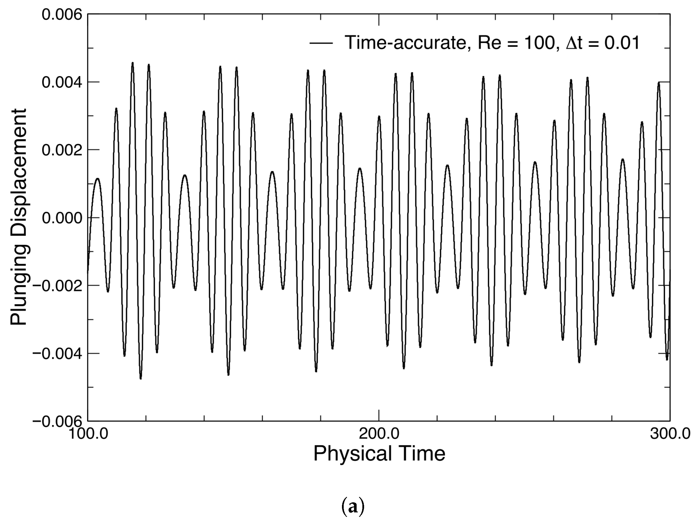
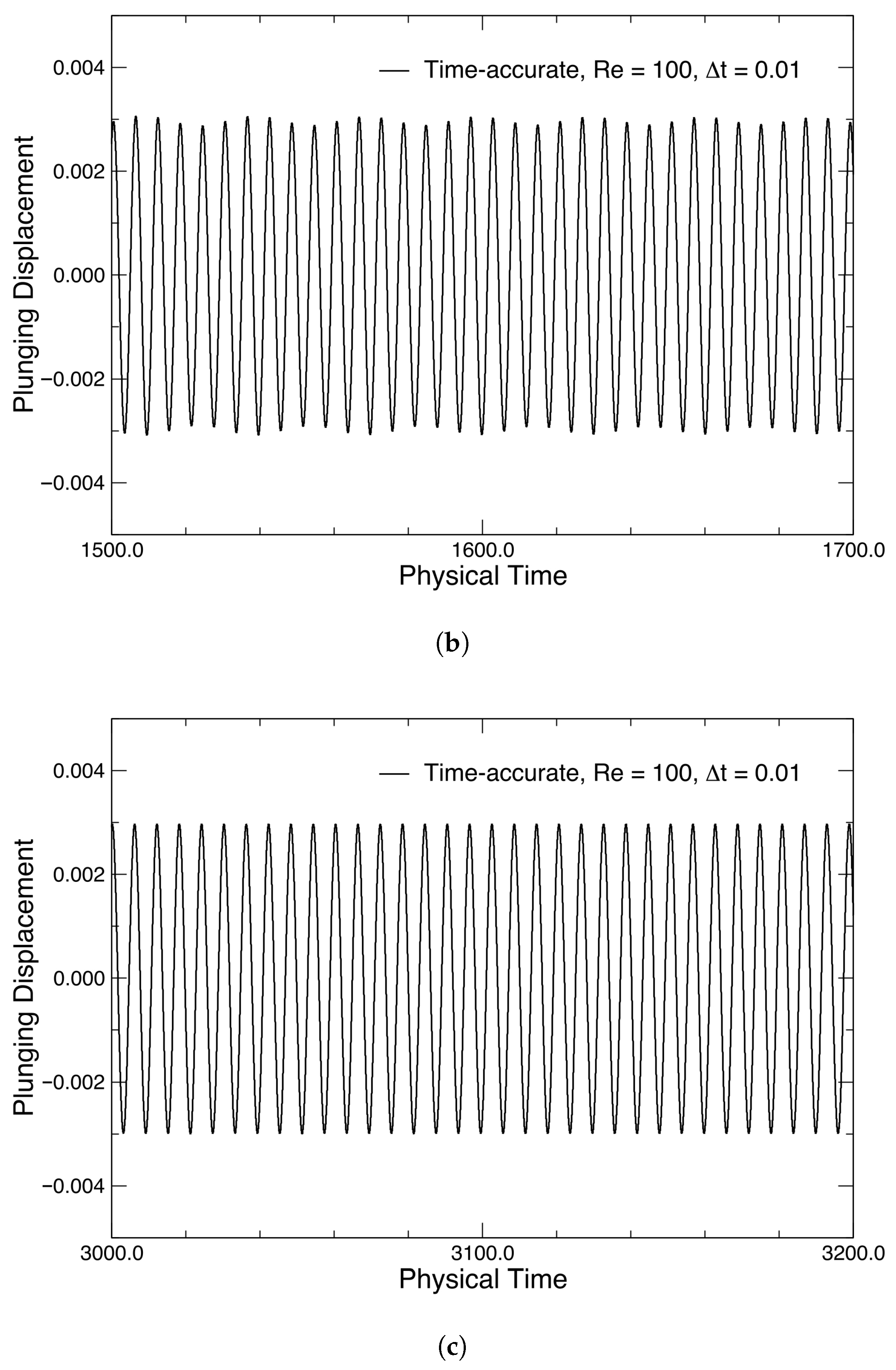
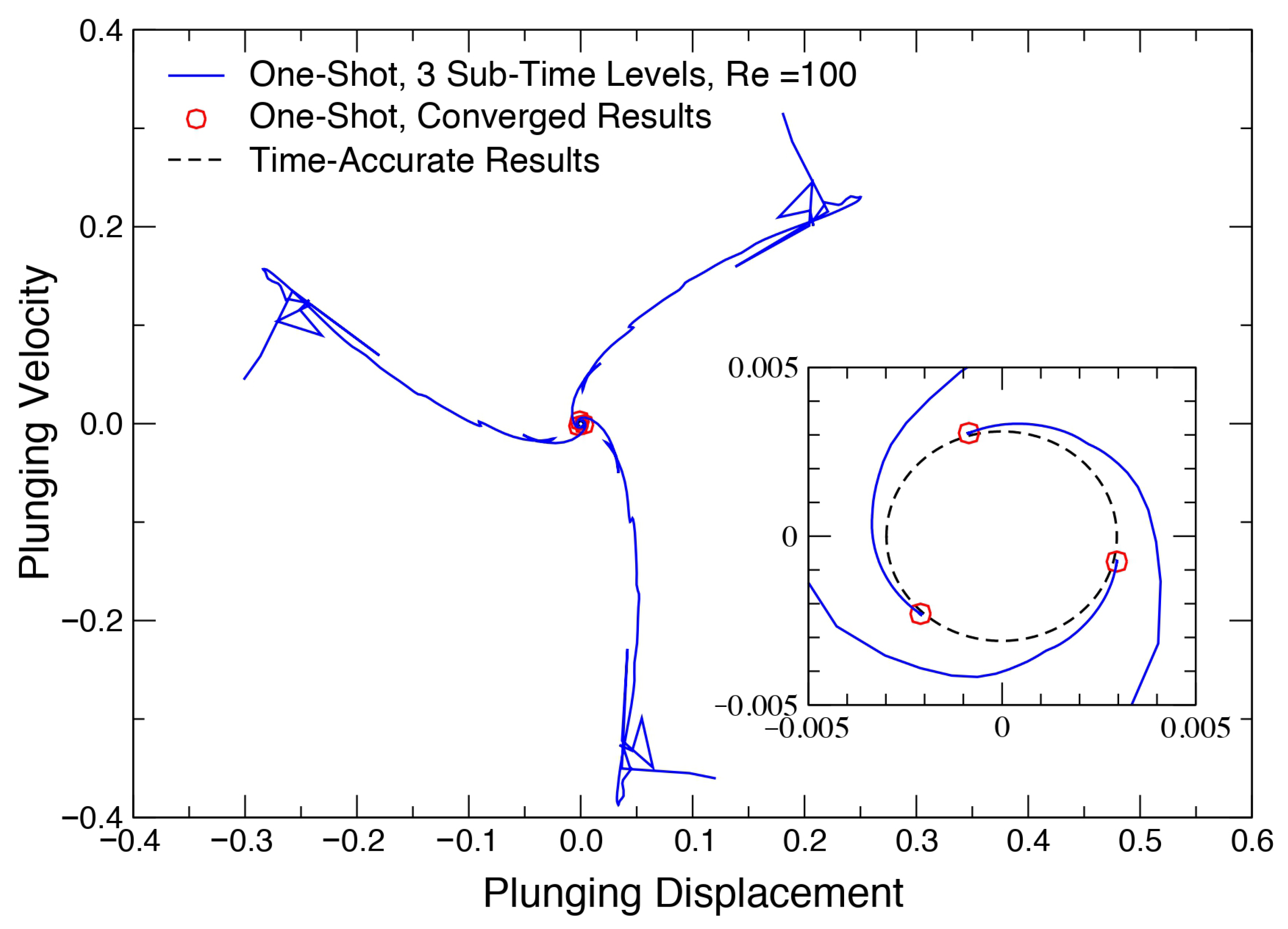
In order to confirm this observation, the in-house time-accurate solver is run for = 100 for an extended period of time. The residual of the CFD solver for a couple of time steps is shown in Figure 20. The evolution of plunging motion is plotted in Figure 21, from which one can see that the vibration at this Reynolds number is initially non-lock-in, which means at least two different frequencies dominate the system, which leads to the observed beat or modulation. However, the strength of the beat weakens gradually over time until the vibration becomes purely lock-in. Details of this change are shown in Figure 22 at three different time intervals. Note that a few other studies reported a similar behavior [65,66,73,74]. However, some of the time-accurate solutions in those works were possibly terminated before the fully lock-in case was recovered, not indicating a transition process as presented in this work. The time-accurate results of and at the final lock-in status are tabulated in Table 3, which match the One-shot results fairly well. This agreement can also be observed from the phase plane plot in Figure 23, in which the three sub-time levels of the cylinder motion in the One-shot solver converge to different points on the trajectory of the time-accurate results. Once again, due to the inherent assumption of a single fundamental frequency, the One-shot solver only considers the lock-in status without having to go through a transient response.
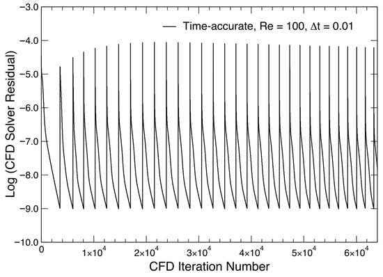
Figure 20.
Residual of CFD solver for a couple of time steps at the beginning of the time-accurate coupled solver run, = 100.
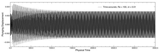
Figure 21.
Time loci of plunging displacement of VIV case = 100.
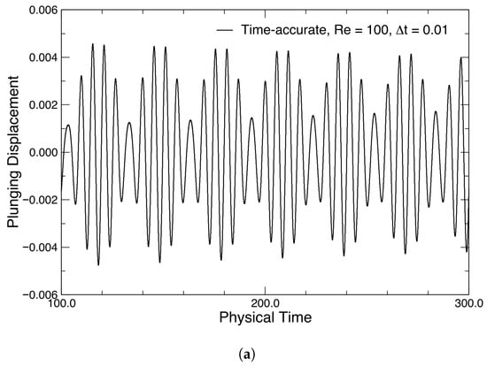
Figure 22.
Time-accurate results at different time slots showing the evolution of vibration from non-lock-in to lock-in, = 100: (a) time from 100 to 300; (b) time from 1500 to 1700; (c) time from 3000 to 3200.
Table 3.
Comparison of One-shot and time-accurate VIV results of = 100.
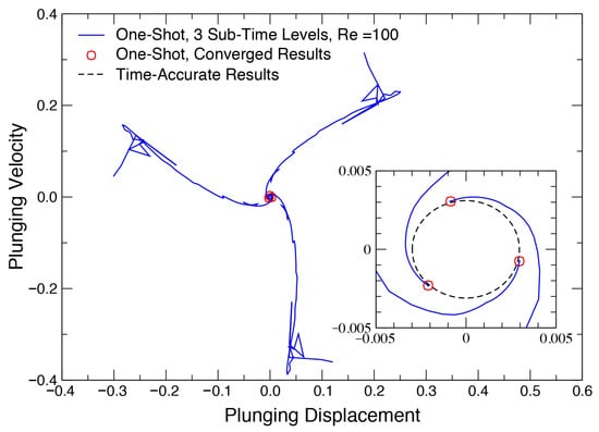
Figure 23.
Convergence of the three sub-time levels for the cylinder motion in the One-shot solver, = 100.
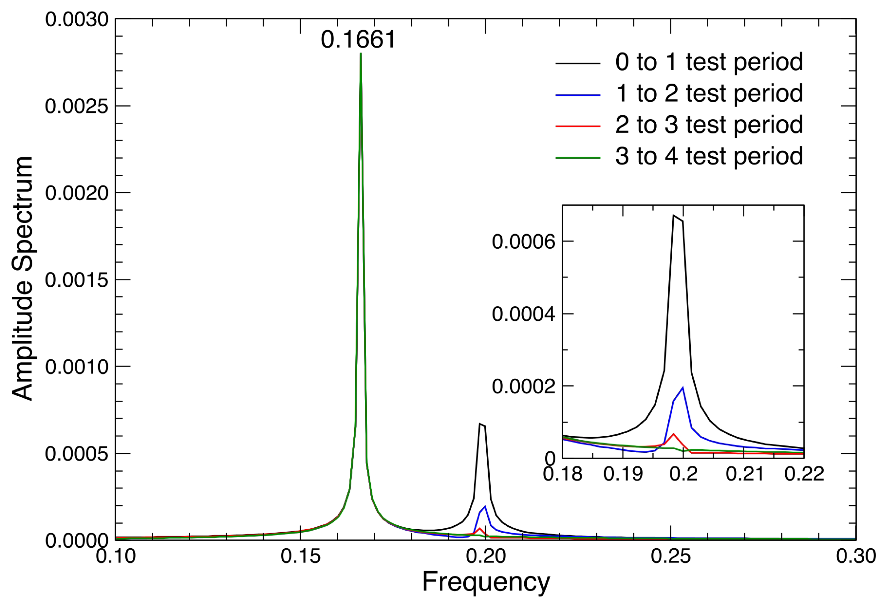
To gain more insight, a fast Fourier transformation (FFT) is applied to the time-accurate results in Figure 21 for four consecutive test periods of physical time steps, and the results of the amplitude spectrum are plotted in Figure 24. Consistent with the observations from the experiments [6], there are two dominant frequencies: the Strouhal frequency (0.1661) and the reduced structural natural frequency, (0.2), during the early transient time span of the vibration at this Reynolds number (100). One can see that the Strouhal frequency is observed for all test periods. However, the contribution of attenuates as the simulation is carried out further. As a result, initially observed non-lock-in vibration develops gradually into a lock-in VIV condition. Note that from the convergence of the VIV frequency in the One-shot analysis shown in Figure 18a, we can see that the value of fluctuates around 0.2 before dropping dramatically towards the final solution around iteration 100, implying the influence of the structural natural frequency in the development of this VIV vibration.
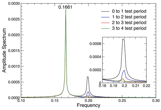
Figure 24.
Varying amplitude spectrum of time-accurate results of VIV case = 100.
4. Conclusions
In this paper, the One-shot code-coupling approach in pseudo-time was applied to a single-degree-of-freedom vortex-induced vibration system of a circular cylinder for the first time. The details of the fluid–structure coupling based on the harmonic balance technique were presented. Besides the traditionally recognized frequency lock-in (resonance) region, the HB-based One-shot method was also used to study the vibrations in non-resonant ranges of Reynolds number, and the full transition of the vibration from frequency non-lock-in to lock-in was demonstrated and analyzed, which is rarely reported in the literature. Numerical results demonstrated the high efficiency and robustness of the One-shot method, which were verified against a time-accurate method implemented in this work based on the same flow solver and the HB/LCO method as well as experimental data from the literature.
Author Contributions
H.L.: conceptualization, methodology, coding, data analysis, validation, writing—original draft and editing. K.E.: supervision, funding acquisition, resources, conceptualization, methodology, writing—review and editing. All authors have read and agreed to the published version of the manuscript.
Funding
This research was funded by the first author’s Chancellor’s Fellowship at the University of Tennessee, Knoxville, during his PhD, as well as the second author’s Fisher Professorship. The authors greatly appreciate the support provided.
Data Availability Statement
The data are contained within this article.
Conflicts of Interest
The authors declare no conflicts of interest.
Nomenclature
The following nomenclature are used in this manuscript:
| structural matrices in state-space form | |
| lift and drag coefficients, respectively | |
| pseudo-spectral matrix | |
| D | cylinder diameter |
| discrete Fourier and inverse Fourier transformation matrices, respectively | |
| flux vectors in x and y directions, respectively | |
| f | regular frequency, |
| reduced regular frequency based on cylinder diameter, | |
| structural natural frequencies of plunging in hertz (Hz) | |
| H | total enthalpy |
| h | plunge displacement |
| K | plunge stiffness of cylinder |
| L | fluid dynamic lift |
| free-stream Mach number | |
| m | mass of the plunging cylinder |
| mass ratio, | |
| N | number of harmonics |
| n | index number of harmonic mode or numerical iteration |
| p | local pressure |
| free-stream dynamic pressure, | |
| free stream Reynolds number | |
| Strouhal number, the of vortex shedding associated with the stationary cylinder | |
| s | cylinder span |
| T | plunge damping of cylinder |
| t | physical time |
| free-stream velocity | |
| conservation variables of fluid equation | |
| Fourier coefficients of conservation variables | |
| Cartesian velocity components | |
| Cartesian coordinates | |
| Z | figure-of-merit for frequency search |
| plunge coordinate damping coefficient, | |
| vector of dependent structure variables | |
| a control parameter in the cylinder VIV problem | |
| freestream kinetic viscosity | |
| local and free-stream densities, respectively | |
| vector of aerodynamic forces | |
| shear stress | |
| pseudo-time for fluid and structure solvers, respectively | |
| phase of plunging vibration | |
| angular frequency, | |
| reduced angular frequency based on cylinder diameter, | |
| structural natural frequencies of plunging, | |
| Superscripts and accents | |
| * | variable in sub-time levels (except for the mass ratio) |
| ^ | Fourier coefficients |
| · | dimensional time derivative |
| ′ | non-dimensional time derivative |
| ˜ | variable in reduced form |
| ¯ | amplitude of variable |
| Subscripts | |
| 0 | mean value |
| initial condition | |
| value at VIV condition |
References
- Williamson, C.; Govardhan, R. Vortex-induced vibrations. Annu. Rev. Fluid Mech. 2004, 36, 413–455. [Google Scholar] [CrossRef]
- Hao, Z.; Sun, C.; Lu, Y.; Bi, K.; Zhou, T. Suppression of vortex-induced vibration and phase-averaged analysis of the wake generated by a circular cylinder covered with helical grooves. Fluids 2022, 7, 194. [Google Scholar] [CrossRef]
- Wu, Y.; Lien, F.S.; Yee, E.; Chen, G. Numerical investigation of flow-induced vibration for cylinder-plate assembly at low Reynolds number. Fluids 2023, 8, 118. [Google Scholar] [CrossRef]
- Xiao, D.; Hao, Z.; Zhou, T.; Zhu, H. Experimental Studies on Vortex-Induced Vibration of a Piggyback Pipeline. Fluids 2024, 9, 39. [Google Scholar] [CrossRef]
- Cao, D.; He, J.; Zeng, H.; Zhu, Y.; Chan, S.Z.; Williams, M.R.; Khor, I.Z.L.; Yalla, O.V.; Sunny, M.R.; Ghoshal, R.; et al. A Review of Oscillators in Hydrokinetic Energy Harnessing Through Vortex-Induced Vibrations. Fluids 2025, 10, 78. [Google Scholar] [CrossRef]
- Anagnostopoulos, P.; Bearman, P. Response characteristics of a vortex-excited cylinder at low Reynolds numbers. J. Fluids Struct. 1992, 6, 39–50. [Google Scholar] [CrossRef]
- Nomura, T. Finite element analysis of vortex-induced vibrations of bluff cylinders. J. Wind. Eng. Ind. Aerodyn. 1993, 46, 587–594. [Google Scholar] [CrossRef]
- Nomura, T. ALE finite element computations of fluid-structure interaction problems. Comput. Methods Appl. Mech. Eng. 1994, 112, 291–308. [Google Scholar] [CrossRef]
- Anagnostopoulos, P. Numerical investigation of response and wake characteristics of a vortex-excited cylinder in a uniform stream. J. Fluids Struct. 1994, 8, 367–390. [Google Scholar] [CrossRef]
- Wei, R.; Sekine, A.; Shimura, M. Numerical analysis of 2D vortex-induced oscillations of a circular cylinder. Int. J. Numer. Methods Fluids 1995, 21, 993–1005. [Google Scholar] [CrossRef]
- Anagnostopoulos, P. Numerical study of the flow past a cylinder excited transversely to the incident stream. Part 1: Lock-in zone, hydrodynamic forces and wake geometry. J. Fluids Struct. 2000, 14, 819–851. [Google Scholar] [CrossRef]
- Anagnostopoulos, P. Numerical study of the flow past a cylinder excited transversely to the incident stream. Part 2: Timing of vortex shedding, aperiodic phenomena and wake parameters. J. Fluids Struct. 2000, 14, 853–882. [Google Scholar] [CrossRef]
- Bahmani, M.; Akbari, M. Effects of mass and damping ratios on VIV of a circular cylinder. Ocean. Eng. 2010, 37, 511–519. [Google Scholar] [CrossRef]
- Prasanth, T.; Premchandran, V.; Mittal, S. Hysteresis in vortex-induced vibrations: Critical blockage and effect of m. J. Fluid Mech. 2011, 671, 207–225. [Google Scholar] [CrossRef]
- Yang, F.L.; Chen, C.; Young, D. A novel mesh regeneration algorithm for 2D FEM simulations of flows with moving boundary. J. Comput. Phys. 2011, 230, 3276–3301. [Google Scholar] [CrossRef]
- Tang, G.; Lu, L.; Teng, B.; Liu, M. Numerical simulation of vortex-induced vibration with three-step finite element method and arbitrary Lagrangian-Eulerian formulation. Adv. Mech. Eng. 2013, 5, 890423. [Google Scholar] [CrossRef]
- Kaneko, S.; Hong, G.; Mitsume, N.; Yamada, T.; Yoshimura, S. Partitioned-coupling FSI analysis with active control. Comput. Mech. 2017, 60, 549–558. [Google Scholar] [CrossRef]
- Al Manthari, M.; Azeez, C.; Sankar, M.; Pushpa, B. Numerical Study of Laminar Flow and Vortex-Induced Vibration on Cylinder Subjects to Free and Forced Oscillation at Low Reynolds Numbers. Fluids 2024, 9, 175. [Google Scholar] [CrossRef]
- Ning, W.; He, L. Computation of unsteady flows around oscillating blades using linear and nonlinear harmonic Euler methods. J. Turbomach. 1998, 120, 508–514. [Google Scholar] [CrossRef]
- Hall, K.C.; Thomas, J.P.; Clark, W.S. Computation of Unsteady Nonlinear Flows in Cascades Using a Harmonic Balance Technique. AIAA J. 2002, 40, 879–886. [Google Scholar] [CrossRef]
- McMullen, M.; Jameson, A.; Alonso, J. Application of a Non-Linear Frequency Domain Solver to the Euler and Navier-Stokes Equations. In Proceedings of the 40th AIAA Aerospace Sciences Meeting & Exhibit, Reno, NV, USA, 14–17 January 2002. AIAA Paper 2002–0120. [Google Scholar] [CrossRef]
- Nadarajah, S.K. Convergence studies of the time accurate and non-linear frequency domain methods for optimum shape design. Int. J. Comput. Fluid Dyn. 2007, 21, 189–207. [Google Scholar] [CrossRef]
- Zhang, W.; Xi, G.; Zhang, C.; Huang, Z. A high-accuracy temporal–spatial pseudospectral method for time-periodic unsteady fluid flow and heat transfer problems. Int. J. Comput. Fluid Dyn. 2011, 25, 191–206. [Google Scholar] [CrossRef]
- Ekici, K.; Huang, H. An assessment of frequency-domain and time-domain techniques for turbomachinery aeromechanics. In Proceedings of the 40th AIAA Aerospace Sciences Meeting & Exhibit, New Orleans, LA, USA, 25–28 June 2012. AIAA Paper 2012-3126. [Google Scholar] [CrossRef]
- Hall, K.C.; Ekici, K.; Thomas, J.P.; Dowell, E.H. Harmonic Balance Methods Applied to Computational Fluid Dynamics Problems. Int. J. Comput. Fluid Dyn. 2013, 27, 52–67. [Google Scholar] [CrossRef]
- Carlson, H.; Feng, J.; Thomas, J.; Kielb, R.; Hall, K.; Dowell, E. Computational models for nonlinear aeroelasticity. In Proceedings of the 43rd AIAA Aerospace Sciences Meeting and Exhibit, Reno, NV, USA, 10–13 January 2005; p. 1085. [Google Scholar] [CrossRef]
- Thomas, J.P.; Dowell, E.H.; Hall, K.C. Nonlinear Inviscid Aerodynamic Effects on Transonic Divergence, Flutter, and Limit-Cycle Oscillations. AIAA J. 2002, 40, 638–646. [Google Scholar] [CrossRef]
- Kielb, R.E.; Hall, K.C.; Spiker, M.; Thomas, J.P.; Pratt, E.T., Jr.; Jeffries, R. Non-Synchronous Vibration of Turbomachinery Airfoils; Technical Report; Department of Mechanical Engineering and Materials Science, Duke University: Durham, NC, USA, 2006. [Google Scholar]
- Dowell, E.H.; Hall, K.C.; Thomas, J.P.; Kielb, R.E.; Spiker, M.A.; Denegri, C.M. A new solution method for unsteady flows around oscillating bluff bodies. In Proceedings of the IUTAM Symposium on Fluid-Structure Interaction in Ocean Engineering, Hamburg, Germany, 23–26 July 2008; Springer: Dordrecht, The Netherlands, 2008; pp. 37–44. [Google Scholar] [CrossRef]
- Spiker, M.A. Development of an Efficient Design Method for Non-Synchronous Vibrations. Ph.D. Thesis, Duke University, Durham, NC, USA, 2008. [Google Scholar]
- Clark, S.T. Design for Coupled-Mode Flutter and Non-Synchronous Vibration in Turbomachinery. Ph.D. Thesis, Duke University, Durham, NC, USA, 2013. [Google Scholar]
- Besem, F.M. Aeroelastic Instabilities due to Unsteady Aerodynamics. Ph.D. Thesis, Duke University, Durham, NC, USA, 2015. [Google Scholar]
- Besem, F.M.; Thomas, J.P.; Kielb, R.E.; Dowell, E.H. An aeroelastic model for vortex-induced vibrating cylinders subject to frequency lock-in. J. Fluids Struct. 2016, 61, 42–59. [Google Scholar] [CrossRef]
- Thomas, J.; Dowell, E. A fixed point iteration approach for harmonic balance based aeroelastic computations. In Proceedings of the AIAA Aerospace Sciences Meeting & Exhibit, Kissimmee, FL, USA, 8–12 January 2018. AIAA Paper 2018–14462018. [Google Scholar] [CrossRef]
- Blanc, F.; Roux, F.; Jouhaud, J. Harmonic-Balance-Based Code-Coupling Algorithm for Aeroelastic Systems Subjected to Forced Excitation. AIAA J. 2010, 48, 2472–2481. [Google Scholar] [CrossRef]
- Berci, M.; Dimitriadis, G. A combined Multiple Time Scales and Harmonic Balance approach for the transient and steady-state response of nonlinear aeroelastic systems. J. Fluids Struct. 2018, 80, 132–144. [Google Scholar] [CrossRef]
- Yao, W.; Jaiman, R.K. A harmonic balance technique for the reduced-order computation of vortex-induced vibration. J. Fluids Struct. 2016, 65, 313–332. [Google Scholar] [CrossRef]
- Nardini, M.; Illingworth, S.J.; Sandberg, R.D. Nonlinear reduced-order modeling of the forced and autonomous aeroelastic response of a membrane wing using Harmonic Balance methods. J. Fluids Struct. 2019, 91, 102699. [Google Scholar] [CrossRef]
- He, S.; Jonsson, E.; Mader, C.A.; Martins, J.R.R.A. A coupled Newton–Krylov time spectral solver for flutter prediction. In Proceedings of the AIAA Aerospace Sciences Meeting & Exhibit, Kissimmee, FL, USA, 8–12 January 2018. AIAA Paper 2018–2149. [Google Scholar] [CrossRef]
- He, S.; Jonsson, E.; Mader, C.A.; Martins, J. Aerodynamic Shape Optimization with Time Spectral Flutter Adjoint. In Proceedings of the AIAA Aerospace Sciences Meeting & Exhibit, San Diego, CA, USA, 7–11 January 2019. AIAA Paper 2019–0697. [Google Scholar] [CrossRef]
- He, S.; Jonsson, E.; Mader, C.A.; Martins, J.R.R.A. A Coupled Newton–Krylov Time-Spectral Solver for Wing Flutter and LCO Prediction. In Proceedings of the AIAA AVIATION Forum, Dallas, TX, USA, 17–21 June 2019. [Google Scholar]
- Maljaars, P.; Kaminski, M.; den Besten, J. A new approach for computing the steady state fluid–structure interaction response of periodic problems. J. Fluids Struct. 2019, 84, 140–152. [Google Scholar] [CrossRef]
- Ekici, K.; Hall, K.C. Harmonic Balance Analysis of Limit Cycle Oscillations in Turbomachinery. AIAA J. 2011, 49, 1478–1487. [Google Scholar] [CrossRef]
- Li, H.; Ekici, K. Revisiting the One-shot Method for Modeling Limit Cycle Oscillations: Extension to Two-degree-of-freedom Systems. Aerosp. Sci. Technol. 2017, 69, 686–699. [Google Scholar] [CrossRef]
- Li, H.; Ekici, K. Improved One-shot approach for modeling viscous transonic limit cycle oscillations. AIAA J. 2018, 56, 3138–3152. [Google Scholar] [CrossRef]
- Li, H.; Ekici, K. A novel approach for flutter prediction of pitch-plunge airfoils using an efficient One-shot method. J. Fluids Struct. 2018, 82, 651–671. [Google Scholar] [CrossRef]
- Li, H.; Ekici, K. Aeroelastic Modeling of the AGARD 445.6 Wing Using the Harmonic-Balance-Based One-shot Method. AIAA J. 2019, 57, 4885–4902. [Google Scholar] [CrossRef]
- Navrose; Mittal, S. Lock-in in vortex-induced vibration. J. Fluid Mech. 2016, 794, 565–594. [Google Scholar] [CrossRef]
- Sabino, D.; Fabre, D.; Leontini, J.; Jacono, D.L. Vortex-induced vibration prediction via an impedance criterion. J. Fluid Mech. 2020, 890, A4. [Google Scholar] [CrossRef]
- Jameson, A. A Vertex Based Multigrid Algorithm for Three Dimensional Compressible Flow Calculations. In Numerical Methods for Compressible Flows–Finite Difference, Element and Volume Techniques; AMD: New York, NY, USA, 1986; Volume 78. [Google Scholar]
- Blazek, J. Computational Fluid Dynamics: Principles and Applications; Butterworth-Heinemann: Oxford, UK, 2015. [Google Scholar]
- Jameson, A.; Schmidt, W.; Turkel, E. Numerical Solution of the Euler Equations by Finite Volume Methods Using Runge-Kutta Time Stepping Schemes. In Proceedings of the AIAA Aerospace Sciences Meeting & Exhibit, St. Louis, MO, USA, 12–15 January 1981. AIAA Paper 81–1259. [Google Scholar] [CrossRef]
- Jameson, A. Solution of the Euler Equations for Two Dimensional Transonic Flow by a Multigrid Method. Appl. Math. Comput. 1983, 13, 327–355. [Google Scholar] [CrossRef]
- Huang, H.; Ekici, K. Stabilization of high-dimensional harmonic balance solvers using time spectral viscosity. AIAA J. 2014, 52, 1784–1794. [Google Scholar] [CrossRef]
- Chorin, A.J. A numerical method for solving incompressible viscous flow problems. J. Comput. Phys. 1997, 135, 118–125. [Google Scholar] [CrossRef]
- Ekici, K.; Hall, K.C. Nonlinear analysis of unsteady flows in multistage turbomachines using harmonic balance. AIAA J. 2007, 45, 1047–1057. [Google Scholar] [CrossRef]
- Nimmagadda, S.; Economon, T.D.; Alonso, J.J.; da Silva Ilario, C.R. Robust uniform time sampling approach for the harmonic balance method. In Proceedings of the AIAA Aerospace Sciences Meeting & Exhibit, San Diego, CA, USA, 4–8 January 2016. AIAA Paper 2016–3966. [Google Scholar] [CrossRef]
- Li, H. The One-shot Aeroelastic Method: A Highly Efficient Modeling Approach Based on the Harmonic Balance Technique. Ph.D. Thesis, University of Tennessee, Knoxville, TN, USA, 2019. [Google Scholar]
- Li, H.; Ekici, K. Supplemental-frequency harmonic balance: A new approach for modeling aperiodic aerodynamic response. J. Comput. Phys. 2021, 436, 110278. [Google Scholar] [CrossRef]
- Williamson, C.H. Defining a universal and continuous Strouhal–Reynolds number relationship for the laminar vortex shedding of a circular cylinder. Phys. Fluids 1988, 31, 2742–2744. [Google Scholar] [CrossRef]
- Tanida, Y.; Okajima, A.; Watanabe, Y. Stability of a circular cylinder oscillating in uniform flow or in a wake. J. Fluid Mech. 1973, 61, 769–784. [Google Scholar] [CrossRef]
- Keefe, R.T. Investigation of the fluctuating forces acting on a stationary circular cylinder in a subsonic stream and of the associated sound field. J. Acoust. Soc. Am. 1962, 34, 1711–1714. [Google Scholar] [CrossRef]
- Djeddi, R.; Ekici, K. Resolution of Gibbs phenomenon using a modified pseudo-spectral operator in harmonic balance CFD solvers. Int. J. Comput. Fluid Dyn. 2016, 30, 495–515. [Google Scholar] [CrossRef]
- Norberg, C. Flow around a circular cylinder: Aspects of fluctuating lift. J. Fluids Struct. 2001, 15, 459–469. [Google Scholar] [CrossRef]
- He, T.; Zhou, D.; Bao, Y. Combined interface boundary condition method for fluid–rigid body interaction. Comput. Methods Appl. Mech. Eng. 2012, 223, 81–102. [Google Scholar] [CrossRef]
- He, T.; Zhou, D.; Han, Z.; Tu, J.; Ma, J. Partitioned subiterative coupling schemes for aeroelasticity using combined interface boundary condition method. Int. J. Comput. Fluid Dyn. 2014, 28, 272–300. [Google Scholar] [CrossRef]
- He, T.; Zhang, K.; Wang, T. AC-CBS-based partitioned semi-implicit coupling algorithm for fluid-structure interaction using stabilized second-order pressure scheme. Commun. Comput. Phys. 2017, 21, 1449–1474. [Google Scholar] [CrossRef]
- Williamson, C.H.; Roshko, A. Vortex formation in the wake of an oscillating cylinder. J. Fluids Struct. 1988, 2, 355–381. [Google Scholar] [CrossRef]
- Nestor, R.M.; Quinlan, N.J. Application of the meshless finite volume particle method to flow-induced motion of a rigid body. Comput. Fluids 2013, 88, 386–399. [Google Scholar] [CrossRef]
- Bahmani, M.; Akbari, M. Response characteristics of a vortex-excited circular cylinder in laminar flow. J. Mech. Sci. Technol. 2011, 25, 125–133. [Google Scholar] [CrossRef]
- Geuzaine, P.; van der Zee, K.; Farhat, C. Second-Order Time-Accurate Loosely-Coupled Solution Algorithms for Nonlinear FSI Problems. In Proceedings of the European Congress on Computational Mechanics in Applied Sciences and Engineering, Barcelona, Spain, 20–25 July 2004. [Google Scholar]
- He, T. On the mesh insensitivity of the edge-based smoothed finite element method for moving-domain problems. Comput. Methods Appl. Mech. Eng. 2025, 440, 117917. [Google Scholar] [CrossRef]
- Dettmer, W.; Perić, D. A computational framework for fluid–rigid body interaction: Finite element formulation and applications. Comput. Methods Appl. Mech. Eng. 2006, 195, 1633–1666. [Google Scholar] [CrossRef]
- Tan, W.; Wu, H.; Zhu, G. Fluid-structure interaction using Lattice Boltzmann method: Moving boundary treatment and discussion of compressible effect. Chem. Eng. Sci. 2018, 184, 273–284. [Google Scholar] [CrossRef]


Disclaimer/Publisher’s Note: The statements, opinions and data contained in all publications are solely those of the individual author(s) and contributor(s) and not of MDPI and/or the editor(s). MDPI and/or the editor(s) disclaim responsibility for any injury to people or property resulting from any ideas, methods, instructions or products referred to in the content. |
© 2025 by the authors. Licensee MDPI, Basel, Switzerland. This article is an open access article distributed under the terms and conditions of the Creative Commons Attribution (CC BY) license (https://creativecommons.org/licenses/by/4.0/).