Abstract
The dam break flow problem consists of the phenomena where a fluid is suddenly released and is often used as a test case for multiphase flows numerical models or to analyze the underlying physics of complex free surface flows of both Newtonian and non-Newtonian fluids. Dam break flows of viscoplastic fluids (i.e., fluids that present a yield stress) are especially interesting for two reasons: many geological and industrial fluids can be characterized as viscoplastic fluids, and the yield stress represents a difficulty for numerical solutions. The viscoplastic fluids are simulated using the Bingham and Herschel–Bulkley models, and the results are compared with the flow development of power-law and Newtonian fluids (i.e., with no yield stress). This paper focuses on the numerical modeling of viscoplastic two-dimensional dam-break flows on an inclined bed as a means to analyze the shear stress field development over time and the formation of plug and pseudo-plug zones. It is shown that, for the very beginning of flow, the yield stress fluids were characterized by three distinctive shear stress zones, an occurrence that could not be found on the fluid with no yield stress.
1. Introduction
Naturally occurring flows, such as landslides, debris flows, snow avalanches and several geological flows, as well as man induced flows, for example, in the occurrence of tailing dam breaks, share important characteristics: under certain circumstances it is convenient to describe these as non-Newtonian dam break flows [1,2,3,4,5]. One key aspect of these flows is the disastrous effects on downstream regions that can be produced [6,7,8]. The fast transient behavior of dam break flows also makes it a problem prototype commonly used as a benchmark case for the analysis of numerical modeling of multiphase flows [9,10,11].
There is a vast quantity of geological flows that present non-Newtonian behavior, and the literature presents a wide variety of rheological models to describe them [12,13,14,15,16,17]. This work focuses on the dam break flow of viscoplastic shear thinning and shear thickening fluids. Viscoplastic fluids are characterized by the occurrence of a critical yielding value below which the fluid presents, at least in a macroscopic perspective, a solid-like behavior (the microscopic study of viscoplastic geological fluids is discussed in [16,18,19,20]).
The majority of viscoplastic geological fluids are characterized as yield stress shear thinning fluids [18,21]. This category includes mud flows, snow avalanches and muddy debris flows, i.e., with small concentrations of thicker solids, as proposed by the classification of Coussot and Meunier [13]. Even though it is not common to find dilatant fluids in geological flows, there is evidence that granular debris and highly concentrated suspension flows behave as shear thickening fluids [21,22,23,24]. Nonetheless, it is important to highlight that, with the increase in solid particle concentration, the suitability of rheology models to describe these problems may be inadequate. It is suggested that for these situations the interparticle force modeling plays a strong part in the description of the macroscopic behavior of the fluids [14,23,24,25].
Free surface flows in general are commonly modeled by simplified theories that do not require the calculation of the gaseous phase. Lubrication, kinetic waves and shallow water theories are some of the most common types of simplified models [1,2,3,4,5,15,23,25,26,27,28,29,30]. Real geological events use these simplified theories to offset the enormous (and sometimes prohibitive) computational costs of full multiphase flow models. Nonetheless, some clarification on these flow dynamics still needs to be addressed. For example, the existence of a yield stress results in the creation of a region of elastic solid-like behavior and a region of plastic behavior. The use of yield stress models is controversial, however, it is very convenient to deal with the inherent complexities of these fluids [16,17]. Ancey and Chochard [5] show that the local mean values used on shallow water solutions leads to the existence of a continuous yield surface along the flow direction. Nonetheless, for gradually varying mild slopes, fluids that present yield stress arguably produce an unsheared zone (or plug zone) confined to the free surface of the downstream region. The work of Piau [6] also indicates that the normal stress contribution should not be neglected.
Balmforth and Craster [26] argue that considering the free surface to be a stress-free surface would prohibit the flow from having a true plug zone near the surface. This gives rise to the pseudo-plug region concept, i.e., regions that only appear to be unsheared. Another conclusion of this work is that the plug zones appear naturally on previous shallow water and similar mathematical models (such as the lubrication theory) caused by the non-inclusion of O(ε) terms (where ε is the flow aspect ratio). This conclusion was confirmed by Fernádez-Nieto et al. [25] and Chambon [31]. Yet, it is possible the appearance of true plug zones inside pseudo-plugs.
Regarding the numerical solution of viscoplastic fluids flows, Balmforth et al. [16] point to the difficulty in reproducing the solid, rigid structure of true plug zones and tracking the yield surfaces. The authors point out two main ways to obtain the yield surface positions: augmented Lagragian methods (based on a variational formulation of the Navier-Stokes equations) and the use of regularized constitutive relations. One key aspect of the work is that the Lagrangean approach can describe the velocity fields more accurately but has difficult implementation strategies and higher computational cost. The use of unconventional approaches, such as the Lattice Boltzmann method [28], has questionable capacity in adequately modeling the bottom shear stress in shallow water solutions for the Herschel–Bulkley fluids [16].
This paper focuses on the numerical modeling of viscoplastic dam-break flows to analyze the shear stress field development over time. The results can be used for the validation of real-life problem numerical solutions, as well as to develop insights into the creation of new shallow water models and other approximated theories. The Herschel–Bulkley model (HB) is used as the main operating fluid due to its generalized Newtonian formulation that handles not only yield stress fluids but also shear thinning and shear thickening ones; this solution is compared to dam break flows results with Bingham plastics and Newtonian fluids.
2. Problem Description
The benchmark problem considered in this work is the two-dimensional dam break of a non-Newtonian reservoir fluid down an inclined channel, as shown in Figure 1. The solution domain consists of a closed two-dimensional box, where all the boundary conditions for the problem are a no-slip condition for all walls.
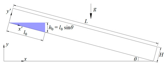
Figure 1.
Geometry of the two-dimensional dam break flow down an inclined channel.
The fluid motion (non-Newtonian liquid and air) is governed by the mass and momentum conservation equations for incompressible flows, Equations (1) and (2):
where is the velocity vector; is the identity matrix; is the shear stress tensor; is the strain rate tensor, and is the apparent viscosity (equal to the dynamic viscosity in case of Newtonian fluids).
The Herschel–Bulkley model establishes that:
where is the yield stress; is called flow index, is the consistency index, and is the second invariant of the strain rate tensor.
Shear thinning and shear thickening fluids are modeled, respectively, with and . Equation (3) can retrieve the apparent viscosity of Power law fluids by making ; Bingham plastics can be obtained by making and Newtonian fluids by making and (and, in this case, is equal to dynamic viscosity).
3. Materials and Methods
Free surface problems (essentially two-phase flows) can be numerically solved by several approaches [32]. The Volume of Fluid—VOF method, selected for this work, uses a whole domain approach, solving Equations (4) and (5) using the gas volumetric fraction to proportionally calculate the thermophysical properties throughout the numerical solution domain. This volumetric fraction is denoted by and varies between values 0 (for a cell that contains only gas) and 1 (for a cell that contains no gas), and this enforces a unitary sum of volumetric fractions for each cell:
where represents the gas phase, and represents the liquid phase.
To efficiently use this whole domain formulation an additional equation for the volumetric fraction needs to be solve, and this is accomplished using an advection equation for the phase fractions. As there are two phases in this problem, only one phase equation must be solved, in the case of the simulation in this work the equation for the gas phase was chosen to be solved as indicated in Equation (5), while the liquid volumetric fraction is calculated using the volumetric restriction equation represented by Equation (4).
The thermophysical properties are then calculated for each cell using a proportional average between the phases that occupy each cell:
The interface between phases can be reconstructed using different methods [9,11], and the result of this procedure is used to update the volume fraction field by solving Equation (5) with the converged velocity field from Equation (2). The geometric reconstruction method (Piecewise Linear Interface Calculation—PLIC method) generally presents the best results [11] and is selected for this work.
The software Ansys Fluent 2023-R2 is used for the simulations of a two-dimensional channel, as presented in Figure 1, with length L = 2000 mm and height H = 200 mm, in four distinct inclinations (θ = 5°, 10°, 15° and 20°). All simulations were performed with l0 = 500 mm and a regular mesh of 100,000 cells. The time step values were set between 50 and 1000 µs depending on the case to ensure convergence (the use of a uniform time step would have been prohibitive due to high computational costs); time integration was performed with the only available option in Ansys Fluent, the First Order Euler Integration. The densities of the non-Newtonian fluid and of the air are, respectively, set to 1000 kg/m3 and 1.8 kg/m3; gravity is considered 9.81 m/s2 in all cases, and all simulations were performed until time equal to 5 s. The viscosity of air is considered constant and equal to 18.5 µPa.s. The interaction between phases in the sense of surface forces is neglected due to the unavailability of surface tension and contact angle data for the range of fluid properties used in this work.
The hypothetical fluids used are listed in Table 1 (totaling 32 simulations) along with all relevant rheological parameters.

Table 1.
Rheological parameters of the simulated fluids.
The existence of yield stress creates infinity viscosities at a zero shear rate and are difficult to overcome. One strategy to deal with this characteristic is to use regularization models. Mitsoulis and Tsamopoulos [17], and Frigaard and Nouar [33], presented reviews on this subject and supported the work presented here; these works also highlight that all regularization methods rely on one or more adjustable parameters to limit the values of apparent viscosity to be finite.
This work uses the following model [10] and applies the guidelines presented in Inacio et al. [34] for the regularization parameters:
where , is an inferior limit of and is a superior limit of . For all simulations the limits used are: and (a value much higher than those found in the simulations). The same authors indicate that the most adequate method to obtain the yield surface is to investigate shear stress contours, as is done in this work. It is important to explain that, from this moment on, when the text refers to shear stress, it must be understood that it is referring to the second invariant of the tensor, .
The results presented in the following section are analyzed in terms of the Froude and Reynolds (modified for Herschel–Bulkley fluids [1]) numbers, as defined in Equations (8) and (9); the area averaged shear stress and the base wall (bed) shear stress, .
where is the mean longitudinal velocity for the cross-sectional area under analysis and is the perpendicular distance from the bottom wall (floor) to the interface. The Reynolds number for Herschel–Bulkley fluids is usually calculated by the following expression.
4. Results and Discussions
One key aspect in presenting results for the immiscible multiphase flow is the determination of the interface position. The VOF model was developed to produce sharp, line-like interfaces, however, as it is common to all approximate solutions, the phenomenon of numerical diffusion is inevitably present. This problem is well documented in the literature (Barral et al. [9]), and for the scope of this paper the interface position is defined as a volume fraction contour of α = 0.5. This mitigates the displaying of numerical diffusion at the interface, eliminating the smearing caused by it. It is necessary to highlight that the numerical diffusion is still present in the simulations if it occurred in the way demonstrated by Barral et al. [9], however, it does not get displayed in results, allowing for a clear view and interpretation of the flow.
Numerical diffusion is a spurious phenomenon that has been plaguing numerical solutions of physical and engineering problems with elevated gradients since the inception of the Finite Volumes Method, as the first concise discussion about it is presented by Patankar [35]. Although much has been done to improve the treatment of high gradient problems numerical solutions, and to some extent its detrimental effect has been mitigated, as is evident from Maliska [36], Veersteeg and Malalasekeera [37], and Barral et al. [9], this is still a concern with this type of problem, acting as a smoother of the real gradient. This artificial smoothing of the interface is present in all VOF simulations, as demonstrated by Barral et al. [9] and dos Santos et al. [11], so using a fixed interface volumetric fraction avoids displaying this as a real result.
Figure 2 shows the interface position over time (t = 0.2 s; 0.5 s; 1.0 s; 1.5 and 2.0 s) for θ = 5° and 20°. The omitted time steps represent the cases that have a complete fluid flow, with the interface reaching the end of the channel (for example, Fluid 1 reaches the channel end in the θ = 20° case between 0.5 and 1.0 s). Of all test cases the only scenario that did not reach full development of the flow front is the case for the slope of θ = 5° and Fluid 2. Common sense dictates that the onset of the flow is controlled by the relation between the pressure on the fluid interface at the base of the reservoir and the yield stress [1], and this leads to the fluid motion starting at a pressure higher than that, indicating a minimum value of the initial height [38] as:
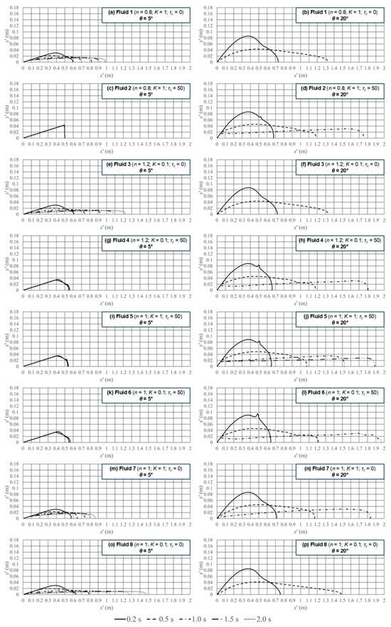
Figure 2.
Time evolution of the interface for two different slopes and fluids.
As yield stress was kept constant for all yield stress fluids, it follows that the minimum height required for motion to initiate depends only on the channel slope. Table 2 resumes the initial and the minimum heights.
Table 2.
Initial high and minimum high for the yield stress fluids to initiate flow.
From this perspective, all fluids with yield stress (Fluids 2, 4, 5 and 6) should remain motionless, not experiencing any kind of flow for the 5° channel inclination. The reason for the presence of movement in Fluids 4, 5 and 6, even with an initial height lower than the minimum, is that Equation (10) does not account for the use of a regularization method that smooths the behavior of shear stress for very low strain rates. Nonetheless, it is inconclusive why Fluid 5 presented an initial flow, while Fluid 2 remained stationary, because Fluid 5 presents a higher value of flow index (n).
This arrested state could also be analyzed in terms of balance of forces [5]. For steep slopes, the balance is theorized to happen between gravitational and viscous forces, and for nearly horizontal channels between pressure cross flow gradient and viscosity. Such analysis is left for possible future work.
Figure 3 shows the wave front position over time marked as the position of the interface contact with the lower wall of the domain (channel bed). One direct observation of this is that only the yield stress fluids achieve an arrested state (stopping the motion) that is characterized by the occurrence of a plateau in the interface position. These results show an apparent discrepancy for the interface evolution of Fluid 1 in the 5° slope channel: between 0.4 and 0.7 s the interface apparently oscillates, presenting a smaller distance in a later time. This phenomenon is probably due to the previously mentioned occurrence of interfacial smearing caused by numerical diffusion. These results allow for an observation of the interfacial velocity change as the flow progresses, and of the deceleration induced by the presence of the yield stress in Fluids 2, 4, 5, and 6. Fluids 2, 4, and 6 also present some interesting behavior on the wave front—an apparent inflection point. The occurrence of this implies that the weight of the undeformed fluid above the shearing layer reaccelerates the bulk motion, forcing the fluid to flow for a longer time.
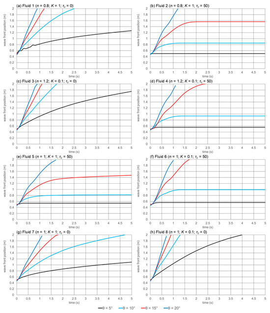
Figure 3.
Front wave time evolution for different slopes and fluids.
Figure 4 and Figure 5 show the velocity and shear stress fields for 0.1 s, while Figure 6 and Figure 7 show the same results for 0.5 s. The figures were zoomed in for a better visualization of the results. The shear stress fields were divided into two color schemes. One for stresses smaller than 50 Pa (even for the fluid with no yield stress) and the other one for stresses higher than that value.
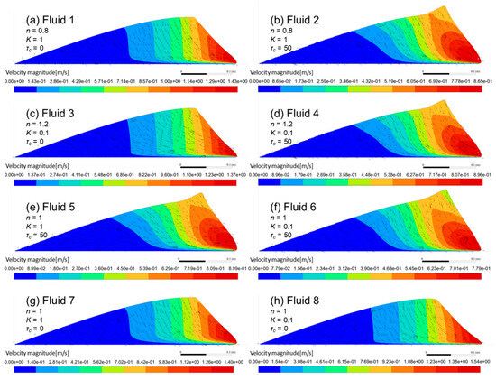
Figure 4.
Velocity fields for t = 0.1 s and θ = 20°.
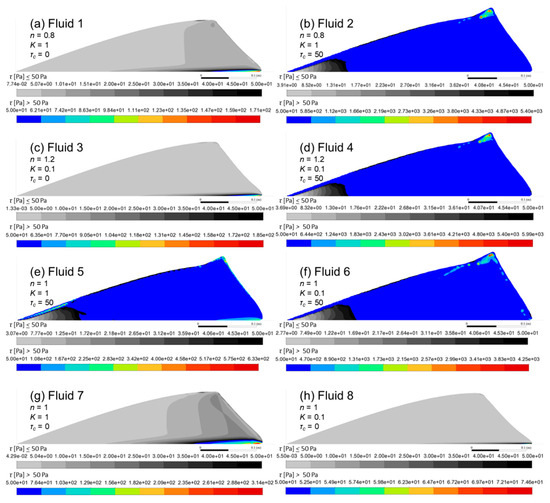
Figure 5.
Shear stress fields for t = 0.1 s and θ = 20°.
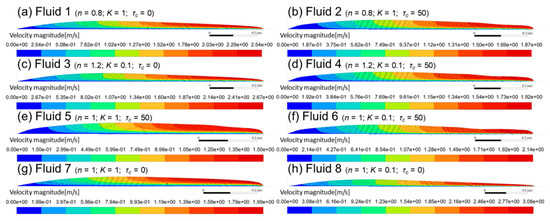
Figure 6.
Velocity fields for t = 0.5 s and θ = 20°.
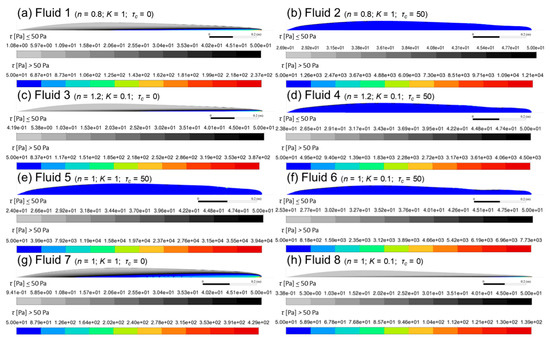
Figure 7.
Shear stress fields for t = 0.5 s and θ = 20°.
The analysis of the shear stress field for the yield stress fluids (shown in Figure 8) reveals a common configuration during the initial phase of the flow (0.1 s), a significant portion of shear stresses approaches the fluid’s yield value (zone 1); sheared fluid patches (zone 2) appear on the backside of the free surface near the beginning of the channel, the wave crest and bottom of the wave front near the channel wall; and an unsheared zone also appears (zone 3). No meaningful difference was detected for different values of k and n. For the fluid with no yield stress, there were only two zones: the first one included most of the fluid and presented small shear stress values, while the second one was restricted to small regions near the wall and presented the higher values for shear stresses. This difference between fluid with no yield stress and yield stress fluids seems to be the reason for the almost linear growth of the velocity magnitudes from downstream to upstream, in contrast with the velocity field growth found on the yield stress fluids. It also should be highlighted that the unsheared zone rapidly disappears (Figure 7) with no identifiable parts of the yield stress fluids presenting < . In fact, almost all yield stress fluids present values just above the value, and only by a very small margin.
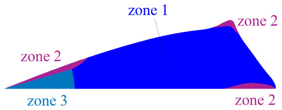
Figure 8.
Generic shear stress field zones for the yield stress fluids and t = 0.1 s and θ = 20°.
Minussi and Maciel [10] used a value of 10−3 1/s for the shear stress inferior limit, which proved to be a good choice after the comparison with the experimental results and the deformation rates found for the problem. This work followed the same guidelines for the rheological parameters that allow for the deformation rates developed to be the same orders of magnitude as this previous work. Viscoplastic models lead to infinite viscosities for stresses lower those of critical stress, and the use of regularized models requires small values so that the viscosity behavior is close to the original models. Therefore, it was decided to adopt a value 10 times smaller than that used in Minussi and Maciel [10].
It is important to remember that viscoplastic models such as those of Bingham and Herschel–Bulkley do not include any type of deformation for stresses lower than the critical one. When using a regularization model, small deformations will obviously occur, but such deformations can be considered unphysical. For this reason, it is important to emphasize that the regions represented in Figure 8 as unsheared zones (zone 3) are not, in fact, unsheared zones but rather zones with stresses lower than the critical ones and can therefore be more conveniently called pseudo-plug zones. It should also be clear that the absence of true plug zones does not corroborate results using shallow water models since the Navier–Stokes model used here is not limited to the condition of zero surface stresses, as pointed out by Ancey and Cochard [5], and Balmforth and Craster [26]. One way to verify the existence of true plug zones would be to include viscoelastic effects and/or use augmented Lagrangian methods (Balmforth et al. [16]).
Figure 9 presents the time evolution of shear stress averaged values (calculated as averaged values over the whole fluid domain) and bed shear stress (calculated as area averaged over the bottom wall). It is necessary to highlight that the maximum values for both parameters happen between 0.9 and 1.5 s after fluid release with no noticeable difference between yield and fluid with no yield stress. The instantaneous values for bed shear stress are up to 20 times higher than those of averaged shear stress, with the curves presenting the similar temporal behavior. This is an indication that for all fluids, the higher shear stresses occur at the bottom of the liquid, as expected. Figure 9 also reveals that it is not possible to correlate the formation of the shear stress field zones (from Figure 8) with either the shear stress averaged values or the bed shear stress. For the cases where the fluids reached the channel end before 2 s, Figure 9 also indicates the approximated impact time with the end channel wall (displayed as vertical green, red and blue lines). This also reveals an unchanged overall behavior of and for all cases, indicating smooth sloshing flow.
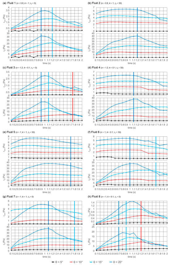
Figure 9.
Time values of volumetric averaged value of the shear stress inside each fluid and area averaged value of the bed shear stress. The vertical lines show the approximated instant of impact with the downstream channel wall.
Figure 10 shows the values of Froude, Fr, and Reynolds number (modified for Herschel–Bulkley fluids), Re; calculated for three cross sections (plane 1 for x′ = 0.5 m; plane 2 for x′ = 0.75 m and plane 3 for x′ = 1.0 m). It can be verified that the laminar flow simplification (for free surface flow Re < 500) is satisfied for all cases and that all flows are subcritical (Fr < 1). Nonetheless, the overall behavior of the Froude number is consistent with those of Muchiri et al. [30], with the Froude number being reduced downstream. However, it was not possible to observe the decrease in the Froude number with the increase in the index number, as found by Muchiri et al. [30]; this last observation is likely to be caused by the different index number ranges used by each work.
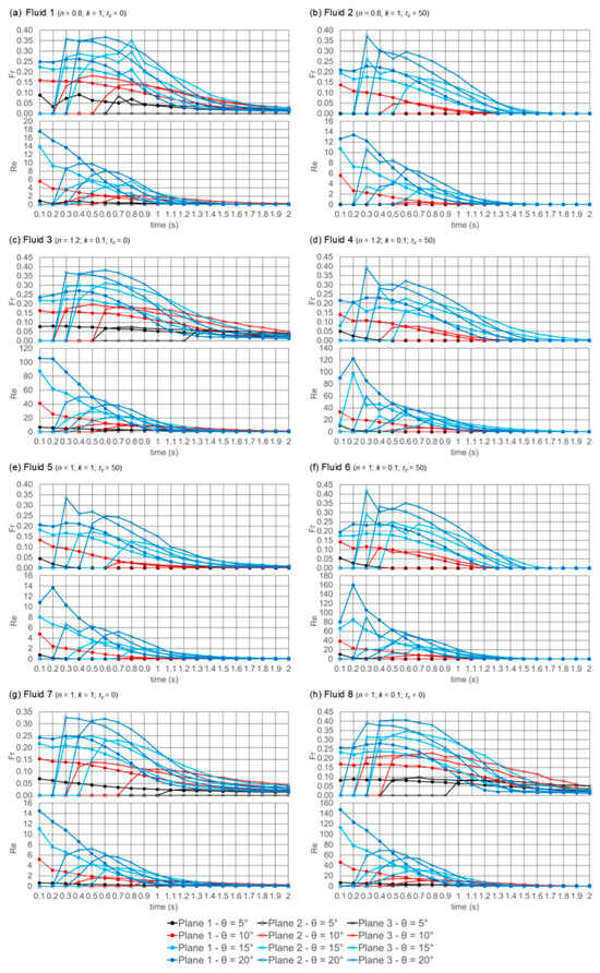
Figure 10.
Time evolution of Fr and Re values for Planes 1 (x′ = 0.5 m); 2 (x′ = 0.75 m) and 3 (x′ = 1 m).
5. Conclusions
This paper was concerned with the numerical analysis of the shear stress field and the formation of plug and sheared zones on the dam break flows of viscoplastic fluids. Eight hypothetical fluids were simulated with different values of flow and consistency indexes and two values of yield stress. The results revealed a common configuration of the shear stress field for all the yield stress fluids, as opposed to the shear stress field of the fluid with no yield stress. The viscoplastic fluids presented the formation of plug zones at the very beginning of the flow, a phenomenon that could not be observed on the fluid with no yield stress. These plug zones disappeared rapidly with the flow development, however, with consequences on the wave front position and velocity magnitudes over time. No meaningful difference was detected for different values of the used consistency and flow indexes, a result that requires further investigation of different values of those indexes.
It is important to highlight that the presented results are only valid to isotropic viscoplastic fluids with no thixotropic behavior. Therefore, the results found herein do not account for any elastic or anisotropic behavior, such as the ones that can be found on some types of clay materials submitted to overconsolidation [39]. Another limitation is due to the two-dimensional formulation that cannot represent some phenomena such as lateral levees [5] and fingering instabilities [27]. Despite these limitations, it is hoped that the presented results can be used for the validation of real-life engineering problems, as well to develop insights into the creation of new shallow water models and other approximated theories. For future endeavors, we hope to analyze other hypothetical fluids with different values of consistency and flow indexes, and the usage of different regularization methods. The comparison with experimental results and the implementation of three-dimensional simulations is also expected to be conducted.
Author Contributions
R.B.M. contributed to the conceptualization, simulations post-processing, the formal analysis, and writing. M.V.C.A. contributed to the simulation setup and running, the formal analysis, and writing. G.d.F.M. helped with the formal analysis and writing. All authors contributed to funding acquisition. All authors have read and agreed to the published version of the manuscript.
Funding
The authors wish to thank for the financial support of the “Fundação da Universidade Federal do Paraná (FUNPAR)”, through concession FDA 2021-Project 03748; to the “Fundação de Amparo à Pesquisa e Inovação do Estado de Santa Catarina (FAPESC)”, through concessions FAPESC 2019TR000779, 2019TR000783, 2019TR000843, 2021TR000843 and 2023TR000563; to the “Conselho Nacional de Desenvolvimento Científico e Tecnológico (CNPq)”, through concession CNPq 433820/2018-7; and to the “Coordenação de Aperfeiçoamento de Pessoal de Nível Superior (CAPES)” through Code 001 and to the “Fundação de Amparo à Pesquisa do Estado de São Paulo” through concession APR 2020/07822-0.
Data Availability Statement
The original contributions presented in this study are included in the article. Further inquiries can be directed to the corresponding author.
Conflicts of Interest
The authors have no conflicts of interest to declare that are relevant to the content of this article.
References
- Huang, X.; García, M.H. A Herschel–Bulkley model for mud flow down a slope. J. Fluid Mech. 1998, 374, 305–333. [Google Scholar] [CrossRef]
- Chanson, H.; Jarny, S.; Coussot, P. Dam Break Wave of Thixotropic Fluid. J. Hydraul. Eng. 2006, 132, 280–293. [Google Scholar] [CrossRef][Green Version]
- Balmforth, N.; Craster, R.; Perona, P.; Rust, A.; Sassi, R. Viscoplastic dam breaks and the Bostwick consistometer. J. Non-Newton. Fluid Mech. 2007, 142, 63–78. [Google Scholar] [CrossRef]
- Matson, G.; Hogg, A. Two-dimensional dam break flows of Herschel–Bulkley fluids: The approach to the arrested state. J. Non-Newton. Fluid Mech. 2007, 142, 79–94. [Google Scholar] [CrossRef]
- Ancey, C.; Cochard, S. The dam-break problem for Herschel–Bulkley viscoplastic fluids down steep flumes. J. Non-Newton. Fluid Mech. 2009, 158, 18–35. [Google Scholar] [CrossRef]
- Piau, J. Flow of a yield stress fluid in a long domain. Application to flow on an inclined plane. J. Rheol. 1996, 40, 711–723. [Google Scholar] [CrossRef]
- Coussot, P.; Laigle, D.; Arattano, M.; Deganutti, A.; Marchi, L. Direct determination of rheological characteristics of debris flow. J. Hydraul. Eng. 1998, 124, 865–868. [Google Scholar] [CrossRef]
- Li, X.; Zhao, J. Dam-break of mixtures consisting of non-Newtonian liquids and granular particles. Powder Technol. 2018, 338, 493–505. [Google Scholar] [CrossRef]
- Barral, A.A., Jr.; Minussi, R.B.; Canhoto Alves, M.V. Comparison of Interface Description Methods Available in Commercial CFD Software. J. Appl. Fluid Mech. 2019, 12, 1801–1812. [Google Scholar] [CrossRef]
- Minussi, R.B.; Maciel, G.d.F. Numerical experimental comparison of dam break flows with non-Newtonian fluids. J. Braz. Soc. Mech. Sci. Eng. 2012, 34, 167–178. [Google Scholar] [CrossRef]
- Santos, K.M.O.; Minussi, R.B.; Alves, M.V.C. Evaluation of the Level-Set and Anti-Diffusion Functions Influence in the Simulation of Non-Newtonian Dam Break Problems. In Engineering Design Applications VI—Structures, Materials and Processes; Springer: Berlin/Heidelberg, Germany, 2024. [Google Scholar]
- Perzyna, P. The Study of the Dynamic Behavior of Rate Sensitive Plastic Materials; Division of Applied Mathematics, Brown University: Providence, RI, USA, 1962. [Google Scholar]
- Coussot, P.; Meunier, M. Recognition, classification and mechanical description of debris flows. Earth-Sci. Rev. 1996, 40, 209–227. [Google Scholar] [CrossRef]
- Ancey, C. Plasticity and geophysical flows: A review. J. Non-Newton. Fluid Mech. 2007, 142, 4–35. [Google Scholar] [CrossRef]
- Saramito, P.; Smutek, C.; Cordonnier, B. Numerical modeling of shallow non-Newtonian flows: Part I. The 1D horizontal dam break problem revisited. Int. J. Numer. Anal. Model. B 2013, 4, 283–298. [Google Scholar]
- Balmforth, N.J.; Frigaard, I.A.; Ovarlez, G. Yielding to stress: Recent developments in viscoplastic fluid mechanics. Annu. Rev. Fluid Mech. 2014, 46, 121–146. [Google Scholar] [CrossRef]
- Mitsoulis, E.; Tsamopoulos, J. Numerical simulations of complex yield-stress fluid flows. Rheol. Acta 2017, 56, 231–258. [Google Scholar] [CrossRef]
- Rakshith, S.; Zhang, X.; Coussot, P.; Singh, D.N. Complex-Fluid Approach for Determining Rheological Characteristics of Fine-Grained Soils and Clay Minerals. J. Mater. Civ. Eng. 2018, 30, 04018322. [Google Scholar] [CrossRef]
- Jeon, C.-H.; Hodges, B.R. Comparing thixotropic and Herschel–Bulkley parameterizations for continuum models of avalanches and subaqueous debris flows. Nat. Hazards Earth Syst. Sci. 2018, 18, 303–319. [Google Scholar] [CrossRef]
- Christophe, A.; Neil, B.; Ian, F. Editorial—Visco-plastic fluids: From Theory to Application. J. Non-Newton. Fluid Mech. 2009, 158, 3. [Google Scholar]
- Maciel, G.d.F.; dos Santos, H.K.; Ferreira, F.d.O. Rheological analysis of water clay compositions in order to investigate mudflows developing in canals. J. Braz. Soc. Mech. Sci. Eng. 2009, 31, 64–74. [Google Scholar] [CrossRef]
- Takahashi, T. Debris Flow: Mechanics, Prediction, and Countermeasures, 2nd ed.; CRC Press: Boca Raton, FL, USA, 2014; 551p, ISBN 9781138000070. [Google Scholar]
- Iverson, R.M.; Denlinger, R.P. Flow of variably fluidized granular masses across three-dimensional terrain: 1. Coulomb mixture theory. J. Geophys. Res. Solid Earth 2001, 106, 537–552. [Google Scholar] [CrossRef]
- Balmforth, N.; Craster, R. Geophysical aspects of non-Newtonian fluid mechanics. In Geomorphological Fluid Mechanics; Springer: Berlin/Heidelberg, Germany, 2001; pp. 34–51. [Google Scholar]
- Fernández-Nieto, E.; Garres-Díaz, J.; Vigneaux, P. Multilayer models for hydrostatic Herschel-Bulkley viscoplastic flows. Comput. Math. Appl. 2023, 139, 99–117. [Google Scholar] [CrossRef]
- Balmforth, N.; Craster, R. A consistent thin-layer theory for Bingham plastics. J. Non-Newton. Fluid Mech. 1999, 84, 65–81. [Google Scholar] [CrossRef]
- Nsom, B.; Debiane, K.; Piau, J.-M. Bed slope effect on the dam break problem. J. Hydraul. Res. 2000, 38, 459–464. [Google Scholar] [CrossRef]
- Ancey, C.; Andreini, N.; Epely-Chauvin, G. Viscoplastic dambreak waves: Review of simple computational approaches and comparison with experiments. Adv. Water Resour. 2012, 48, 79–91. [Google Scholar] [CrossRef]
- Andreini, N.; Epely-Chauvin, G.; Ancey, C. Internal dynamics of Newtonian and viscoplastic fluid avalanches down a sloping bed. Phys. Fluids 2012, 24, 053101. [Google Scholar] [CrossRef]
- Muchiri, D.K.; Hewett, J.N.; Sellier, M.; Moyers-Gonzalez, M.; Monnier, J. Numerical simulations of dam-break flows of viscoplastic fluids via shallow water equations. Theor. Comput. Fluid Dyn. 2024, 38, 557–581. [Google Scholar] [CrossRef]
- Chambon, G.; Freydier, P.; Naaim, M.; Vila, J.-P. Asymptotic expansion of the velocity field within the front of viscoplastic surges: Comparison with experiments. J. Fluid Mech. 2020, 884, A43. [Google Scholar] [CrossRef]
- Ansys, I. ANSYS Fluent User’s Guide; ANSYS: San Jose, CA, USA, 2023; 2620p. [Google Scholar]
- Frigaard, I.; Nouar, C. On the usage of viscosity regularisation methods for visco-plastic fluid flow computation. J. Non-Newton. Fluid Mech. 2005, 127, 1–26. [Google Scholar] [CrossRef]
- Inácio, G.R.; Tomio, J.C.; Vaz, M., Jr.; Zdanski, P.S. Numerical Study of Viscoplastic Flow in a T-Bifurcation: Identification of Stagnant Regions. Braz. J. Chem. Eng. 2019, 36, 1279–1287. [Google Scholar] [CrossRef]
- Patankar, V. Numerical Heat Transfer and Fluid Flow; McGraw Hill: New York, NY, USA, 1980; 197p. [Google Scholar]
- Maliska, C.R. Computational Heat Transfer and Fluid Mechanics; LTC: Rio de Janeiro, Brazil, 2004. [Google Scholar]
- Versteeg, H.K.; Malalasekera, W. An Introduction to Computational Fluid Dynamics; Pearson Education Limited: London, UK, 2007. [Google Scholar]
- Schaer, N.; Vazquez, J.; Dufresne, M.; Isenmann, G.; Wertel, J. On the determination of the yield surface within the flow of yield stress fluids using computational fluid dynamics. arXiv 2018, arXiv:1808.00913. [Google Scholar] [CrossRef]
- Yifei, S.; Wojciech, S. Multiaxial stress-fractional plasticity model for anisotropically overconsolidated clay. Int. J. Mech. Sci. 2021, 205, 106598. [Google Scholar]


Disclaimer/Publisher’s Note: The statements, opinions and data contained in all publications are solely those of the individual author(s) and contributor(s) and not of MDPI and/or the editor(s). MDPI and/or the editor(s) disclaim responsibility for any injury to people or property resulting from any ideas, methods, instructions or products referred to in the content. |
© 2025 by the authors. Licensee MDPI, Basel, Switzerland. This article is an open access article distributed under the terms and conditions of the Creative Commons Attribution (CC BY) license (https://creativecommons.org/licenses/by/4.0/).