Abstract
Porous media have great application prospects, such as transpiration cooling for the aerospace industry. The main challenge for the prediction of gas permeability includes the geometrical complexity and high Knudsen number of gas flow at the nano-scale to micro-scale, leading to failure of the conventional Darcy’s law. To address these issues, the Quartet Structure Generation Set (QSGS) method is improved to construct anisotropic and heterogeneous three-dimensional porous media, and the lattice Boltzmann method (LBM) with the multiple relaxation time (MRT) collision operator is adopted. Using MRT-LBM, the pressure boundary conditions at the inlet and outlet are firstly dealt with using the moment-based boundary conditions, demonstrating good agreement with the analytical solutions in two benchmark tests of three-dimensional Poiseuille flow and flow through a body-centered cubic array of spheres. Combined with the Bosanquet-type effective viscosity model and Maxwellian diffuse reflection boundary condition, the gas flow at high Knudsen (Kn) numbers in three-dimensional porous media is simulated to study the relationship between pore-scale anisotropy, heterogeneity and Kn, and permeability and micro-scale slip effects in porous media. The slip factor is positively correlated with the anisotropic factor, which means that the high Kn effect is stronger in anisotropic structures. There is no obvious correlation between the slip factor and heterogeneity factor.
1. Introduction
Gas transport through porous media is prevalent in both natural and industrial settings, such as transpiration cooling and porous heat shields for the aerospace industry [1,2,3]. These processes hold significant academic and engineering value. Complex unconventional pore structures exhibit several key characteristics: micro-nano pore scales, intricate pore morphologies, pronounced pore-scale anisotropy, and substantial heterogeneity in pore distribution. These features pose significant challenges for simulating flow in three-dimensional (3D) porous media. For instance, capturing the micro-scale effects and quantitatively analyzing the anisotropy and heterogeneity of 3D complex pores are particularly difficult. To understand the relationship between the micro-structure of porous media and micro-scale flow at high Knudsen numbers, it is essential to employ suitable simulation methods to study flow in 3D porous media with complex pore characteristics.
Numerical methods for pore-scale flow simulation primarily include pore network models (PNMs) and computational fluid dynamics (CFD), with lattice Boltzmann methods (LBMs) being a class of CFD methods [4]. However, PNMs and traditional CFD methods face limitations when simulating flow in porous media with highly anisotropic and heterogeneous structures. Pore sizes are typically on the micrometer or even nanometer scale, and they vary in size and are unevenly distributed. When dealing with such tiny sizes, traditional CFD methods require extremely fine mesh division to capture flow details, leading to a sharp increase in the number of meshes and huge consumption of computational resources. The PNM simplifies the pore structure, but fails to characterize the details of the real micro-scale structure. The LBM, with its clear microscopic particle background, can overcome these limitations and efficiently handle internal fluid and fluid–structure interactions at the pore scale. The LBM is particularly well suited for simulating porous media at the micro-nano pore scale, as it is based on the Boltzmann equation, which is effective for describing gas flow across a wide range of Knudsen numbers [5]. Consequently, the LBM has been extensively applied to simulate flow in pore-scale porous media with complex structures [6,7,8,9,10,11,12,13]. The LBM can effectively capture the impact of pore structure heterogeneity on permeability, flow regimes, fines migration, and heat transfer. Key advancements include the comparison of pore-scale vs. REV approaches [7], image-based permeability estimation [11], analysis of flow–structure interactions [12], and coupled physics modeling [13], all synthesized in the comprehensive review by Ranjbarzadeh and Sappa [6].
For LBM simulations of continuum flow, the bounce-back (BB) boundary condition is commonly used to manage the interaction between fluid and solid walls, ensuring zero macroscopic velocity of the fluid at the wall [14]. However, the invalidity of the continuum hypothesis occurs when the mean free path λ defining the mean distance traveled by a gas particle between two consecutive collisions approaches the characteristic length H of the domain. Rarefaction is usually characterized by the Knudsen number (Kn = λ/H), which is the ratio of λ to H. In the continuum flow (Kn < 0.001), fluid properties vary continuously in space and fluid velocity at a solid wall is zero. In the slip flow regime (0.001 < Kn < 0.1) and transition flow regime (0.1 < Kn < 10), gas molecules collide severely with the wall, resulting in a non-zero slip velocity near the wall. Under these conditions, the continuum hypothesis becomes inapplicable. When using the LBM, two fundamental issues must be addressed: the boundary conditions for micro-scale flow and the relationship between the Kn number and the relaxation time of the collision operator or higher-order Boltzmann models such as D2Q21/D3Q39, which increase the order of accuracy in the discretization. To capture gas slip at the solid boundary, various slip boundary conditions have been proposed for the single-phase LBM, including BB [15], specular reflection (SR) [16], Maxwellian diffuse reflection (MD) [17,18], combined forms (SR + MD [19], BB + SR [20], BB + MD [21]), and the Langmuir slip boundary (LSB) [22,23].
For micro-gaseous flow simulations at Kn numbers up to 0.1 (e.g., in the transition flow regime), the presence of the Knudsen layer near the solid boundary cannot be ignored. The standard LBM with slip boundary conditions captures only a few low-order moments of the Boltzmann equation solutions, which is insufficient for accurately describing gas transport within the Knudsen layer. To enhance the LBM’s capability for simulating high-Kn flow in the transition regime, effective viscosity/mean free path models have been introduced [5,24]. The Bosanquet-type viscosity model has demonstrated significant advantages in improving the LBM’s ability to simulate micro-flows at high Kn in porous media [25]. Combined with the Bosanquet-type viscosity model and slip boundary conditions, previous studies have successfully simulated gas flow at high Kn values in micro-channels using the LBM with MRT collision operators [26,27]. However, the application of the LBM to study gas flow at high Kn values in 3D complex porous media remains to be further studied.
The Klinkenberg slip coefficient is a crucial parameter for determining apparent permeability in porous media, reflecting the gas slip effect [28]. A larger slip coefficient indicates a more pronounced slip phenomenon under the same conditions. According to the capillary bundle hypothesis and thermodynamic theory, the slip coefficient is related only to the pore structure of porous media when the gas type and temperature are constant [29]. The intrinsic permeability of porous media is also closely related to pore size [30,31]. Experimental studies have shown a power-law relationship between the slip coefficient and the intrinsic permeability of porous media [32]. However, existing models fail to address whether the anisotropy and heterogeneity of porous media affect the slip coefficient, and the existence of slip coefficient anisotropy remains controversial. The applicability of these models to 3D porous media with complex pore morphologies is also questionable.
The numerical reconstruction methods for porous medium structures include statistical methods and process simulation methods. The disadvantage of statistical methods is that the equivalence of the reconstructed models is poor, and the established structures are assumed to be isotropic [33]. To simplify calculations, in numerical simulation studies, porous media are typically constructed by simulating the geological diagenetic process of rocks to give them specific geometric characteristics of porous structures, which is known as process-based reconstruction technology. The principle of the process simulation method is simple, and it can change the geometric parameters of the porous medium, greatly saving time. Meanwhile, this method can be combined with other numerical calculation methods to facilitate the numerical simulation research of porous media [34]. However, the process simulation method using sphere packing cannot effectively control the microstructure of the constructed material and cannot simulate the diagenetic process of complex porous media. Wang et al. [35] combined the advantages of clustering theory and the pore structure growth model method within porous media, and proposed a Quartet Structure Generation Set (QSGS, also belonging to the process simulation method) method that can control the formation of the microstructure of porous media. This method can conveniently and efficiently generate heterogeneous and anisotropic porous media, and can reflect most of the morphological complexity of natural porous media, which is crucial for accurately simulating the behavior of fluids and other physical properties within porous media [36]. Wang et al. [24] utilized QSGS to construct models with complex pore structures, which enabled the simulation of DPFs with high geometric complexity. Similarly, Cai et al. [37] employed QSGS to reconstruct soil structures and conducted lattice Boltzmann meso-seepage research to understand the permeability characteristics. However, the heterogeneity cannot be accomplished by the original QSGS method, and it can generate occluded pores that are not connected to the main void space and do not contribute to flow.
In this work, the QSGS method is improved to reconstruct the porous media, which enables us to investigate the effects of pore-scale anisotropy, heterogeneity, and permeability on the overall behavior of the porous media under different conditions. By using the improved QSGS method, we aim to provide a detailed and accurate representation of the porous structure, which is essential for understanding the complex flow behaviors and transport properties in porous media. The MRT-LBM was used to simulate pore-scale flow in porous media. Using the MRT-LBM, the pressure boundary conditions at the inlet and outlet are firstly dealt with using the moment-based boundary conditions. This is combined with the Bosanquet-type viscosity model and slip boundary conditions to investigate the influence of pore-scale anisotropy, heterogeneity, and Kn number on the micro-scale slip effect in porous flow.
2. Numerical Method
2.1. Lattice Boltzmann Method with Multiple Relaxation Time Collision Operator
The evolution of particle distribution functions satisfies the following discrete lattice Boltzmann equation with the multiple relaxation time (MRT) collision operator:
represents the particle distribution function at location x at time t, and represents the equilibrium distribution function. Ω represents the collision matrix. δt is a time step, which is set to δt = 1 ts in LB units. The subscript i represents the velocity direction of particles.
The D3Q19 model offers a good balance between computational efficiency and accuracy for our specific study. Other 3D lattice models, such as D3Q27, are not considered due to their increased computational complexity without a significant gain in accuracy. As shown in Figure 1, the D3Q19 model has 19 velocity vectors ei (i = 0, 1, 2, 3, …, 18, 19) in three dimensions. The velocity vectors corresponding to the velocity direction are as follows:
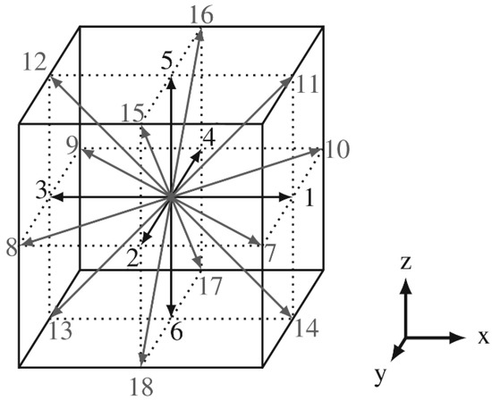
Figure 1.
Lattice velocity vectors of the D3Q19 model.
At low Mach numbers, Taylor expansion is carried out around zero particle velocity, and the Maxwell equilibrium distribution function is approximately
The macroscopic density ρ and velocity u are given by
is the weight factor associated with the ith direction which is given as
The collision matrix Ω in Equation (1) can be described by
M is a constant matrix for the D3Q19 model and is given in Ref. [38]. S is the relaxation matrix, as shown in Equation (7) [39].
The relaxation rate sυ is related to the kinematic viscosity υ as
τ is the relaxation time, which is related to the kinematic viscosity of fluid as with sound speed . The lattice speed of sound cs is a constant depending on the choice of the lattice. The lattice-spacing δx and time-step δt are defined as 1 lu and 1 ts (lu and ts refer to lattice units and time step, respectively, in the LB method). The kinematic viscosity of fluid is defined as υ = 1/6 lu2/ts, and the relaxation time is defined as τ = 1. The relationship between viscosity and relaxation time is obtained by the recovery of the Navier–Stokes equation. In the Chapman–Enskog expansion of the LB equation, the term is equivalent to the viscosity in the Navier–Stokes equation. More details about the Chapman–Enskog expansion used to recover the Navier–Stokes equation can be found in Refs. [40,41,42,43].
In an incompressible fluid, the Navier–Stokes equation is governed by the laws for mass and momentum conservation:
Here, u is the velocity, and the index p indicates that variables and derivatives are evaluated in physical units. pp is the pressure and υp the kinematic viscosity in physical units.
The Navier–Stokes equation is now cast into a dimensionless form. For this, a length scale l0 and a time scale t0 are introduced, which are representative for the flow configuration. The length l0 could, for example, stand for the size of an obstacle which is immersed in the fluid, and t0 could be the time needed by a passive scalar in the fluid to travel a distance l0. The physical variables, such as the time tp and the position vector xp, are replaced by their dimensionless counterpart: td = tp/t0 and xd = xp/l0. In the same manner, a unit conversion is introduced for other variables, based on a dimensional analysis: up = l0ud/t0, ∂tp = ∂td/t0, p = d/l0, and . Plugging this change of variables into the Navier–Stokes equation leads to the dimensionless version of the Navier–Stokes equations:
The dimensionless Reynolds number has been defined as Re = , evaluated in any system of units. Two flows obeying the Navier–Stokes equation are equivalent if they are embedded in the same geometry (except for a scaling factor) and have the same Reynolds number.
2.2. Boundary Condition
Three kinds of boundary conditions are adopted, i.e., the half-way bounce-back (BB) boundary condition, the Maxwellian diffuse (MD) reflection boundary condition, and the inlet/outlet boundary condition and the periodic boundary condition.
In the continuum flow regime, the half-way bounce-back boundary condition [44] is applied to obtain the unknown components of the distribution function at nodes neighboring solid nodes. It assumes that the no-slip solid wall is located half-way between the pore and solid nodes. The distribution functions from the fluid node streaming to their neighboring solid nodes scatter back to the fluid node along its incoming direction.
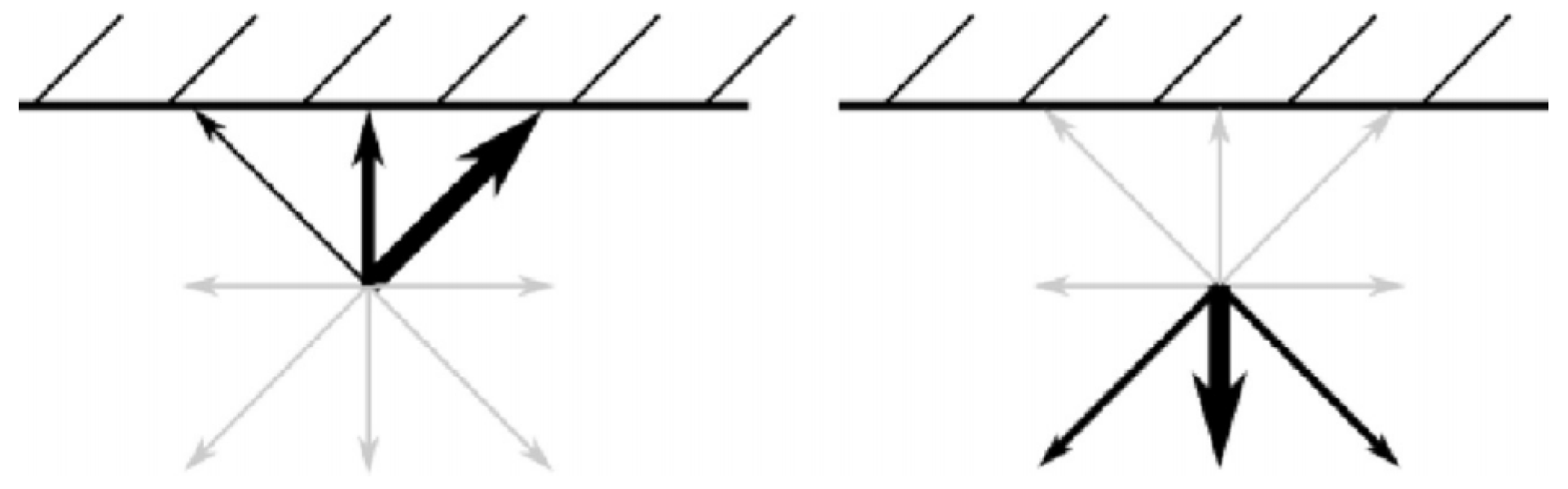
For micro-gaseous flow simulation in the transition flow regime with the high Kn effect, the Maxwellian diffuse (MD) reflection boundary condition [17,18] is adopted. The underlying idea of this boundary condition is that impinging particles lose the memory of their movement direction and are scattered back following a Maxwellian distribution in which the wall density (ρw) and the wall velocity (uw) are known. A general form of diffusive boundary, which is applicable for both channel and porous media, is expressed as , where i is the direction in which the distribution function is unknown; j is the direction pointing to solid cell. The process of the boundary treatment is illustrated in Figure 2. Consistent with the microscopic collision behavior of gas molecules at solid surfaces, the MD reflection boundary condition more accurately simulates real-world boundary interactions, especially for rough or irregular surfaces, and handles boundary slip more naturally. Easier to implement, the MD reflection boundary condition simplifies handing of complex geometries.

Figure 2.
Illustration of the diffuse process. (In the left image, the distributions before the collision and in the right image, the diffusive distributions collided with the wall are shown. The thickness of the arrows indicates the value of the distributions.)
The pressure boundary conditions at the inlet and outlet are firstly dealt with using the moment-based boundary conditions [45]. Taking the D3Q19 model as an example, if the inlet and outlet boundary faces are perpendicular to the z-direction (as in Figure 1) and the density at the inlet and outlet is set as a constant, then, after the streaming step, the components of the distribution function at the inlet boundary (i.e., f5, f11, f12, f15, and f16) or outlet boundary (i.e., f6, f13, f14, f17, and f18) are unknown. The unknown components at the inlet/outlet boundary satisfy the following equations:
At the inlet boundary (i.e., bottom boundary):
At the outlet boundary (i.e., top boundary):
With the periodic boundary condition, the components of the particle distribution functions exiting from one boundary will directly enter into the opposite boundary:
2.3. Unit Conversion
For the application of the LBM simulation, it is necessary to establish the conversion relationship between lattice units and real physical units [40]. For the basic physical quantities (length, time, and mass), the conversion relationship between lattice units (x, t, ρ) and real physical units (xp, tp, ρp) is xL0→xp, tT0→tp, ρM0→ρp, which is sufficient to generate the dimension of any mechanical quantity. For example, the fluid domain (100 × 100 × 100 μm3 in the physical system) is digitized into 200 × 200 × 200 lattices. Thus, L0 = 5 × 10⁻⁷ m, since a lattice spacing δx = 1. The density of water is given as ρp = 1000 kg/m3, and the density is set to ρ = 1 in the LBM simulation. Since density has dimensions [M][L]−3, ρp = M0 L0−3 ρ; hence, M0 = 1.25 × 10⁻¹⁶ kg.
2.4. Permeability Calculation
In the LBM simulation, a pressure (density) difference is applied at the inlet and outlet sides to drive the flow in porous media. The other four sides are considered periodic boundaries. The convergence criterion for attaining the steady-state solution is decided every 10 iteration steps, which is defined as
where i, j, and k are the lattice nodes in the x-, y-, and z-directions, respectively. The threshold value of 1.0 × 10⁻⁵ is found not only to be sufficient to guarantee the computational accuracy, but is also helpful to reduce the computing time and memory requirements.
Reaching the convergence criteria for attaining the steady-state solution, the permeability in LB units can be calculated according to Darcy’s law [46]:
denotes the overall mean value of velocity in the z-direction, is the pressure gradient, and Nx, Ny, and Nz are the numbers of discretization nodes in the x, y and z-direction, respectively. ρin and ρout denote the density at the inlet and outlet, respectively.
The permeability K in physical units can be obtained from that in lattice units:
3. Validation of the MRT-LBM
To verify the reliability and accuracy of the MRT-LBM, two benchmark tests, that is, 3D Poiseuille flow and flow through a body-centered cubic array of spheres, are employed here. To validate the performance for rarefied gas flows using the MRT-LBM combined with a Bosanquet-type effective viscosity model and the Maxwellian diffuse reflection boundary condition, the micro-channel flow at high Kn numbers is also simulated as a benchmark.
3.1. Poiseuille Flow in a 3D Square Channel
For the 3D Poiseuille flow driven by a pressure gradient in a channel with a cross-section size H × H, the analytical solution of the X-component velocity is
where Y ∈ [H/2, H/2] and Z ∈ [H/2, H/2] are the coordinates in the cross-section with the center of the channel as origin, and L is the length of the channel. Pout and Pin are the pressures at the outlet and inlet boundary, respectively.
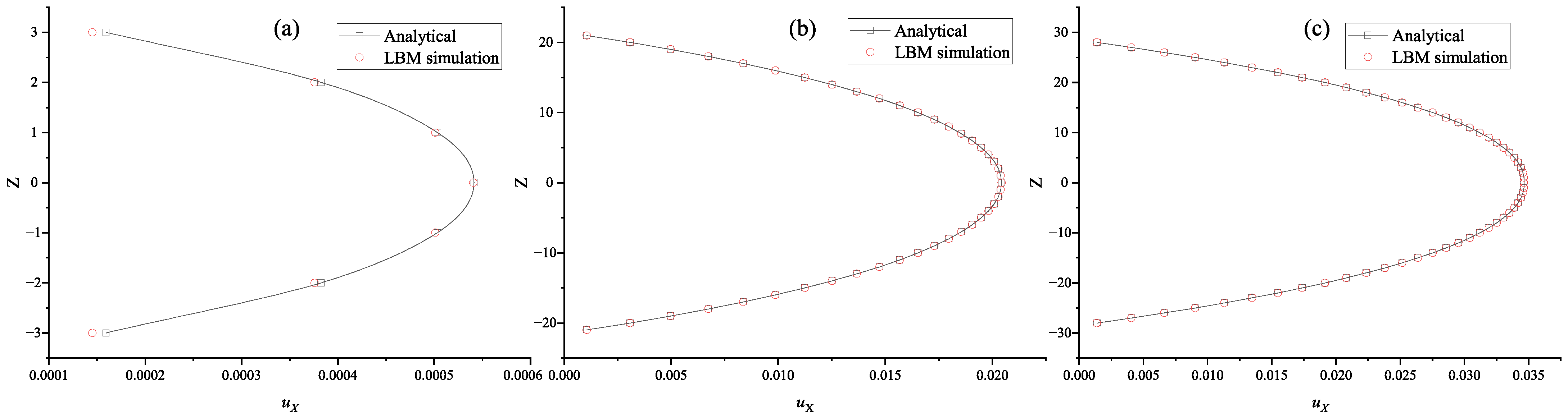
To choose a grid size yielding trustworthy results and utilizing less computational resources, the grid independence test is performed under different grid resolutions (e.g., coarse, medium, and fine resolution). The L2 error of the analytical solution is, respectively, 3.430861 × 10⁻², 8.453364 × 10⁻⁴, and 5.785233 × 10⁻⁴, where the L2 error is measured by . As shown in Figure 3, the grid size of 86 × 43 × 43 of the computational domain is adequate for obtaining a trustworthy solution. Using the grid size of 86 × 43 × 43, the contour of the X-component velocity uX in the Poiseuille flow is present in Figure 4, which shows that the numerical results are in good agreement with the analytical solution.
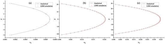
Figure 3.
Distribution of the X-component velocity uX on the line of X = 0.5 L, Y = 0 in the Poiseuille flow under different grid resolutions: (a) 13 × 7 × 7, (b) 86 × 43 × 43 (c) 104 × 56 × 56.
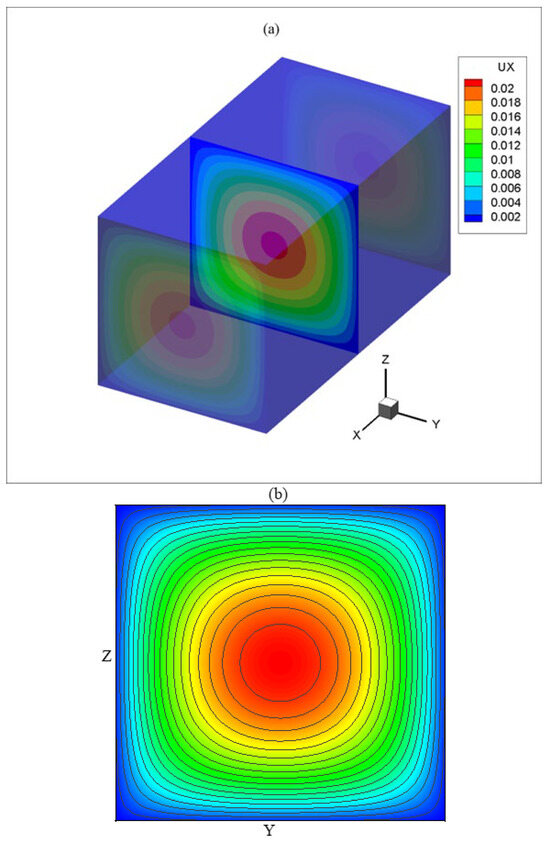
Figure 4.
Distribution of the X-component velocity uX in the Poiseuille flow: (a) the 3D contour, (b) the slice of X = 0.5 L.
3.2. Flow Through a Body-Centered Cubic Array of Spheres
An open cube filled with a periodic body-centered cubic (BCC) array of spheres is depicted in Figure 5. A grid of 50 × 50 × 50 is used. The non-slip solid wall adopts half of the back-bound rule, the inlet and outlet adopt the moment-based boundary condition [45] (as shown in Equations (9) and (10)), and the other four walls adopt the periodic boundary condition (as shown in Equation (11)).
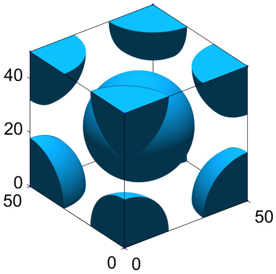
Figure 5.
A periodic body-centered cubic array of spheres (blue and white areas represent solid and pore regions, respectively).
The analytical intrinsic permeability k for BCC arrays of spheres is calculated by
G is a coefficient that is equal to 12 for BCC. R and L represent the radius of the solid spheres and length of cubic samples, respectively; Cd is the drag coefficient and was presented in Ref. [47].
The value of k can be transformed to a dimensionless permeability [48]:
Figure 6 shows the velocity distribution of fluid under steady-state conditions (Equation (12)) in the samples (Figure 5) using the boundary conditions in Section 2.2. For the treatment of the pressure boundary condition at the inlet and outlet, the non-equilibrium bounce-back (NEBB) boundary condition [49] is used for comparison with the moment-based boundary condition. The comparisons between the results obtained by the NEBB and moment-based boundary condition are shown in Table 1. The simulated results are in good agreement with the analytical solutions with different porosities. With the low-resolution grid of 50 × 50 × 50, the error is only less than 4 percent. It is noted that Δ1 represents the percentage error of the moment-based boundary relative to the analytical solution, and Δ2 represents the percentage error of the NEBB boundary relative to the analytical solution.
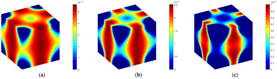
Figure 6.
Velocity (U = sqrt(ux2 + uy2 + uz2)) distribution of fluid through BCC arrays of spheres. (a) R = 11, (b) R = 15, (c) R = 19.

Table 1.
Dimensionless permeability k* obtained by the LBM simulation with the NEBB and moment-based boundary condition.
3.3. Mircochannel Flow at High Kn Number
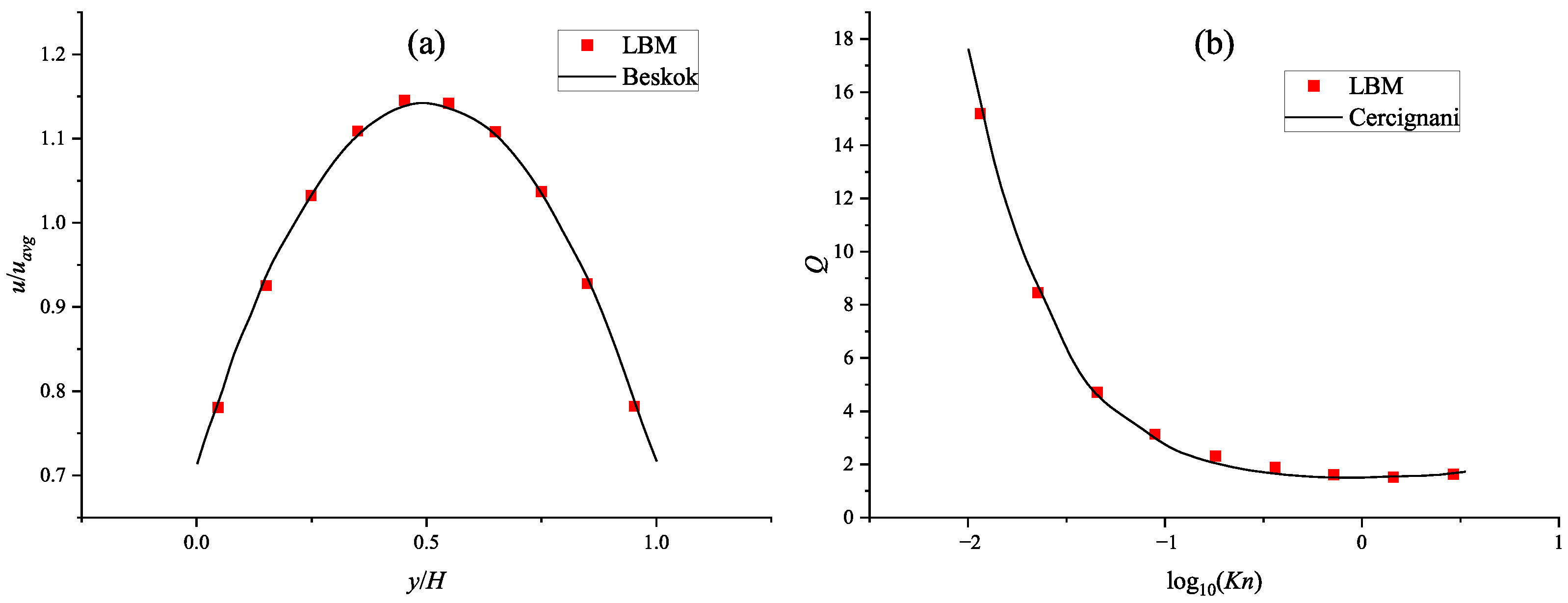
To validate the performance for rarefied gas flows, the micro-channel flow at high Kn numbers is simulated as a benchmark, using the MRT-LBM combined with the Bosanquet-type effective viscosity model and Maxwellian diffuse reflection boundary condition. The fluid is treated as an ideal gas. The temperature is T = 373 K, molar mass is M = 0.016 kg/mol, pressure gradient p = −1 MPa/m, channel height is H = 10 nm, and dynamic viscosity is μ = 10−5 kg/m/s. The Knudsen (Kn) number is defined as Kn = λ/l. λ is the mean free path of the gas molecules, where μ is the dynamic viscosity of gas; ρ is the gas density; M is the molar mass; T is the absolute temperature; and R is the gas constant. l is the characteristic length. Under these conditions, the Kn number is obtained (Kn = 0.712). The gas viscosity is described by the Bosanquet-type effective viscosity model, μe = μ/(1 + aKn), with the empirical parameter a = 2.2, as suggested by Beskok and Karniadakis [50]. Figure 7a compares the cross-section velocity profile obtained by the present MRT-LBM simulation with Beskok’s model [50]. The fluid density ρ is doubled from 1 kg/m3 to 256 kg/m3 successively. Figure 7b compares the normalized mass flow rate in the present work with Cercignani’s theoretical solution [51]. The agreement between the present numerical simulations and the theoretical models is very good. Thus, the present method for high Kn flow is reliable for further exploration.
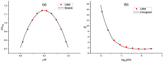
Figure 7.
Comparison of LBM simulation and theoretical modeling of high Kn flow in channel: (a) velocity profile in the cross-section of the channel at Kn = 0.712, (b) normalized mass flow rate versus Kn.
4. Flow in Porous Media
4.1. Porous Structure Reconstruction
To study the influence of anisotropy on flow in porous media, the process of reconstructing 3D porous media by the Quarter Structure Generation Set (QSGS) method can be divided into three steps, to validate the model’s performance for rarefied gas flows at high Kn numbers:
(a) When the structural region and randomly distributed solid-phase growth nuclei (Cs) are set, the probability (Pcd) of Cs should not be greater than the porosity (ϕ) of the final three-dimensional porous media, that is, Pcd ≤ ϕ. Random numbers within [0, 1] are generated by a random number generator, and nodes with random numbers less than Pcd are designated as solid-phase growth nuclei.
(b) Given the growth rate (Pk, where k represents the growth direction of the solid phase) in different directions, random numbers within [0, 1] are generated by a random number generator. When the random number of the Cs node is less than Pk, it grows along the adjacent point in the k direction. The total number of the growth direction is set to be 26, which can be divided into the side line direction (6), diagonal line direction (12), and diameter line direction (8). When the growth rate in all directions is the same, isotropic porous media can be obtained. When the growth rates in all directions are different, anisotropic porous media can be obtained.
(c) Step (b) is repeated until the desired porosity of the porous medium is achieved.
The heterogeneity cannot be accomplished by the original QSGS algorithm. To study the influence of heterogeneity on flow in porous media, two independent generation processes can be used [27]: (i) The fine structure produces a smaller solid phase, and the nucleus growth probability of solid phase growth is Pr and the porosity is ϕR. (ii) The coarse structure produces a larger solid phase, and the nucleus growth probability of the solid phase is Pc (Pc << Pr). When the two processes are combined, the nodes occupied by either process are set as the solid phase until the desired porosity is reached. The final structure is the combination of the fine structure and coarse structure.
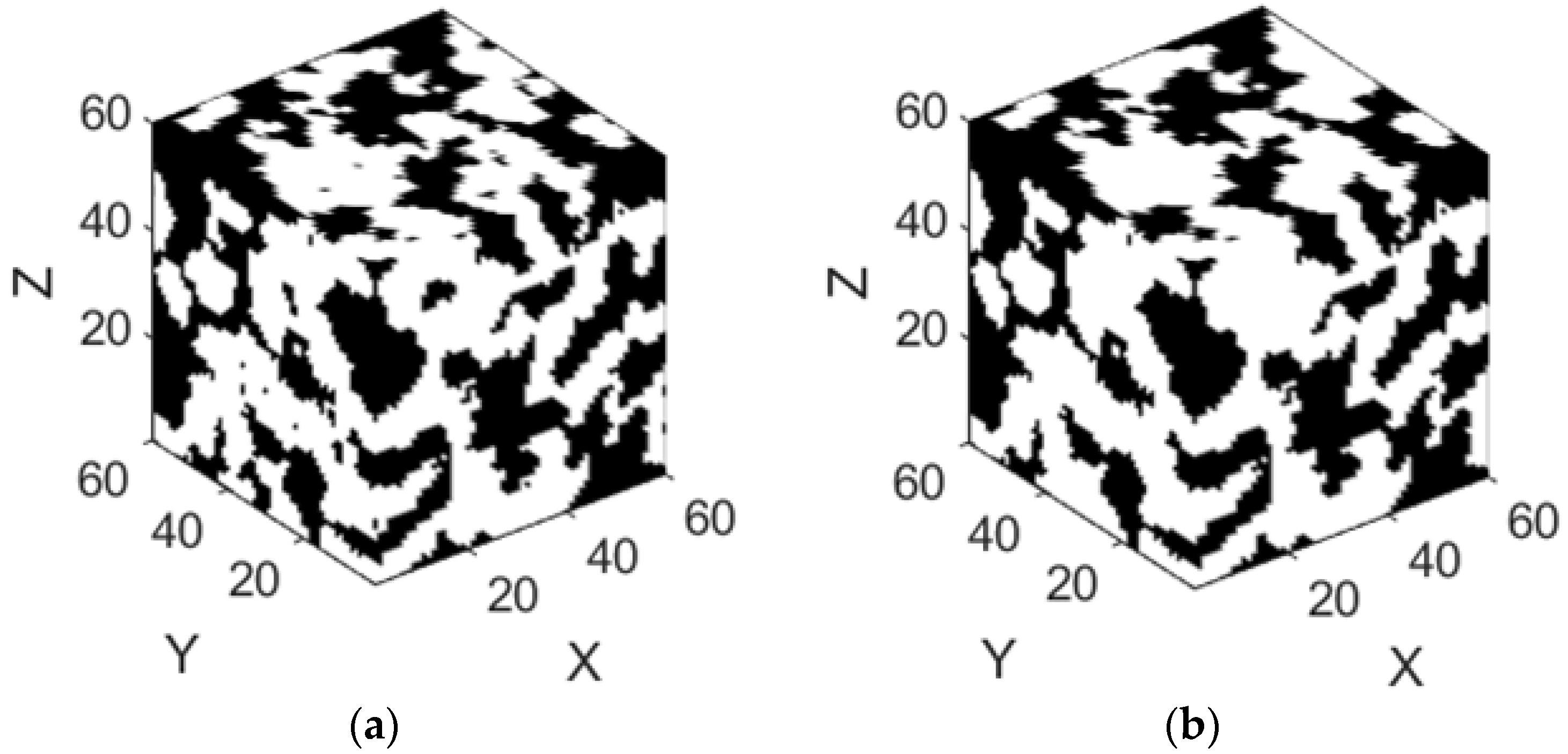
The original QSGS method can generate occluded pores, which are not connected to the main void space and do not contribute to flow. Only inter-connected pore spaces are channels for fluid flow and transport. The occluded pores in 3D porous media can be removed by improving the 4-connected component labeling (4-CCL) algorithm [52]: (a) Classify the pixels of the 3D porous media into two types: pore pixel and solid pixel. (b) Label each pore pixel with a temporary number by checking its east, west, south, north, upper, and lower neighborhoods. If none of the neighbors is labeled, a new label for the pixel is set, which increases from 1 without repeating. If only one neighbor is labeled, the pore pixel is set to the same number of marks; if two or more neighbors are labeled, the pore pixel is set to be the minimum of its neighbors’ label values. (c) Replace each temporary label by the smallest label of its equivalence class. (d) Set the occluded pores as solids and retain the pore space that connects the inlets and outlets, then update the volume fraction or the porosity. For example, the 3D views of porous media before and after removing occluded pores are shown in Figure 8.

Figure 8.
Three-dimensional view of porous media (a) before and (b) after removing occluded pores. The black represents pores and the white represents solid matrix.
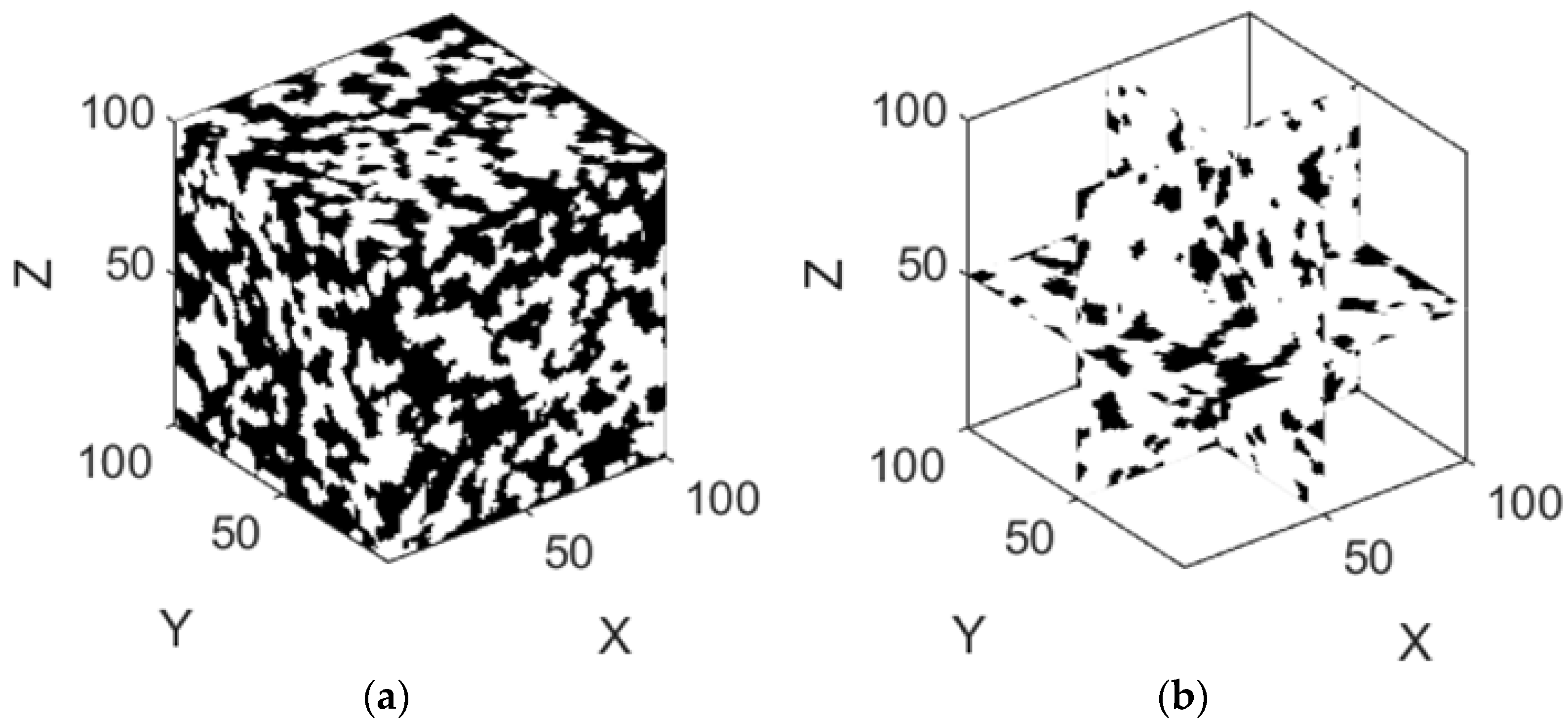
For the flow along the X direction, the solid growth rate in the Z direction is adjusted, and the 3D anisotropic porous media is established. The coarse structure and fine structure are combined to establish 3D heterogeneous porous media. The specific generation parameters are shown in Table 2. Considering the influence of random generation, 10 structures of random porous media are constructed under the same generation parameters. Figure 9, Figure 10, Figure 11 and Figure 12 show one group of anisotropic porous media.
Table 2.
The parameters for the reconstructed structure of pore media in simulation.
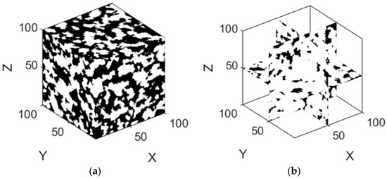
Figure 9.
Three-dimensional view of one group of the reconstructed anisotropic structures, with pores represented by black and solid matrix by white. The growth rate ratio is 1. (a) 3D global diagram, (b) 3D slice diagram.
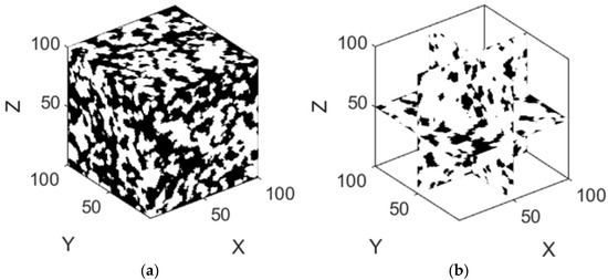
Figure 10.
Three-dimensional view of one group of the reconstructed anisotropic structures, with pores represented by black and solid matrix by white. The growth rate ratio is 2. (a) 3D global diagram, (b) 3D slice diagram.

Figure 11.
Three-dimensional view of one group of the reconstructed anisotropic structures, with pores represented by black and solid matrix by white. The growth rate ratio is 4. (a) 3D global diagram, (b) 3D slice diagram.
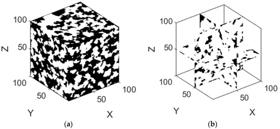
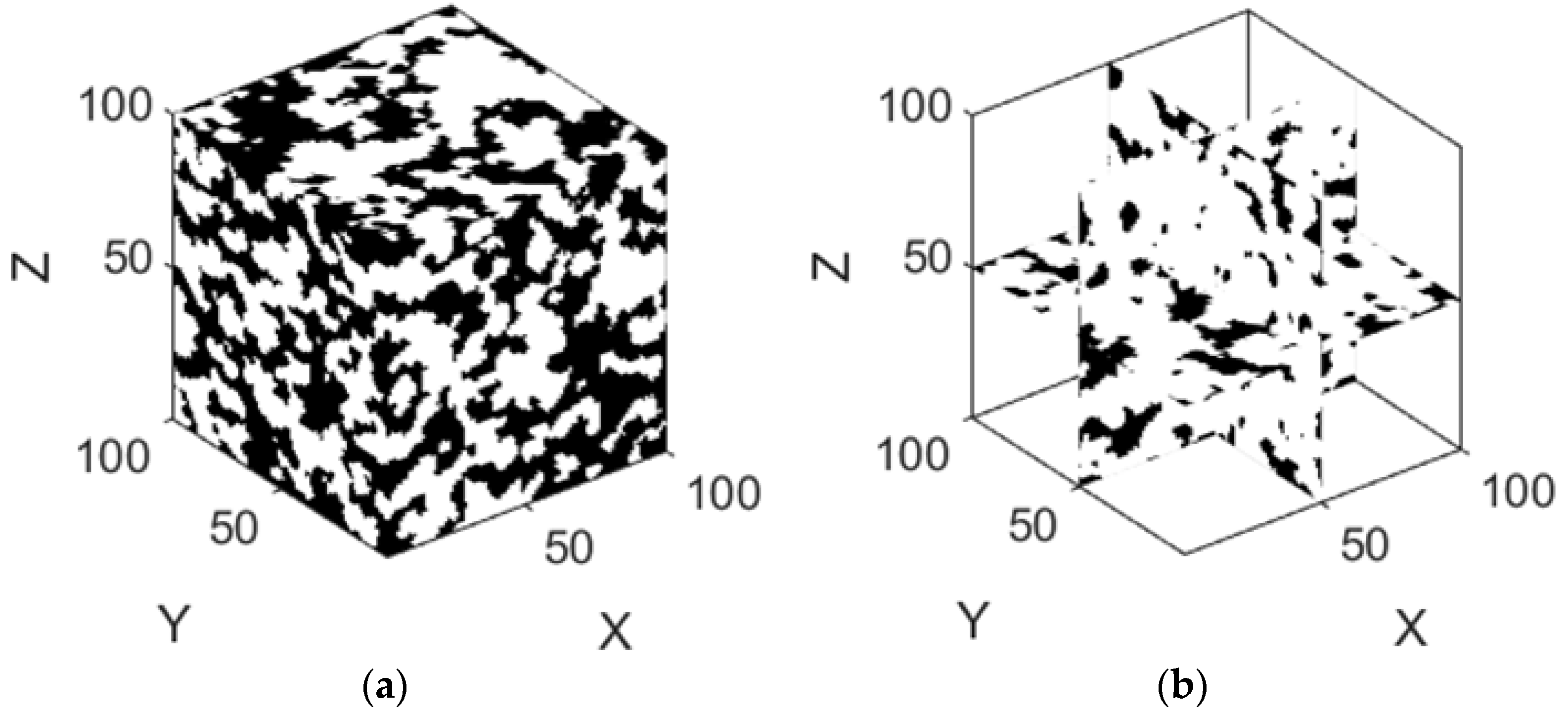
Figure 12.
Three-dimensional view of one group of the reconstructed anisotropic structures, with pores represented by black and solid matrix by white. The growth rate ratio is 8. (a) 3D global diagram, (b) 3D slice diagram.
4.2. Effect of Anisotropy and Heterogeneity
The anisotropy model and heterogeneity model proposed by Wang et al. [27] are used to quantitatively evaluate the pore-scale anisotropy factor (A) and heterogeneity (H). we consider a line crossing the structure along the x direction and define the average pore number it can encounter per unit length as nx. Similarly, we can define ny in the y direction. The anisotropy of the pore structure is defined as A = nx/ny. We firstly define the observation scale lx, ly, and lz along the x, y, and z direction, respectively. After that, we divide the whole porous structure into blocks with side lengths of lx, ly, and lz. Then we use the relative standard deviation of each block’s porosity to quantify the heterogeneity of pore distribution: , where Φi is the porosity of the ith block and f is the total porosity.
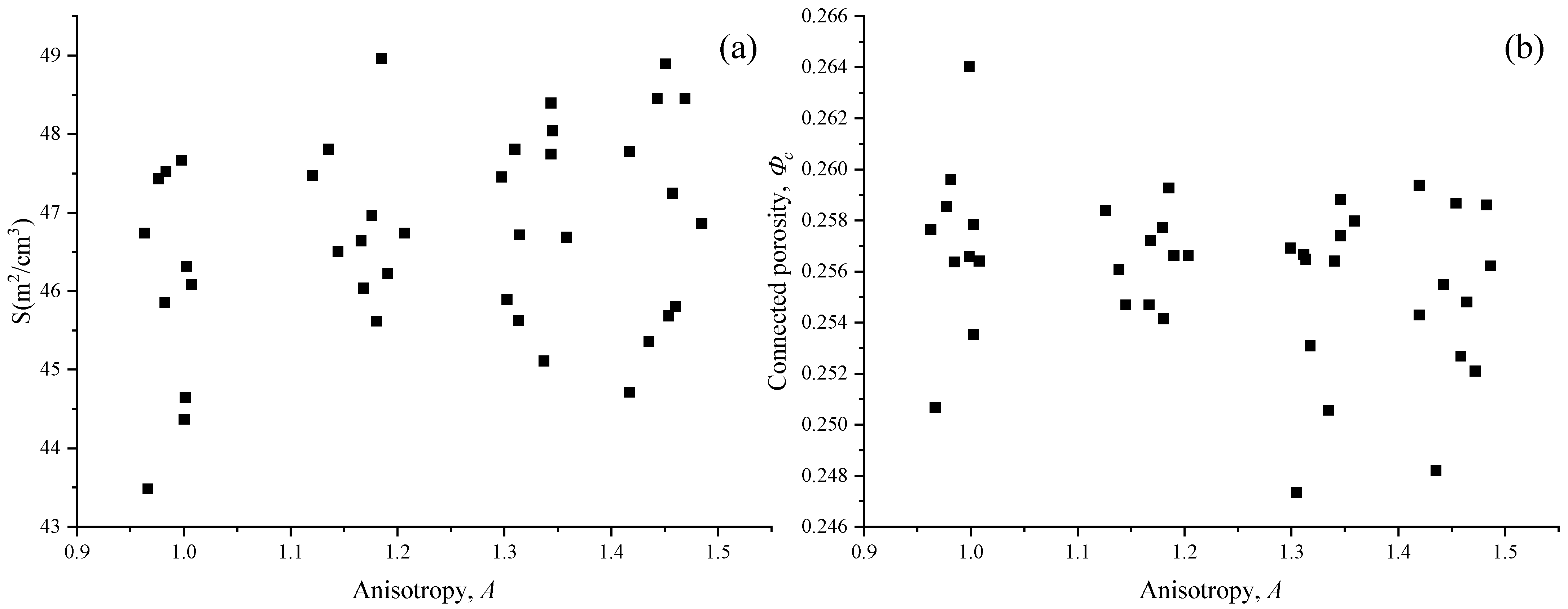
The relationship between connected porosity (Φc), the ratio of surface area to volume (S), and the pore-scale anisotropy factor (A) of the generated porous media is shown in Figure 13. It can be seen that with the increase in the anisotropy factor (A), the change percentage of value Φc and S is less than 2%. The relationship between the connected porosity (Φc), the ratio of surface area to volume (S), and the heterogeneity factor H of the generated porous medium is shown in Figure 14. It can be seen that the connected porosity of porous media is weakly affected by heterogeneity, and the change percentage is less than 4%. The ratio S has an obvious negative correlation with the heterogeneity factor, and S decreases by about 21% with the increase in the heterogeneity factor.
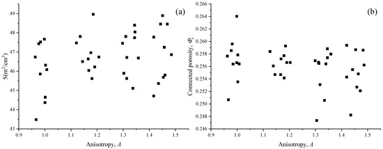
Figure 13.
(a) S vs. A, (b) Φc vs. A.
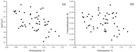
Figure 14.
(a) S vs. H, (b) Φc vs. H.
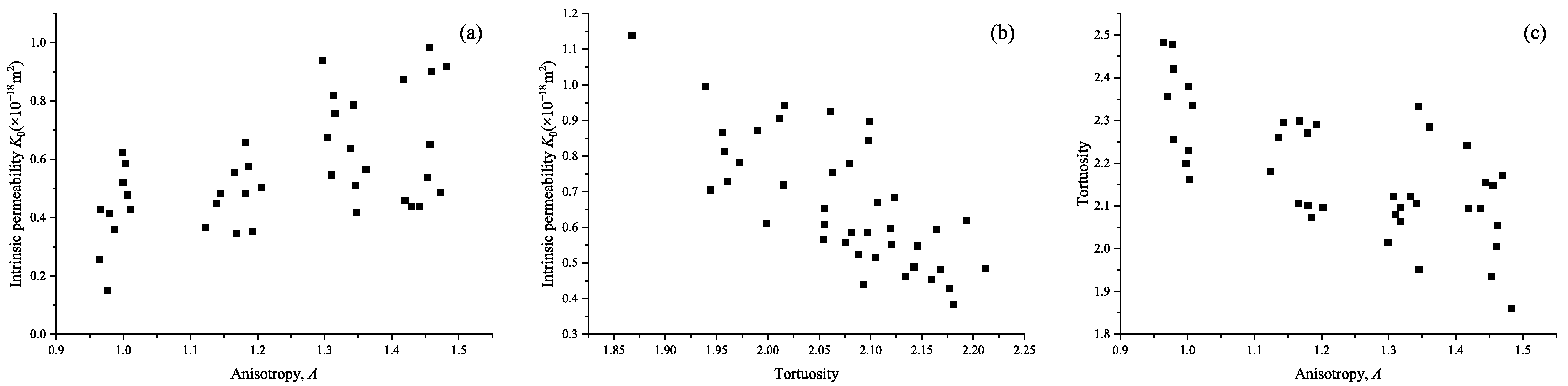
We firstly simulate the steady-state non-slip flow by the LBM to determine the intrinsic permeability. The boundary condition of the non-slip wall is treated by the half-way bounce-back rule to simulate gas flow in a continuum flow regime, and the intrinsic permeability (K0) and tortuosity (τ) are obtained. The relationship between the calculated intrinsic permeability, tortuosity, and anisotropy factor is shown in Figure 15. The intrinsic permeability of anisotropic porous media is positively correlated with the anisotropy factor. Intrinsic permeability is negatively correlated with tortuosity. Tortuosity is negatively correlated with the anisotropy factor. The relationship among intrinsic permeability, the heterogeneity factor, the ratio of surface area to volume, and tortuosity is shown in Figure 16. It can be seen that the intrinsic permeability is positively correlated with the heterogeneity factor, and the intrinsic permeability increases by about 136% with the increase in the heterogeneity factor. There is no obvious correlation between intrinsic permeability and the ratio of surface area to volume. There is an obvious negative correlation between intrinsic permeability and tortuosity. There is no obvious correlation between tortuosity and the heterogeneity factor.
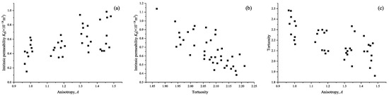
Figure 15.
(a) K0 vs. A, (b) K0 vs. τ, (c) τ vs. A.
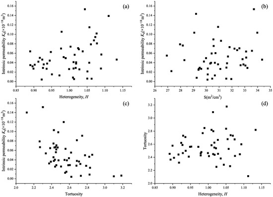
Figure 16.
(a) K0 vs. H, (b) K0 vs. S, (c) K0 vs. τ, (d) τ vs. H.
The pore-scale anisotropy significantly affects the tortuosity, and the heterogeneity of pore distribution significantly affects the ratio of surface area to volume, and then significantly affects the flow in porous media. (1) The larger the anisotropy factor in the mainstream direction, the stronger the orientation of the long axis of pores along the mainstream direction, and the flatter the flow path. The tortuosity is significantly reduced, the energy consumed by fluid flowing through porous media is reduced, and the permeability of porous media is enhanced. The strong correlation between tortuosity and anisotropy is the fundamental reason why anisotropy affects permeability. (2) The larger the size of solid particles in porous media, the more obvious the phenomenon of pore aggregation, the higher the probability of overlapping between pores, and the ratio of surface area to volume is significantly reduced. When the porosity of porous media is almost identical, the larger the solid particles or the smaller the ratio of surface area to volume, the smaller the wall friction resistance of fluid flowing through porous media, and the greater the permeability of porous media. (3) Although there is no obvious correlation between permeability and the ratio of surface area to volume of 3D heterogeneous porous media, the general trend is that permeability increases with the increase in heterogeneity factor. This is because tortuosity is also an important factor affecting the permeability of porous media. Tortuosity is related to the arrangement direction and position of solid particles (especially the large solid particles) in porous media. In the 3D heterogeneous porous media, with the enhancement of heterogeneity, the difference between solid particles increases, and the randomness of distribution position may lead to a random change in tortuosity, which may increase or decrease, resulting in no obvious correlation between tortuosity and heterogeneity. The permeability of porous media is affected by heterogeneity of pore distribution due to the combined action of tortuosity and the ratio of surface area to volume.
4.3. Effect of Slip
Then, the apparent permeability K at a certain Kn number is predicted by introducing the Maxwellian diffuse (MD) reflection boundary condition [17,18] and Bosanquet-type effective viscosity model [25] in the LBM. With the apparent permeability K at a certain Kn number, the slip factor b reflecting the micro-scale slip effect is calculated by
For porous media, the Knudsen (Kn) number is defined: Kn = λ/l. λ is the mean free path of the gas molecules, where μ is the dynamic viscosity of gas; ρ is the gas density; M is the molar mass; T is the absolute temperature; and R is the gas constant. L = 2Vp/Sin is the characteristic length. Vp is the pore volume and Sin is the interface area between the pore and solid. K is the apparent permeability and K0 is the intrinsic permeability, both obtained through the LBM simulation.
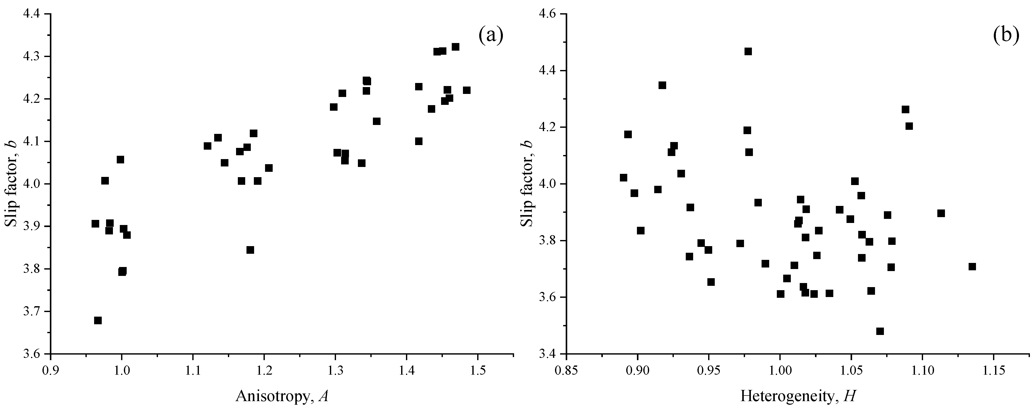
As shown in Figure 17a, the slip factor (b) is positively correlated with the anisotropic factor (A), and b increases with the increase in A, which means that the high Kn effect is stronger in anisotropic structures. When gas passes through anisotropic porous media, it more easily interacts with the wall, and the confinement effect is more significant. As shown in Figure 17b, there is no obvious correlation between the slip factor and structural heterogeneity of the structure. The heterogeneity does not influence the pore geometry. As shown in Figure 16d, with the enhancement of heterogeneity, the randomness of the distribution position may lead to a random change in tortuosity, which may increase or decrease.
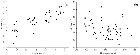
Figure 17.
(a) b vs. A, (b) b vs. H.
5. Conclusions
The Quartet Structure Generation Set (QSGS) method is improved to construct anisotropic and heterogeneous three-dimensional porous media, which cannot generate occluded pores. Using the MRT-LBM, the pressure boundary conditions at the inlet and outlet are firstly dealt with using the moment-based boundary conditions, demonstrating good agreement with the analytical solutions in two benchmark tests of 3D Poiseuille flow and flow through a body-centered cubic array of spheres. Combined with the Bosanquet-type effective viscosity model and Maxwellian diffuse reflection boundary conditions, the performance of the MRT-LBM for rarefied gas flows at high Kn numbers is validated. Then, the gas flow at high Kn values in three-dimensional porous media is simulated to study the relationship between pore-scale anisotropy, heterogeneity, and Kn, and permeability and micro-scale slip effects in porous media. The following findings are obtained:
- (1)
- The intrinsic permeability of anisotropic porous media is positively correlated with anisotropy factor and negatively correlated with tortuosity. Tortuosity is negatively correlated with anisotropy factor. The intrinsic permeability of heterogeneous porous media is positively correlated with the heterogeneity factor of pore distribution, but has no obvious correlation with the ratio of surface area to volume, and has an obvious negative correlation with tortuosity. There is no obvious correlation between tortuosity and the heterogeneity factor.
- (2)
- The pore-scale anisotropy significantly affects the tortuosity of porous media, and the heterogeneity of pore distribution significantly affects the specific surface area, and then significantly affects the flow in porous media. The strong correlation between tortuosity and anisotropy is the fundamental reason why anisotropy affects permeability. With the increase in heterogeneity of pore distribution, the ratio of surface area to volume decreases significantly, the wall friction resistance of fluid flowing through porous media decreases, and the permeability of porous media increases.
- (3)
- The slip factor is positively correlated with the anisotropic factor, which means that the high Kn effect is stronger in anisotropic structures. There is no obvious correlation between the slip factor and heterogeneity factor. With the enhancement of heterogeneity, the randomness of the distribution position may lead to the random change in tortuosity.
This study may be very helpful for a better understanding of the gas transport mechanism in porous heat shields for the aerospace industry and for possible process optimization of transpiration cooling. This study does not consider the condition in which the gas is under high pressure and high temperature so that the real gas (or non-ideal gas) effect is significant. So, the real gas effect will be studied in the gas transport mechanism in porous media in future.
Author Contributions
Conceptualization, W.G.; methodology, W.G., J.Z. and G.W.; software, W.G.; validation, W.G., J.Z. and G.W.; formal analysis, W.G.; investigation, W.G.; resources, W.G., J.Z., G.W., M.F. and K.Z.; data curation, W.G.; writing—original draft preparation, W.G.; writing—review and editing, W.G., J.Z., G.W., M.F. and K.Z.; visualization, W.G.; supervision, M.F.; project administration, M.F.; funding acquisition, M.F. All authors have read and agreed to the published version of the manuscript.
Funding
This research received no external funding.
Data Availability Statement
The data that supports the findings of this study are available within the article.
Conflicts of Interest
The authors declare no conflict of interest.
References
- Poovathingal, S.; Stern, E.C.; Nompelis, I.; Schwartzentruber, T.E.; Candler, G.V. Nonequilibrium flow through porous thermal protection materials, Part II: Oxidation and pyrolysis. J. Comput. Phys. 2019, 380, 427–441. [Google Scholar] [CrossRef]
- Van Foreest, A.; Sippel, M.; Gülhan, A.; Esser, B.; Ambrosius, B.A.; Sudmeijer, K.J. Transpiration cooling using liquid water. J. Thermophys. Heat Transf. 2009, 23, 693–702. [Google Scholar] [CrossRef]
- Glass, D. Ceramic matrix composite (CMC) thermal protection systems (TPS) and hot structures for hypersonic vehicles. In Proceedings of the 15th AIAA International Space Planes and Hypersonic Systems and Technologies Conference, Dayton, OH, USA, 28 April–1 May 2008; American Institute of Aeronautics and Astronautics: Dayton, OH, USA, 2008; p. 2682. [Google Scholar]
- Khabbazi, A.E.; Hinebaugh, J.; Bazylak, A. Determining the impact of rectangular grain aspect ratio on tortuosity-porosity correlations of two-dimensional stochastically generated porous media. Sci. Bull. 2016, 61, 601–611. [Google Scholar] [CrossRef]
- Wang, J.; Li, C.; Kang, Q.; Rahman, S.S. The lattice Boltzmann method for isothermal micro-gaseous flow and its application in shale gas flow: A review. Int. J. Heat Mass Transf. 2016, 95, 94–108. [Google Scholar] [CrossRef]
- Ranjbarzadeh, R.; Sappa, G. Numerical and experimental study of fluid flow and heat transfer in porous media: A review article. Energies 2025, 18, 976. [Google Scholar] [CrossRef]
- D’Orazio, A.; Karimipour, A.; Ranjbarzadeh, R. Lattice Boltzmann modelling of fluid flow through porous media: A comparison between pore-structure and representative elementary volume methods. Energies 2023, 16, 5354. [Google Scholar] [CrossRef]
- Zahid, F.; Cunningham, J.A. Review of the Color Gradient Lattice Boltzmann Method for Simulating Multi-Phase Flow in Porous Media: Viscosity, Gradient Calculation, and Fluid Acceleration. Fluids 2025, 10, 128. [Google Scholar] [CrossRef]
- Ho, M.; Tucny, J.-M.; Ammar, S.; Leclaire, S.; Reggio, M.; Trépanier, J.-Y. Lattice Boltzmann Model for Rarefied Gaseous Mixture Flows in Three-Dimensional Porous Media Including Knudsen Diffusion. Fluids 2024, 9, 237. [Google Scholar] [CrossRef]
- Atykhan, M.; Dauyeshova, B.K.; Monaco, E.; Rojas-Solórzano, L.R. Modeling Immiscible Fluid Displacement in a Porous Medium Using Lattice Boltzmann Method. Fluids 2021, 6, 89. [Google Scholar] [CrossRef]
- Lei, G.; Liu, T.; Liao, Q.; He, X. Estimating permeability of porous media from 2D digital images. J. Mar. Sci. Eng. 2023, 11, 1614. [Google Scholar] [CrossRef]
- Farahani, M.V.; Nezhad, M.M. On the effect of flow regime and pore structure on the flow signatures in porous media. Phys. Fluids 2022, 34, 115139. [Google Scholar] [CrossRef]
- Farahani, M.V.; Foroughi, S.; Norouzi, S.; Jamshidi, S. Mechanistic study of fines migration in porous media using lattice Boltzmann method coupled with rigid body physics engine. J. Energy Resour. Technol. 2019, 141, 123001. [Google Scholar] [CrossRef]
- Chalmers, G.R.; Bustin, R.M.; Power, I.M. Characterization of gas shale pore systems by porosimetry, pycnometry, surface area, and field emission scanning electron microscopy/transmission electron microscopy image analyses: Examples from the Barnett, Woodford, Haynesville, Marcellus, and Doig units. AAPG Bull. 2012, 96, 1099–1119. [Google Scholar]
- Succi, S. The Lattice-Boltzmann Equation; Oxford University Press: Oxford, UK, 2001. [Google Scholar]
- Tao, S.; Guo, Z. Boundary condition for lattice Boltzmann modeling of microscale gas flows with curved walls in the slip regime. Phys. Rev. E 2015, 91, 043305. [Google Scholar] [CrossRef] [PubMed]
- Ansumali, S.; Karlin, I.V. Kinetic boundary conditions in the lattice Boltzmann method. Phys. Rev. E 2002, 66, 026311. [Google Scholar] [CrossRef]
- Zhao, J.; Yao, J.; Li, A.; Zhang, M.; Zhang, L.; Yang, Y.; Sun, H. Simulation of microscale gas flow in heterogeneous porous media based on the lattice Boltzmann method. J. Appl. Phys. 2016, 120, 579. [Google Scholar] [CrossRef]
- Guo, Z.; Zheng, C. Analysis of Lattice Boltzmann Equation for Microscale Gas Flows: Relaxation Times, Boundary Conditions and the Knudsen Layer; Taylor & Francis, Inc.: Abingdon, UK, 2008. [Google Scholar]
- Succi, S. Mesoscopic modeling of slip motion at fluid-solid interfaces with heterogeneous catalysis. Phys. Rev. Lett. 2002, 89, 064502. [Google Scholar] [CrossRef]
- Verhaeghe, F.; Luo, L.; Blanpain, B. Lattice Boltzmann modeling of microchannel flow in slip flow regime. J. Comput. Phys. 2009, 228, 147–157. [Google Scholar] [CrossRef]
- Eu, B.C.; Khayat, R.E.; Billing, G.D.; Nyeland, C. Nonlinear transport coefficients and plane Couette flow of a viscous, heat-conducting gas between two plates at different temperatures. Can. J. Phys. 1987, 65, 1090–1103. [Google Scholar] [CrossRef]
- Myong, R. A generalized hydrodynamic computational model for rarefied and microscale diatomic gas flows. J. Comput. Phys. 2004, 195, 655–676. [Google Scholar] [CrossRef]
- Wang, L.; Wang, S.H.; Zhang, R.L.; Wang, C.; Xiong, Y.; Zheng, X.; Li, S.; Jin, K.; Rui, Z. Review of multi-scale and multi-physical simulation technologies for shale and tight gas reservoirs. J. Nat. Gas. Sci. Eng. 2017, 37, 560–578. [Google Scholar] [CrossRef]
- Michalis, V.K.; Kalarakis, A.N.; Skouras, E.D.; Burganos, V.N. Rarefaction effects on gas viscosity in the Knudsen transition regime. Microfluid. Nanofluidics 2010, 9, 847–853. [Google Scholar] [CrossRef]
- Li, Q.; He, Y.L.; Tang, G.H.; Tao, W.-Q. Lattice Boltzmann modeling of microchannel flows in the transition flow regime. Microfluid. Nanofluidics 2011, 10, 607–618. [Google Scholar] [CrossRef]
- Wang, Z.Y.; Jin, X.; Wang, X.Q.; Sun, L.; Wang, M. Pore-scale geometry effects on gas permeability in shale. J. Nat. Gas. Sci. Eng. 2016, 34, 948–957. [Google Scholar] [CrossRef]
- Zheng, Q.; Yu, B.M.; Duan, Y.G.; Fang, Q. A fractal model for gas slippage factor in porous media in slip flow regime. Chem. Eng. Sci. 2013, 87, 209–215. [Google Scholar] [CrossRef]
- Ren, X.; Li, A.; Wang, Y.; Jiang, K.; Chen, M. Gas Permeability Experimental Study of Low Permeability Core Considering Effect of Gas Slippage. Nat. Gas. Geosci. 2015, 26, 733–736. [Google Scholar]
- Zhu, Y.; Tao, G.; Fang, W.; Wang, S. Research progress of the Klinkenberg Effect in Tight Gas Reservoir. Progress. Geophys. 2007, 22, 1591–1596. [Google Scholar]
- Duan, Q.; Yang, X.; Chen, J. Gas Permeability And Klinkenberg Effect Of Fault Rocks. Seismol. Geol. 2014, 36, 964–975. [Google Scholar]
- Civan, F. Effective Correlation of Apparent Gas Permeability in Tight Porous Media. Transp. Porous Media 2010, 82, 375–384. [Google Scholar] [CrossRef]
- Fang, Y. Reconstruction of Coal’s Microstructure and Simulation of Coal Bed Methane Migration Using LBM. Master’s Thesis, Jiangnan University, Wuxi, China, 2016. [Google Scholar]
- wan der Hoef, M.A.; Beetstra, R.; Kuipers, J.A.M. Lattice-Boltzmann simulations of low-Reynolds-number flow past mono- and bidisperse arrays of spheres: Results for the permeability and drag force. J. Fluid Mech. 2005, 528, 233–254. [Google Scholar] [CrossRef]
- Wang, M.R.; Pan, N. Numerical analyses of effective dielectric constant of multiphase micro-porous media. J. Appl. Phys. 2007, 101, 114102-1–114120-8. [Google Scholar] [CrossRef]
- Lou, D.; Chen, Z.; Zhang, Y.; Yu, Y.; Fang, L.; Tan, P.; Hu, Z. A novel micro-scale structure reconstruction approach for porous media and characterization analysis: An application in ceramics-based diesel particulate filter. Process Saf. Environ. Prot. 2024, 186, 679–693. [Google Scholar] [CrossRef]
- Cai, P.C.; Que, Y.; Jiang, Z.L.; Yang, P.F. Lattice Boltzmann meso-seepage research of reconstructed soil based on the quartet structure generation set. Hydrogeol. Eng. Geol. 2022, 49, 33–42. [Google Scholar]
- Zhang, M.Z. Multiscale Lattice Boltzmann-Finite Element Modelling of Transport Properties in Cement-Based Materials. Doctoral Dissertation, Delft University of Technology, Delft, The Netherlands, 2013. [Google Scholar]
- Pan, C.; Luo, L.S.; Miller, C.T. An evaluation of lattice Boltzmann schemes for porous medim flow simulation. Comput. Fluids 2006, 35, 898–909. [Google Scholar] [CrossRef]
- Krüger, T.; Kusumaatmaja, H.; Kuzmin, A.; Shardt, O.; Silva, G.; Viggen, E.M. The Lattice Boltzmann Method: Principles and Practice; Springer: Berlin/Heidelberg, Germany, 2017; pp. 105–119. [Google Scholar]
- Guo, Z.; Shu, C. Lattice Boltzmann Method and Its Applications in Engineering; World Scientific Publishing: Singapore, 2013; pp. 19–25. [Google Scholar]
- Junk, M.; Klar, A. Discretizations for the incompressible Navier-Stokes equations based on the lattice Boltzmann method. SIAM J. Sci. Comput. 2000, 22, 1–19. [Google Scholar] [CrossRef]
- Junk, M.; Yong, W.-A. Rigorous Navier-Stokes limit of the lattice Boltzmann equation. Asymptot. Anal. 2003, 35, 165–185. [Google Scholar] [CrossRef]
- He, X.; Zou, Q.; Luo, L.; Dembo, M. Analytic solutions of simple flows and analysis of nonslip boundary conditions for the lattice Boltzmann BGK model. J. Stat. Phys. 1997, 87, 115–136. [Google Scholar] [CrossRef]
- Krastins, I.; Kao, A.; Pericleous, K.; Reis, T. Moment-based boundary conditions for straight on-grid boundaries in three-dimensional lattice Boltzmann simulations. Int. J. Numer. Meth Fluids 2020, 92, 1948–1974. [Google Scholar] [CrossRef]
- Yang, P.; Wen, Z.; Dou, R.; Liu, X. Permeability in multi-sized structures of random packed porous media using three-dimensional lattice Boltzmann method. Int. J. Heat Mass Transf. 2017, 106, 1368–1375. [Google Scholar] [CrossRef]
- Sangani, A.S.; Acrivos, A. Slow flow through a periodic array of spheres. Int. J. Multiph. Flow. 1982, 8, 343–360. [Google Scholar] [CrossRef]
- Ahrenholz, B.; Tolke, J.; Krafczyk, M. Lattice-Boltzmann simulations in reconstructed parametrized porous media. Int. J. Comput. Fluid Dyn. 2006, 20, 369–377. [Google Scholar] [CrossRef]
- Zou, Q.; He, X. On pressure and velocity boundary conditions for the lattice Boltzmann BGK model. Phys. Fluids 1997, 9, 1591–1598. [Google Scholar] [CrossRef]
- Beskok, A.; Karniadakis, G.E. A model for flows in channels, pipes, and ducts at micro and nano scales. Microscale Thermophys. Eng. 1999, 3, 43–77. [Google Scholar]
- Cercignani, C.; Lampis, M.; Lorenzani, S. Variational approach to gas flows in microchannels. Phys. Fluids 2004, 16, 3426–3437. [Google Scholar] [CrossRef]
- Wang, J.; Kang, Q.; Wang, Y.; Pawar, R.; Rahman, S.S. Simulation of gas flow in micro-porous media with the regularized lattice Boltzmann method. Fuel 2017, 205, 232–246. [Google Scholar] [CrossRef]


Disclaimer/Publisher’s Note: The statements, opinions and data contained in all publications are solely those of the individual author(s) and contributor(s) and not of MDPI and/or the editor(s). MDPI and/or the editor(s) disclaim responsibility for any injury to people or property resulting from any ideas, methods, instructions or products referred to in the content. |
© 2025 by the authors. Licensee MDPI, Basel, Switzerland. This article is an open access article distributed under the terms and conditions of the Creative Commons Attribution (CC BY) license (https://creativecommons.org/licenses/by/4.0/).