


Particle Image Velocimetry Analysis of Bedload Sampling in a Sand-Bed River
 , , , , and
Abstract
1. Introduction
2. Review of Pressure-Difference Sampler Efficiency
3. Methods
3.1. Study Area
3.2. Experiment
Design and Implementation of Field Measurements
3.3. Stream Velocity, Bed Mobility, and Sediment Size Characteristics
3.4. PIV Technique
3.4.1. Image Pre-Processing and PIV Settings
3.4.2. Post-Processing of the Data
3.5. Sediment Transport
4. Results and Discussion
4.1. First Measurement
4.2. Second Measurement
4.3. Bedload Transport Analysis
5. Conclusions
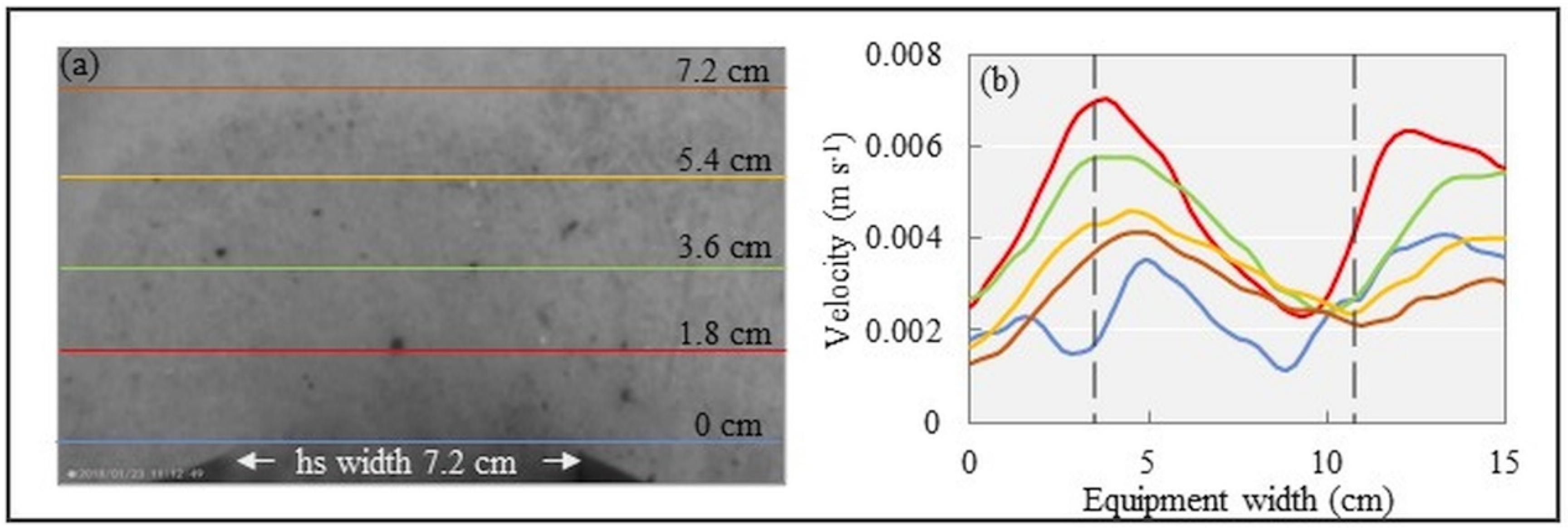
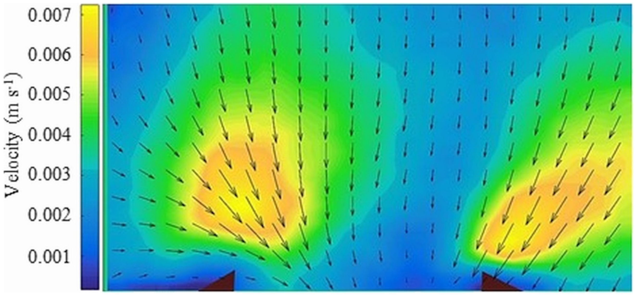
- (a)
- Different modes of locating a Helley–Smith sampler in a riverbed can significantly change the total mass of the sampled sediment, leading to unrealistic estimates of bedload transport. To assess bed-sediment sampling, installing cameras to check the position and flow conditions, as well as the general characteristics of bedload transport and organic matter, is highly recommended.
- (b)
- In the second measurement, we identified temporal variation in sediment transport velocities minute by minute. To carry out better measurements, we recommend sampling over long time periods and repeatedly at each position to reduce uncertainties by increasing sample numbers.
- (c)
- Each piece of equipment, intrusive or non-intrusive, used for estimating bedload transport in sandy rivers has its limits and uncertainties. Performing measurements along with other methodologies, such as moving-bed tests with ADCP or dune tracking is a necessary option.
- (d)
- In addition, from the filming, we were able to qualitatively and quantitatively evaluate the bedload transport and thus improve data analysis in post-processing, whether using PIV or other algorithms.
- (e)
- Future research is recommended in testing both methods (pressure-difference samplers and acoustic methods using ADCPs) simultaneously in either large laboratory flumes or more controlled field experiments.
Author Contributions
Funding
Data Availability Statement
Acknowledgments
Conflicts of Interest
Glossary
| ADCP | Acoustic Doppler Current Profiler |
| Aw | Tropical savannah |
| BM | Bed material |
| BMH-53 | Bed-material sampler |
| D50 | Median particle diameters (mm) |
| D90 | Particle diameter bigger than 90% (mm) |
| e | Sampler efficiency (%) |
| GB | Guariroba Stream Basin |
| HEROS | Hydrology, Erosion, and Sediment Laboratory |
| HS | Helley–Smith (flair ratio equal to 3.47) |
| hs | Helley–Smith handheld (flair ratio equal to 1.95) |
| M | Bedload weight displaced without sampler (Kg) |
| mHS | Sediment weight sampled by Helley–Smith (Kg) |
| PIV | Particle Image Velocimetry |
| Q | Water discharge rate (m3 s m−1) |
| qADCP | Bedload transport rate sampled by ADCP (Kg min−1) |
| qhs | Bedload transport rate sampled by hs (Kg min−1) |
| qHS | Bedload transport rate sampled by HS (Kg min−1) |
| qPIV | Bedload transport rate sampled by PIV (Kg min−1) |
| RTK | Real-Time Kinematics |
| va | Apparent bed-particle velocity (m s−1) |
| vADCP | Bed-particle velocity sampled by ADCP (m s−1) |
| vBT | Bottom-track velocity (m s−1) |
| vDGPS | Differential Global Positioning System velocity (m s−1) |
| vhs | Bed-particle velocity sampled by hs (m s−1) |
| vHS | Bed-particle velocity sampled by HS (m s−1) |
| vm | Depth-averaged vertical velocity (m s−1) |
| vPIV | Bed-particle velocity sampled by PIV (m s−1) |
Appendix A


References
- Atkinson, B.L.; Grace, M.R.; Hart, B.T.; Vanderkruk, K.E.N. Sediment Instability Affects the Rate and Location of Primary Production and Respiration in a Sand-Bed Stream. J. N. Am. Benthol. Soc. 2008, 27, 581–592. [Google Scholar] [CrossRef]
- Larsen, M.C.; Gellis, A.C.; Glysson, G.D.; Gray, J.R.; Horowitz, A.J. Fluvial Sediment in Teh Enviroment: A National Challenge. In Proceedings of the Joint Federal Interagency Conference 2010: Hydrology and Sedimentation for a Changing Future: Existing and Emerging Issues; Cambridge University Press: Cambridge, UK, 2010; 14p. [Google Scholar] [CrossRef]
- USEPA. Causes of Impairment in Assessed Rivers and Streams; USEPA: Washington, DC, USA, 2019.
- Pimentel, D.; Harvey, C.A.; Resosudarmo, P.; Sinclair, K.; Kurz, D.; Mcnair, M.; Crist, S.; Shpritz, L.; Fitton, L.; Saffouri, R.; et al. Environmental and Economic Costs of Soil Erosion and Conservation Benefits. Science 1995, 267, 1117–1123. [Google Scholar] [CrossRef] [PubMed]
- Bagnold, R.A. An Approach to the Sediment Transport Problem From General Physics; Geological Survey Professional Paper 422-I; Cambridge University Press: Cambridge, UK, 1996. [Google Scholar]
- Chen, Y.; Bai, Y.; Xu, D. On the Mechanisms of the Saltating Motion of Bedload. Int. J. Sediment Res. 2017, 32, 53–59. [Google Scholar] [CrossRef]
- Van Rijn, L.C. Sediment Transport, Part I: Bed Load Transport. J. Hydraul. Eng. 1984, 110, 1431–1456. [Google Scholar] [CrossRef]
- Claude, N.; Rodrigues, S.; Bustillo, V.; Bréhéret, J.G.; Macaire, J.J.; Jugé, P. Estimating Bedload Transport in a Large Sand-Gravel Bed River from Direct Sampling, Dune Tracking and Empirical Formulas. Geomorphology 2012, 179, 40–57. [Google Scholar] [CrossRef]
- Gaweesh, M.T.K.; Van Rijn, L.C. Bed-Load Sampling in Sand-Bed Rivers. J. Hydraul. Eng. 1994, 120, 1364–1384. [Google Scholar] [CrossRef]
- Gomez, B.; Church, M. An Assessment of Bed Load Sediment Transport. Water Resour. Res. 1989, 25, 1161–1186. [Google Scholar] [CrossRef]
- Pitlick, J. Variability of Bed Load Measurement. Water Resour. Res. 1988, 24, 173–177. [Google Scholar] [CrossRef]
- Vericat, D.; Church, M.; Batalla, R.J. Bed Load Bias: Comparison of Measurements Obtained Using Two (76 and 152 Mm) Helley-Smith Samplers in a Gravel Bed River. Water Resour. Res. 2006, 42, W10423. [Google Scholar] [CrossRef]
- Gomez, B. Bedload Transport. Earth Sci. Rev. 1991, 31, 89–132. [Google Scholar] [CrossRef]
- Gray, J.R.; Laronne, J.B.; Marr, J.D.G. Bedload-Surrogate Monitoring Technologies; U.S. Geological Survey Scientific Investigations Report; U.S. Geological Survey: Reston, VA, USA, 2010; Volume 5091, pp. 1–37.
- Einstein, H.A. The Bed-Load Function for Sediment Transportation in Open Channel Flows; United States Department of Agriculture, Soil, and Conservation Service: Portland, OR, USA, 1950; p. 1026.
- Kalinske, A.A. Movement of Sediment as Bed Load in Rivers. Trans. Am. Geophys. Union 1947, 28, 615–620. [Google Scholar]
- Meyer-Peter, E.; Muller, R. Formulas for Bed-Load Transport. Int. Assoc. Hydraul. Struct. Res. 1948. Available online: https://repository.tudelft.nl/record/uuid:4fda9b61-be28-4703-ab06-43cdc2a21bd7 (accessed on 22 August 2024).
- Gomez, B.; Naff, R.L.; Hubbell, D.W. Temporal Variations in Bedload Transport Rates Associated with the Migration of Bedforms. Earth Surf. Process. Landforms 1989, 14, 135–156. [Google Scholar] [CrossRef]
- Gray, J.R.; Simões, F.J.M. Estimating Sediment Discharge. In Sedimentation Engineering—Processes, Measurements, Modeling, and Practice: American Society of Civil Engineers Manuals and Reports on Engineering Practice; United States Department of the Interior, Geological Survey-Water Resources Division: Reston, VA, USA, 2008; pp. 1067–1088. [Google Scholar] [CrossRef]
- Gaeuman, D.; Jacobson, R.B. Acoustic Bed Velocity and Bed Load Dynamics in a Large Sand Bed River. J. Geophys. Res. Earth Surf. 2006, 111, 1–14. [Google Scholar] [CrossRef]
- Jamieson, E.C.; Asce, S.M.; Rennie, C.D.; Asce, M.; Jacobson, R.B.; Townsend, R.D. Evaluation of ADCP Apparent Bed Load Velocity in a Large Sand-Bed River: Moving versus Stationary Boat Conditions. J. Hydraul. Eng. 2011, 137, 1064–1072. [Google Scholar] [CrossRef]
- Villard, P.V.; Church, M.A.; Kostaschuk, R. Estimating Bedload in Sand-Bed Channels Using Bottom Tracking from an Acoustic Doppler Profiler. In Fluvial Sedimentology VII; Blackwell Publishing Ltd.: Malden, MA, USA; Oxford, UK; Carlton, VIC, Australia, 2005; pp. 197–209. [Google Scholar] [CrossRef]
- Latosinski, F.; Nicolás, R.; Guerrero, M.; Amsler, L.; Vionnet, C. The ADCP’s Bottom Track Capability for Bedload Prediction: Evidence on Method Reliability from Sandy River Applications. Flow Meas. Instrum. 2017, 54, 124–135. [Google Scholar] [CrossRef]
- Rennie, C.D.; Millar, R.G.; Church, M.A. Measurement of Bed Load Velocity Using an Acoustic Doppler Current Profiler. J. Hydraul. Eng. 2002, 128, 473–483. [Google Scholar] [CrossRef]
- Rennie, C.D.; Villard, P.V. Site Specificity of Bed Load Measurement Using an Acoustic Doppler Current Profiler. J. Geophys. Res. 2004, 109, F03003. [Google Scholar] [CrossRef]
- Conevski, S.; Guerrero, M.; Ruther, N.; Rennie, C.D.; Asce, M. Laboratory Investigation of Apparent Bedload Velocity Measured by ADCPs under Different Transport Conditions. J. Hydraul. Eng. 2019, 145, 04019036. [Google Scholar] [CrossRef]
- Conevski, S.; Guerrero, M.; Rennie, C.D.; Ruther, N. Towards an Evaluation of Bedload Transport Characteristics by Using Doppler and Backscatter Outputs from ADCPs. J. Hydraul. Res. 2021, 59, 703–723. [Google Scholar] [CrossRef]
- Conevski, S.; Guerrero, M.; Winterscheid, A.; Faltis, D.; Rennie, C.D.; Ruther, N. Analysis of the Riverbed Backscattered Signal Registered by ADCPs in Different Bedload Transport Conditions–Field Application. J. Hydraul. Res. 2023, 61, 532–551. [Google Scholar] [CrossRef]
- Frings, R.M.; Vollmer, S. Guidelines for Sampling Bedload Transport with Minimum Uncertainty. Sedimentology 2017, 64, 1630–1645. [Google Scholar] [CrossRef]
- Kostaschuk, R.; Best, J.; Villard, P.; Peakall, J.; Franklin, M. Measuring Flow Velocity and Sediment Transport with an Acoustic Doppler Current Profiler. Geomorphology 2005, 68, 25–37. [Google Scholar] [CrossRef]
- Helley, E.J.; Smith, W. Development and Calibration of a Pressure-Difference Bedload Sampler; USGS Open-File Report; United States Department of the Interior, Geological Survey-Water Resources Division: Reston, VA, USA, 1971; 18p.
- Edwards, T.E.; Glysson, G.D. Field Methods for Collection of Fluvial Sediment. Tech. Water-Resour. Investig. 1999, 3, 89. [Google Scholar] [CrossRef]
- Gray, J.R.; Schwarz, G.E.; Czuba, J.A.; Strom, K.; Diplas, P.; Survey, U.S.G.; Survey, U.S.G.; Engineering, B.S.; Tech, V.; Tech, V.; et al. Facilities, Data, and Analytical Methods Used to Derive Sand- and Gravel-Trapping Efficiencies for Four Types of Pressure. Differ. Bedload Sampl. 2019, 1993, 1–2. [Google Scholar]
- Marr, J.D.G.; Gray, J.R.; Davis, B.E.; Ellis, C.; Johnson, S. Large-Scale Laboratory Testing of Bedload-Monitoring Technologies: Overview of the StreamLab06 Experiments. 2010, pp. 266–282. Available online: https://api.semanticscholar.org/CorpusID:110130184 (accessed on 22 August 2024).
- Beschta, R.L. Increased Bag Size Improves Helley-Smith Bed Load Sampler for Use in Streams with High Sand and Organic Matter Transport. Eros. Sediment Transp. Meas. 1981, 133, 17–26. [Google Scholar]
- Druffel, L.; Emmett, W.W.; Schneider, V.R.; Skinner, J.V. Laboratory Hydraulic Calibration of the Helley- Smith Bedload Sediment Sampler; US Geological Survey: Reston, VA, USA, 1976; pp. 76–752.
- Billi, P. Flash Flood Sediment Transport in a Steep Sand-Bed Ephemeral Stream. Int. J. Sediment Res. 2011, 26, 193–209. [Google Scholar] [CrossRef]
- Boyer, C.; Roy, A.G.; Best, J.L. Dynamics of a River Channel Confluence with Discordant Beds: Flow Turbulence, Bed Load Sediment Transport, and Bed Morphology. J. Geophys. Res. Earth Surf. 2006, 111, 1–22. [Google Scholar] [CrossRef]
- Kasvi, E.; Vaaja, M.; Kaartinen, H.; Kukko, A.; Jaakkola, A.; Flener, C.; Hyyppä, H.; Hyyppä, J.; Alho, P. Geomorphology Sub-Bend Scale Flow—Sediment Interaction of Meander Bends—A Combined Approach of Fi Eld Observations, Close-Range Remote Sensing and Computational Modelling. Geomorphology 2015, 238, 119–134. [Google Scholar] [CrossRef]
- Makaske, B.; Smith, D.G.; Berendsen, H.J.A.; de Boer, A.G.; van Nielen-Kiezebrink, M.F.; Locking, T. Hydraulic and Sedimentary Processes Causing Anastomosing Morphology of the Upper Columbia River, British Columbia, Canada. Geomorphology 2009, 111, 194–205. [Google Scholar] [CrossRef]
- Venditti, J.G.; Church, M.; Bennett, S.J. Morphodynamics of Small-Scale Superimposed Sand Waves over Migrating Dune Bed Forms. Water Resour. Res. 2005, 41, 1–14. [Google Scholar] [CrossRef]
- Bunte, K.; Klema, M.; Hogan, T.; Thornton, C. Testing the Hydraulic Efficiency of Pressure Difference Samplers While Varying Mesh Size and Type Technical Committee of the Federal Interagency Sedimentation Project; Colorado State University, Engineering Research Center: Fort Collins, CO, USA, 2017. [Google Scholar]
- Sawadogo, O.; Basson, G.R. 3D fully coupled numerical modelling of local sediment flushing scour at dam bottom outlets for sustainable hydropower operation. In River Sedimentation; CRC Press: Boca Raton, FL, USA, 2017; pp. 1154–1160. [Google Scholar]
- Frank-Gilchrist, D.P.; Penko, A.; Calantoni, J. Investigation of Sand Ripple Dynamics with Combined Particle Image and Tracking Velocimetry. J. Atmos. Ocean Technol. 2019, 35, 2019–2036. [Google Scholar] [CrossRef]
- Gollin, D.; Brevis, W.; Bowman, E.T.; Shepley, P. Performance of PIV and PTV for Granular Flow Measurements. Granul. Matter 2017, 19, 42. [Google Scholar] [CrossRef]
- Lueptow, R.M.; Akonur, A.; Shinbrot, T. PIV for Granular Flows. Exp. Fluids 2000, 28, 183–186. [Google Scholar] [CrossRef]
- Sarno, L.; Carravetta, A.; Tai, Y.; Martino, R.; Papa, M.N.; Kuo, C. Measuring the Velocity Fields of Granular Flows—Employment of a Multi-Pass Two-Dimensional Particle Image Velocimetry (2D-PIV) Approach. Adv. Powder Technol. 2018, 29, 3107–3123. [Google Scholar] [CrossRef]
- Van Scheltinga, R.C.T.; Friedrich, H. Sand Particle Velocities over a Subaqueous Dune Slope Using High-Frequency Image Capturing. Earth Surf. Process. Landf. 2019, 44, 1881–1894. [Google Scholar] [CrossRef]
- Senatore, C.; Wulfmeier, M.; Vlahinić, I.; Andrade, J.; Iagnemma, K. Design and Implementation of a Particle Image Velocimetry Method for Analysis of Running Gear-Soil Interaction. J. Terramech. 2013, 50, 311–326. [Google Scholar] [CrossRef]
- Tsubaki, R.; Baranya, S.; Muste, M.; Toda, Y. Spatio-Temporal Patterns of Sediment Particle Movement on 2D and 3D Bedforms. Exp. Fluids 2018, 59, 93. [Google Scholar] [CrossRef]
- Ermilov, A.A.; Fleit, G.; Conevski, S.; Guerrero, M.; Baranya, S.; Rüther, N. Bedload Transport Analysis Using Image Processing Techniques. Acta Geophys. 2022, 70, 2341–2360. [Google Scholar] [CrossRef]
- Hubbell, D.W. Apparatus and Techniques for Measuring Bedload; U.S. Geological Survey Water-Supply Paper; U.S. Government Publishing Office: Washington, WA, USA, 1964; Volume 1748, p. 74.
- Emmett, W.W. A Field Calibration of the Sediment-Trapping Characteristics of the Helley-Smith Bedlaod Sampler; U.S. Geological survey professional paper; United States Government Printing Office: Washington, WA, USA, 1980; p. 1139.
- Peel, M.C.; Finlayson, B.L.; McMahon, T.A. Long-Term Rates of Mass Wasting in Mesters Vig, Northeast Greenland: Notes on a Re-Survey. Hydrol. Earth Syst. Sci. 2007, 11, 1633–1644. [Google Scholar] [CrossRef]
- Valle Junior, L.C.G.; Rodrigues, D.B.B.; Oliveira, P.T.S. Initial Abstraction Ratio and Curve Number Estimation Using Rainfall and Runoff Data from a Tropical Watershed. Rev. Bras. Recur. Hidr. 2019, 24, 1–9. [Google Scholar] [CrossRef]
- Wagner, C.R.; Mueller, D.S. Comparison of Bottom-Track to Global Positioning System Referenced Discharges Measured Using an Acoustic Doppler Current Profiler. J. Hydrol. 2011, 401, 250–258. [Google Scholar] [CrossRef]
- Rennie, C.D.; Rainville, F. Case Study of Precision of GPS Differential Correction Strategies: Influence on aDcp Velocity and Discharge Estimates. J. Hydraul. Eng. 2006, 132, 225–234. [Google Scholar] [CrossRef]
- Mueller, D.S. QRev—Software for Computation and Quality Assurance of Acoustic Doppler Current Profiler Moving-Boat Streamflow Measurements—User’s Manual for Version 2.8; U.S. Geological Survey Open-File Report 2016-1052; U.S. Geological Survey: Reston, VA, USA, 2016. [CrossRef]
- Thielicke, W.; Stamhuis, E.J. PIVlab—Towards User-Friendly, Affordable and Accurate Digital Particle Image Velocimetry in MATLAB. J. Open Res. Softw. 2014, 2, 30. [Google Scholar] [CrossRef]
- Shavit, U.; Lowe, R.J.; Steinbuck, J.V. Intensity Capping: A Simple Method to Improve Cross-Correlation PIV Results. Exp. Fluids 2007, 42, 225–240. [Google Scholar] [CrossRef]
- Hart, D.P. PIV Error Correction. Exp. Fluids 2000, 29, 13–22. [Google Scholar] [CrossRef]
- Huang, H.; Daribi, D.; Gharibi, M. On Errors of Digital Particle Image Velocimetry. Meas. Sci. Technol. 1997, 8, 1427–1440. [Google Scholar] [CrossRef]
- Keane, R.D.; Adrian, R.J. Theory of Cross-Correlation Analysis of PIV Images. Appl. Sci. Res. 1992, 49, 191–215. [Google Scholar] [CrossRef]
- Westerweel, J.; Scarano, F. Universal Outlier Detection for PIV Data. Exp. Fluids 2005, 39, 1096–1100. [Google Scholar] [CrossRef]
- Carvalho, N.D.O.; Ide, C.N.; do Val, L.A.A.; Rondon, M.A.C.; Barbedo, A.G.A.; Cybis, L.F.d.A. Causas Do Assoeramento Dos Rios Da Bacia Do Alto Paragui e Os Efeitos Decorrentes Nas Cheias. In Proceedings of the VIII Encontro Nacional de Engenharia de Sedimentos, Campo Grande, Brazil, 2–8 November 2008; pp. 1–18. [Google Scholar]


| Reference | Equipment Size (cm) | Particle Size Tested (D50) (mm) | Mean Water Velocity (m s−1) | Efficiency (%) |
|---|---|---|---|---|
| Helley and Smith [31] | n.a 7.62 × 7.62 n.e 19.05 × 10.80 n.t 1.27 | 1.15 | 0.51–1.29 | 122–262 a,c |
| Druffel et al. [36] | n.a 7.62 × 7.62 n.e 19.05 × 10.80 n.t 1.27 | 0.2, 1.2 and 10 | 0.83–1.33 | Undetermined a,c |
| Druffel et al. [36] | n.a 15.24 × 15.24 n.e 38.10 × 21.59 n.t 1.27 | 0.2, 1.2 and 10 | 0.72–1.00 | 1.54 a,d |
| Emmett [53] | n.a 7.62 × 7.62 n.e 19.05 × 10.80 n.t 1.27 | 0.25–0.50 0.5–16 | 0.57–1.42 | 150 b,c 92.6 b,c |
| Beschta [35] | n.a 7.6 × 7.6 | 0.2–0.5 | 0.75–1.24 | 76 a,c |
| Pitlick [11] | n.a 7.62 × 7.62 n.e 19.05 × 10.80 n.t 1.5 | 1 | - | 100 |
| Pitlick [11] | n.a 7.62 × 7.62 n.e 19.05 × 10.80 n.t 6.3 | 1 | - | 50 |
| Vericat et al. [12] | n.a 7.62 × 7.62 n.a 15.24 × 15.24 | 21 | 1.5–2 | Undetermined b,c |
| Bunte et al. [42] | n.a 15.24 × 30.48 n.a 10.66 × 20.32 n.a 7.62 × 7.62 | - | 0.45; 0.76; 1.07 | 108–115 a,d 101–110 a,d 93–102 a,d |
| Velocity Profile and Streamflow | Bedload and Bed-Material Sampler | Time Recording (Minute) | Image Resolution (Pixel) | Frame Rate | Frame Size (cm) | |
|---|---|---|---|---|---|---|
| 1st Measurement | Mechanical current meter | hs and BMH-53 | 15 | 3840 × 2160 | 24 | 15.0 × 8.4 |
| 2nd Measurement | ADCP | hs, HS, and BMH-53 | 15 | 2704 × 2032 | 60 | 35.0 × 26.3 |
| Depth-Averaged Vertical Velocity (m s−1) | va (m s−1) | D50 (%) | D50 (mm) | σg | Sk | Degree of Sorting | ||
|---|---|---|---|---|---|---|---|---|
| 1st Measurement | BM hs | 0.66 | - | 95.60 90.03 | 0.45 0.34 | 0.12 0.39 | 0.34 0.87 | 0.33 1.03 |
| 2nd Measurement | BM | 0.64 | 0.014 | 93.29 | 0.44 | 0.35 | 1.00 | 0.49 |
| hs | 95.65 | 0.45 | 0.18 | 0.49 | 1.36 | |||
| HS | 64.22 | 0.34 | 0.43 | 0.87 | 0.93 |
| Measurement | Camera Distance (cm) | Resolution (px) | Particles per IW | Density (Particles/IW) | IW Dimensions (px) |
|---|---|---|---|---|---|
| 1st | 15 | 3840 × 2160 | 11 | Sufficient | 256 × 256, 28 × 128, 64 × 64 |
| 2nd | 23 | 2704 × 2032 | 6 | Sufficient | 256 × 256, 28 × 128, 64 × 64 |
| First Measurement | Second Measurement | |
|---|---|---|
| D50 (mm) | 0.45 | 0.44 |
| D90 (mm) | 0.49 | 0.49 |
| vm (m s−1) | 0.83 | 0.80 |
| Q (m3 s m−1) | 0.98 | 0.88 |
| vhs (m s−1) | * | 0.02 |
| vHS (m s−1) | * | 0.003 |
| vADCP (m s−1) | * | 0.014 |
| vPIV (m s−1) | 0.0028 | 0.0145 |
| qhs (Kg min−1) | 1.23 | 1.92 |
| qHS (Kg min−1) | * | 0.19 |
| qADCP (Kg min−1) | * | 1.19 |
| qPIV (Kg min−1) | 0.23 | 1.23 |
| Efficiency (%) | 534.78 a | 156.10 a; 15.45 b; 96.75 c |
Disclaimer/Publisher’s Note: The statements, opinions and data contained in all publications are solely those of the individual author(s) and contributor(s) and not of MDPI and/or the editor(s). MDPI and/or the editor(s) disclaim responsibility for any injury to people or property resulting from any ideas, methods, instructions or products referred to in the content. |
© 2025 by the authors. Licensee MDPI, Basel, Switzerland. This article is an open access article distributed under the terms and conditions of the Creative Commons Attribution (CC BY) license (https://creativecommons.org/licenses/by/4.0/).
Share and Cite
Pereira, R.B.; Carvalho, G.A.; Bleninger, T.; Zamboni, P.A.P.; Wosiacki, L.; Gonçalves, F.V.; Janzen, J.G. Particle Image Velocimetry Analysis of Bedload Sampling in a Sand-Bed River. Fluids 2025, 10, 165. https://doi.org/10.3390/fluids10070165
Pereira RB, Carvalho GA, Bleninger T, Zamboni PAP, Wosiacki L, Gonçalves FV, Janzen JG. Particle Image Velocimetry Analysis of Bedload Sampling in a Sand-Bed River. Fluids. 2025; 10(7):165. https://doi.org/10.3390/fluids10070165
Chicago/Turabian StylePereira, Rodrigo B., Glauber A. Carvalho, Tobias Bleninger, Pedro A. P. Zamboni, Liege Wosiacki, Fábio V. Gonçalves, and Johannes Gérson Janzen. 2025. "Particle Image Velocimetry Analysis of Bedload Sampling in a Sand-Bed River" Fluids 10, no. 7: 165. https://doi.org/10.3390/fluids10070165
APA StylePereira, R. B., Carvalho, G. A., Bleninger, T., Zamboni, P. A. P., Wosiacki, L., Gonçalves, F. V., & Janzen, J. G. (2025). Particle Image Velocimetry Analysis of Bedload Sampling in a Sand-Bed River. Fluids, 10(7), 165. https://doi.org/10.3390/fluids10070165