AI-Driven Surrogate Model for Room Ventilation

Abstract

The control of ventilation systems is often performed by automatic algorithms which often do not consider the future evolution of the system in its control politics. Digital twins allow system forecasting for a more sophisticated control. This paper explores a novel methodology to create a Machine Learning (ML) model for the predictive control of a ventilation system combining Computational Fluid Dynamics (CFD) with Artificial Intelligence (AI). This predictive model was created to forecast the temperature and humidity evolution of a ventilated room to be implemented in a digital twin for better unsupervised control strategies. To replicate the full range of annual conditions, a series of CFD simulations were configured and executed based on seasonal data collected by sensors positioned inside and outside the room. These simulations generated a dataset used to develop the predictive model, which was based on a Deep Neural Network (DNN) with fully connected layers. The model’s performance was evaluated, yielding final average absolute errors of 0.34 degrees Kelvin for temperature and 2.2 percentage points for relative humidity. The presented results highlight the potential of this methodology to create AI-driven digital twins for the control of room ventilation.

1. Introduction

Nowadays, multiple industries rely on a wide variety of automatic control strategies to control different processes and facilities. Among all these strategies, some of them are based on forecasting the future behavior of the system based on sparse real-time information available through sensors. Digital twins can be found in the previous group, which employ real-time data from interest variables and system actuators gathered by sensors to replicate the dynamical behavior of the system under study. The core simulator of a digital twin can be a mathematical model ranging from analytical models to sophisticated systems of partial differential equations solved by proper numerical methods.

This virtual simulation serves as a base to analyze the dynamics of the system, optionally comparing it with historical data, to implement optimized control strategies. The representation of the physical system can also be used to establish a comprehensive analysis of the real system [1]. In an era where a massive amount of data is accessible and large computing clusters are readily available, creating in-house digital twins to control systems has become not only feasible but a growing trend across diverse industries. They can be applied to traditional sectors such as agriculture [2], as well as industrial processes [3] and manufacturing [4]. Indeed, they can be useful in complex workflow like urban planning [5], showcasing their versatility and value in driving operational efficiency and innovation [6].

To implement a digital twin in a system where one or more fluids are involved, the modeling core can be deployed with Computational Fluid Dynamic (CFD) simulations, since they implement the set of equations that model the behavior of such fluids and their interactions with external bodies and surfaces. The use of CFD simulations to model room ventilation is not new, and it is possible to find reviews analyzing papers based on CFD for the past decades [7,8]. Most of the works conducted in this area aim at reproducing in a virtual environment a ventilated room. This reproduction allows one to understand the effects of the different elements of the ventilation system to improve its design and performance as well as increasing room comfort [9].

Furthermore, it is possible not only to model the hydrodynamics and heat transfer of such systems, but also to model the evaporation and condensation of water in different scenarios. Different works can be cited in this field, and it is of interest to mention [10], where energy transfer and psychrometric variables are included to model the condensation of water vapor, validating the work with experimental data. In [11], a similar study is conducted, using a pilot reactor with controlled conditions to validate the simulations of the water condensation. The aforementioned works study reduced cases to test their different models, whereas in [12], an underground facility has been modeled with CFD, evaluating different air conditioning systems to avoid water condensation. Some works can be found regarding water evaporation using CFD simulations. In [13], an indoor swimming pool facility has been modeled, including the ventilation system, to study the evaporation and transport of water vapor. Similarly interesting works can be found in [14,15,16]. On a more detailed level, [17,18] study the effect of convective flow and air conditions on the evaporation rate of indoor swimming pools. The present paper implements an evaporation source similar to the one used by Elazm et al. [19]. They study the effect of air velocity at the water interphase on water evaporation, with a source term proposed by the American Society of Heating, Refrigerating, and Air-Conditioning Engineers (ASHRAE) [20].

The cited works focus mainly on essential phenomena related to water vapor generation or condensation independently. Several works can be found where only one of both effects is included, depending on the scope of the study or the characteristics of the system. One of the distinctive features of the present paper is that it includes both effects as they play an important role in the studied problem.

Despite the great advantages that CFD simulations may provide, the integration of such tools into ventilation control is usually suboptimal. As an illustrative example, in [21], CFD simulations are included in a control loop with a PID controller for room ventilation. For small systems where the time required to obtain a converged simulation result is minor compared with the inertia of the system, these kinds of proposals are realizable. Unfortunately, this may be rather the exception than the norm, typically requiring these simulations several hours to finish and being unfit to be implemented in real-time controls.

Especially for digital twins, the key requirement is to reproduce the dynamics of the system in real time; that is, the predicted state of the system (in terms of the spatial distribution of velocity, temperature, and relative humidity) has to be known prior to the occurrence of that state so that a control strategy can be studied and implemented. This requirement strongly limits the implementation of CFD simulations in digital twins, since the necessary time to complete such simulations can span from minutes to days depending on the dimensions and complexity of the system.

To solve this problem, a novel methodology is proposed and studied in the present work, creating and training an Artificial Intelligence (AI) model using physics-informed data from CFD simulations to learn the behavior of a ventilated room with presence of water vapor, approximating future states of the system in milliseconds. To the authors’ best knowledge, the use of AI to predict the state variables of a ventilated room based on sensor data is new, a recent work from Quang et al. [22] being the closest one. Quang uses different ML models trained with CFD simulations to predict the velocity and temperature distribution in an indoor building caused by natural convection, although there is no prediction of the relative humidity. The approach proposed in the present work for ventilated rooms with presence of water vapor bridges the gap between detailed CFD analysis and practical, actionable insights, allowing the implementation of a digital twin for automated ventilation control.

The integration of CFD with AI is a state-of-the-art field with lots of research branches [23] that can encompass simple regression models that predict CFD results to more complex systems that control machines with the help of Deep Reinforcement Learning (DRL). The reason behind its growing spread in multiple areas of technology is due to its predictive speed and computational efficiency, along with the ability to scale large datasets and complex systems, making them suitable for various real-world applications. Some researches remark the use of Physics-Informed Neural Networks (PINNs) [24,25,26]. Although their implementation provides better inferences fulfilling physical governing equations, they are mostly restricted to general conservation equations. However, in the present case, the problem requires to predict transported species with complex sink and source terms. The inclusion of such specific equations is not yet clear for a PINN, and thus, this approach has been discarded for the present work.

It is important to remark that the deployment of digital twins implementing AI models is a research topic in development, and there exist a wide variety of control systems based on this solution, tackling problems for many different industries. A reader willing to explore previous works in this area may be referred to the following review [27]. Despite the considerable amount of work performed to implement digital twins with AI models, and the amount of research conducted in the previous years coupling AI with CFD simulations, to the knowledge of the present authors, almost no work has been carried out to use these CFD–AI models to create a digital twin. To put a number on this statement, in another review [28], 149 studies have been analyzed, finding only one work where the use of CFD-based AI models is integrated into a digital twin. In this mentioned study [29], the authors use AI models based on CFD simulations to predict simple variables representative of the system in order to build a digital twin. Moreover, there is an increasing interest not only in digital twins but also in the surrogate models they use with different architectures and approaches [30,31] or even in the promising field of Deep Learning explainability, where they try to explain the different behaviors of the fluid in CFD [32]. Furthermore, hybrid CFD solvers where ML helps to accelerate the final converged solution for steady-state problems or skips timesteps in transient ones is also an increasing interest in the research community [33,34].

To wrap up, the present study combines different research problems found in the bibliography into a joint study. Regarding the modeling of ventilated rooms, in this work, a CFD model of a complex ventilated room will be obtained, both incorporating the phenomenon of water evaporation and condensation. This poses an extra challenge compared with previous works, as now both opposing phenomena need to be included and the results will be influenced by its equilibrium. In addition, data from sensors needs to be gathered around a year to be able to create a suitable and realistic dataset to train the surrogate model. Furthermore, it is a considerable challenge to train a predictive generative model capable of inferring the complete state of a complex system using only few input data. Combined with that, another problem of the present research work is to select the best suitable sensor position inside the room to optimize the predictive performance of the model by maximizing the quality of the input data.

With the aforementioned research problems presented, the novelty of this work lies in exploring the methodology of using a CFD–AI surrogate model to approximate the complete state of a ventilated room based on real-time data from sensors. This predictive tool can be envisioned as a computing core to build a digital twin of the ventilated room to guide the control strategies in advanced ventilation systems. By taking into account the 3D state of the system, deeper spatial analysis will be possible, enabling the study of more complex and accurate actuation rules, ultimately leading to more efficient operational uses.

The following sections are devoted to describing the methodology followed in the present work and the results obtained. Materials and Methods introduces the ventilated room studied in this work, describing its ventilation systems and the main variables describing its operational state. Furthermore, the CFD models used in the simulations are listed, and the mesh generation process and configuration of boundary conditions are presented. Finally, the architecture of the CFD–AI surrogate model is described and the optimization process depicted. In Results, the main findings of the work are shown, illustrated with one example case simulation for the CFD results, and one predicted case for the accuracy of the predictive model. The overall assessment of the CFD–AI model is also included for completion. Last, sections Discussion and Conclusions gather the main interpretations of the findings and wrap up some final comments.

2. Materials and Methods

In this section, all details of the methodology used to carry out the present research work are described. First, the case study is described, presenting the facility where this work was developed. From this case, the set of variables that permits a complete characterization of the facility is identified and described. Representative sensor data is provided, and the generation of the dataset is given. To continue, the CFD model used to simulate the described domain is depicted, presenting all relevant equations and simplifications. Then, the generated mesh is shown, along with the description of the configuration for the relevant boundary conditions of the system. Finally, the architecture of the CFD–AI surrogate model is introduced, showing the point grid used to extract the data from the CFD simulations to train the model. The stages for the optimization of the CFD–AI model are depicted.

2.1. Context and Facility Description

The present manuscript leverages AI to create a surrogate model for the ventilation of a specific room within the Oceanogràfic (https://www.oceanografic.org/), a public aquarium and marine complex situated in the Jardí del Túria in the city of València. Oceanogràfic is a large facility composed of multiple underground galleries and connected rooms. To ensure the well-being of the marine fauna, a complex of underground chambers with technical equipment extends next to each aquarium, controlling the conditions of the water for each environment while purifying and cleaning it from impurities. These technical rooms contain technical equipment (pumps, mixers, control electronics, etc.) and are usually located behind the aquariums, in direct contact with them by windows and chambers above the water level. To develop the presented work, only a room with one connection to the main gallery was selected to work with.

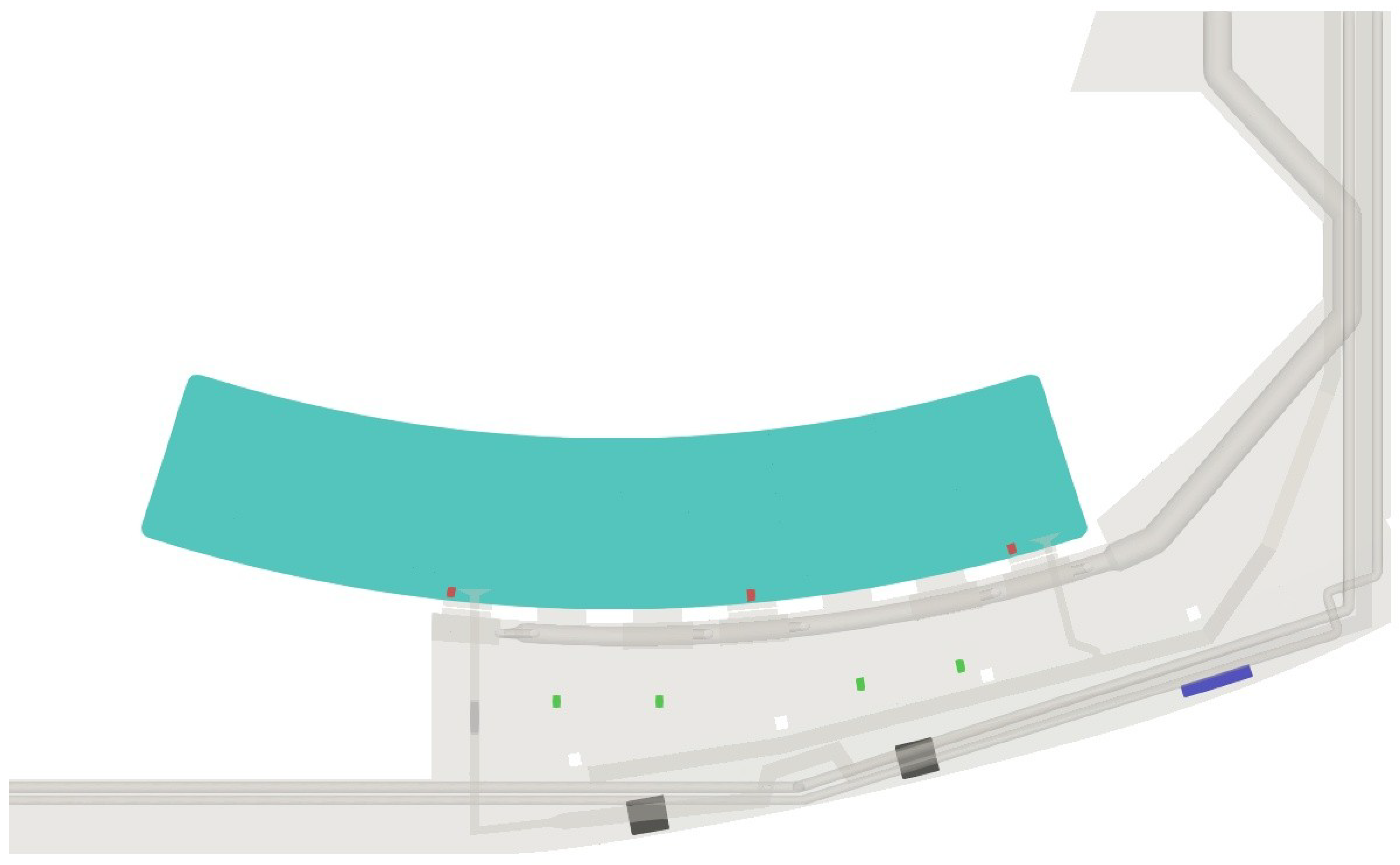
To represent and describe the selected space for the study, Figure 1 and Figure 2 present a 2D and 3D view of the studied room. In Figure 1, two regions can be appreciated: one at ground level, named technical room from now on, and one elevated from the ground that communicates with a water surface (light blue in the scheme), which will be named chamber. Both regions communicate with a set of apertures, named windows from now on, that must remain opened for maintenance purposes. 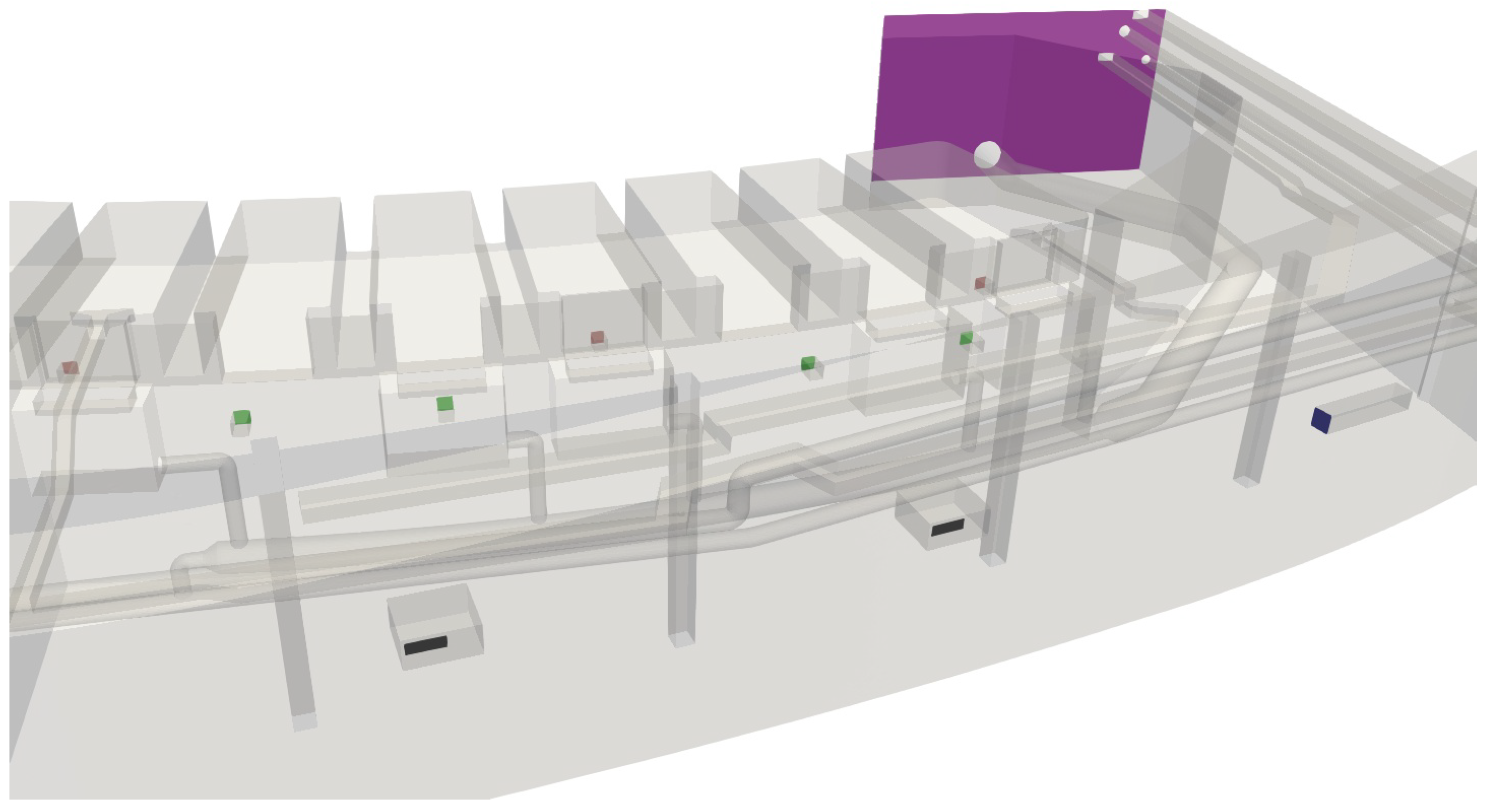In Figure 2, the purple surface represents the only connection of the room with the gallery and will be referred to as swap surface.

Without proper ventilation, the water vapor generated at the water surface would be transported from the chamber to the technical room by means of diffusion and natural air currents. When psychrometric conditions are unfavorable, the evaporation rate rises, resulting in subsequent condensation on the walls, roof, and technical equipment. This condensation is responsible for increased corrosion on devices causing apparatus malfunction and structural damages.

To palliate these problems and to ensure air renovation, ventilation circuits are installed in the rooms, consisting of a supply circuit and an exhaust circuit. Furthermore, in the room object of the present study, a drying circuit was implemented to provide extra dehumidification. The locations for the ventilation grilles are illustrated in Figure 1. The supply circuit grilles are painted dark blue, the exhaust circuit grilles red, the intake grilles of the drying circuit are black (corresponding to two dehumidifiers), and the discharge grilles are green. For the sake of simplicity, only the final section of the ventilation circuits has been modeled, since other circuits and pipes are already inside the room and act as obstacles for the air. Figure 2 shows a 3D view of the simulated domain, with the grilles acting as inlets (discharge) or outlets (intake) colored according to each circuit. Finally, the swap surface is colored in purple (note that the air flow can go in both directions across this surface depending on the flow conditions).

In this configuration, the supply circuit introduces fresh air from the exterior of the facility into the technical room, causing the main air current in the domain of the study. Note that the temperature and humidity of the supplied air depends on external meteorological conditions (typically between 60% and 90%). The exhaust system is designed to remove stale and humid air from the chamber. By extracting air from this location, the air flow through the windows is directed towards the chamber. This prevents humidity diffusion into the technical room, thus maintaining optimal air quality and the buildup of excess moisture in its interior. When the net flow between exhaust and supply is positive, i.e., exhaust flow is greater than the supply one, the defect of air is covered by an inflow from the gallery via the swap surface. When the net flow is negative, the excess of air from the supply circuit exits the room via the swap surface to the gallery. Finally, the drying circuit reduces the moisture content of the air supplied from the exterior and the gallery. Each dehumidifier draws in humid air, cooling it to condense the moisture, and then reheats the air before releasing it through the discharge drying grilles. This process ensures that the air remains dry and comfortable in the technical room. The resulting dry air is injected towards the windows to further prevent moisture diffusion into the technical room. Therefore, the combination of the different ventilation systems leads to multiple behaviors and situations that need to be taken into account and have their representation on the generated data used to train the predictive model.

2.2. CFD Model

The CFD simulations forming the training dataset were conducted using OpenFOAM v2306, an open-source software widely employed in academia and research for its flexibility and the ability to integrate custom code to enhance its functionality. The solver buoyantBoussinesqSimpleFoam was used, a choice motivated by the expected low variation of air density due to the low variations of temperature in the domain. It was also assumed that the low pressure changes due to buoyant and velocity change effects would produce almost negligible changes on the density. In such cases, the Boussinesq approximation can be used, assuming a linear variation of air density with temperature as given in Equation (1):

$$\rho ={\rho }_0[1-\beta (T-T_{ref})],$$

(1)

where $\rho$ is the air density, ${\rho }_0$ is the reference density at $T_{ref}$ temperature, $\beta$ is the thermal expansion coefficient ($3\times {10}^{-3}$ ${\mathrm{K}}^{-1}$), and $T_{ref}$ is the reference temperature (300 K).

Under these assumptions, according to Ferziger and Peric [35], the density can be treated as constant in the unsteady and convection terms, but treated as variable in the gravitational term. As the density is considered constant for the majority of the terms, and the velocities are expected to be low, an incompressible approach for the air can be used. Thus, the Averaged Navier–Stokes equation is modified as shown below:

$$\nabla ·\left(\overrightarrow{u}\overrightarrow{u}\right)=-{\displaystyle \frac{1}{{\rho }_0}}\left(\nabla p-\rho \overrightarrow{g}\right)+\nabla ·\left({\nu }_{Eff}\nabla \overrightarrow{u}\right).$$

(2)

With ${\nu }_{Eff}$, the modeled effective viscosity is computed as ${\nu }_{Eff}=\nu +{\nu }_t$, with ${\nu }_t$ being the turbulent viscosity modeled with the corresponding turbulence model. The time derivative term has been removed, as the converged steady-state solution is desired to train the model.

Several works devoted to simulating the ventilation of rooms with large volumes as the one in the present work use the k–$\epsilon$ model or similar variants [9,10,11,12,13] due to limitations in the computational resources required to properly resolve the boundary layer. It is important to stress the fact that the present work is not devoted to investigating the effect of the turbulence modeling on the evaporation and condensation rates. Rather, its main focus lays on obtaining a surrogate model to predict the approximate equilibrium state of a ventilated room in pursuit of being implemented in a control algorithm. Expecting low velocity gradients in the majority of the domain, and being aware that the computational resources required to resolve the boundary layer with more sophisticated turbulence models, the k–$\epsilon$ turbulence model has been used. This model offers a good tradeoff between accuracy and resource efficiency.

To provide closure to the system of equations, the energy conservation equation has been modified and rearranged under the simplifications of incompressible flow and Boussinesq approach as

$$\nabla ·\left(T\overrightarrow{u}\right)=\nabla ·\left(\left({\displaystyle \frac{\nu }{Pr}}+{\displaystyle \frac{{\nu }_t}{P{r}_t}}\right)\nabla \overrightarrow{u}\right)+S_T.$$

(3)

where $Pr$ is the Prandtl number (taken as 0.7), $P{r}_t$ the turbulent Prandtl number (taken as 0.85), and S a source term of energy coming from radiation, convection, or conduction from external sources or boundary surfaces.

To model the presence of relative humidity, the simulated fluid was chosen to be dry air, and the water vapor was transported as a scalar variable over the air. This simplification was made after studying the error committed in density estimation by not accounting for the mass of evaporated water present in the air. The extreme case would be at high temperature ($40$°C in summer) with maximum saturation of water vapor. In this situation, the difference of density between dry air and moist air would be of a $2.75\%$. It is assumed that this error is acceptable to generate the results used to test the proposed methodology of this work. The transport of relative humidity is governed according to the following equation:

$$\nabla ·\left(w\overrightarrow{u}\right)=\nabla ·\left(\left({\displaystyle \frac{\nu +{\nu }_t}{Sct}}\right)\nabla w\right)+S_w,$$

(4)

with w being the specific humidity (${\mathrm{kg}}_{\mathrm{H}2\mathrm{O}}/{\mathrm{m}}^3$), while $\nu$ and ${\nu }_t$ stand for the kinematic and turbulent kinematic viscosity, respectively, and $Sct$ is the Schmidt number. Finally, $S_w$ represents a source/sink term for the specific humidity, being a source when evaporation from the water surface occurs, and a sink when condensation happens in the walls of the domain. The experimental correlation used to model the source/sink term of water vapor is a variant of Carrier’s empirical correlation [36] included in the ASHRAE’s Application Handbook [20]. As this correlation does not consider the effect of vapor density difference, it tends to over-predict the evaporation rate. To improve its accuracy, Smith et al. [37] proposed a correction for indoor and outdoor swimming pools, multiplying Carrier’s correlation by 0.76. Therefore, the final empirical correlation used in Equation (5) was

$${\varphi }_w=A·0.76(0.08893+0.07835v){\displaystyle \frac{(P_{v,s}-RH·P_{v,inf})}{h_{fg}}},$$

(5)

where A is the surface area of the patch where the condensation/evaporation occurs, v is the air velocity next to the water surface, and $P_{v,s}$ is the saturated vapor pressure at the surface temperature, whereas $P_{v,inf}$ is the saturated vapor pressure at air temperature at the cell center. $RH$ is the relative humidity and $h_{fg}$ is the latent heat of vaporization. The previous equation relates to the total amount of vapor exchange by a surface [kg/s]; to implement the source term $S_w$, it is necessary to divide by the cell volume, resulting in $S_w={\varphi }_w/V_{cell}$.

2.3. Studied Variables and Sensor Data

The prediction of the steady-state configuration of the room characteristics needs the knowledge of a limited set of variables. These variables can be separated into three subsets: distribution of psychrometric variables in the initial state (spatial distribution of temperature and relative humidity), psychrometric variables in the boundaries of the domain (swap surface and ventilation grilles), and the values for the actuators that activate the flow in the three circuits (supply, exhaust, and drying).

The knowledge of the distribution of the psychrometric variables in the initial state is a cumbersome task, as the values of temperature and relative humidity present changes across the domain. Consequently, one would need a considerable amount of data to accomplish this requirement. However, the structure of these fields is determined by the fluid dynamics inside the volume, so the resulting distribution might be properly described by a reduced number of sensors. In this approach, 4 sampling locations were selected to account for the initial conditions. This amount of sensors is not the result of a casual choice, but because of technical limitations. This is so because only four more sensors were available and installed in the studied room. It is understood by the authors that more sensors would increase the predictive accuracy of the NN; this is a limitation of this work. The exact positions of the rest of the sensors were not known a priori, but resulted from the analysis of the CFD results (the procedure is detailed in Section 2.5.3).

The knowledge of the psychrometric variables in the boundary conditions is also required. The temperature and relative humidity of the supply discharge play a central role, as they are related to the main air current in the domain. Also, the knowledge of these magnitudes in the discharge drying grilles is of primary importance, as they represent the main source of air treatment in the domain. The temperatures in the walls are also important as they have a strong influence in the condensation. Finally, the psychrometric conditions at the swap surface are relevant for those cases when there is a net negative flow into the room. Due to its importance on the psycrhometric conditions in the vicinity of the room, one sensor from the set destined to monitoring the internal state of the room was placed near the swap surface, and its location was fixed.

To sum up, the necessary variables regarding psychrometric conditions are as follows:

• Room temperature at 3 locations (K);
• Room humidity at the same 3 locations (%);
• Supply temperature (K);
• Supply relative humidity (%);
• Swap temperature (K);
• Swap relative humidity (%);
• Dehumidifier temperature (K);
• Dehumidifier relative humidity (%);
• Wall temperature (K).

Regarding the actuators of the ventilation system, three levels of functioning have been defined for each circuit. The supply and exhaust circuits have a frequency converter to control the air flow between 50% and 100% of its nominal flow ($3000{\mathrm{m}}^3/\mathrm{h}$). To reduce the amount of dataset combinations, three states where considered for both the supply and exhaust fans: switched off, 50% of its maximum flow rate, and its maximum flow rate. The surrogate model should be able to properly predict the results for any flow rate between 50% and the maximum. The dehumidifiers have only two operational points: on and off, with a constant flow rate of $1500{\mathrm{m}}^3/\mathrm{h}$ per dehumidifier. Combining both machines, the possible flow rates for the drying circuit are 0, 1500, and 3000 ${\mathrm{m}}^3/\mathrm{h}$. To sum up, the necessary variables regarding actuators are

• Supply flow rate (${\mathrm{m}}^3/\mathrm{h}$);
• Exhaust flow rate (${\mathrm{m}}^3/\mathrm{h}$);
• Drying flow rate (${\mathrm{m}}^3/\mathrm{h}$).

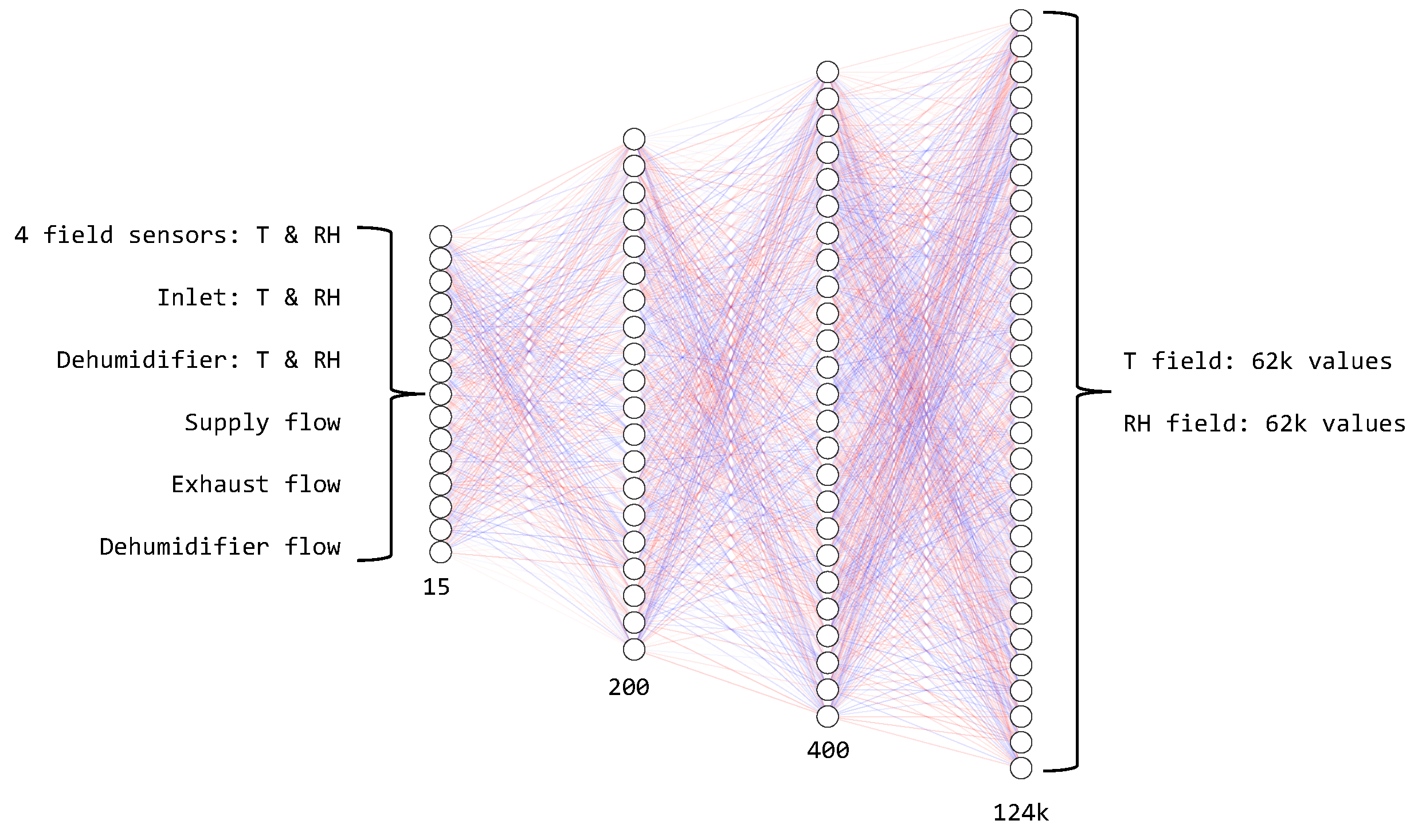
From this analysis, the set of 15 variables forming the inputs of the predictive model was 4 temperatures and 4 relative humidities for the initial conditions and swap surface, the temperature and humidity of the supply and drying circuits, and the three flow rates for the actuators.

Note that the wall temperature has not been considered as an input for the predictive model, which is mostly motivated by the lack of proper experimental data. The studied domain presents a total area covered by walls of roughly $2300{\mathrm{m}}^2$; this represents a great complexity in terms of accurately setting a suitable temperature for the different wall patches and regions. Several technical limitations prevented the implementation of permanent temperature sensors in contact with the walls, so no temporal study could be made. To overcome this issue, it was decided to simplify the complexity by reducing the different surfaces located in different positions of the room to a single data point (used in the CFD simulations), being fully aware of the limitations of this approximation. During one visit to the facility, a thermal gun was used to measure the temperature of the walls in a state where the ventilation was switched off and the room was in equilibrium (sharing the same temperature as the one in the gallery). The measurements yielded an average difference of 2 degrees between the temperature of the main walls and the air in the gallery. Lacking more accurate experimental data, we decided to extrapolate this to the weather conditions of the rest of the year. The idea behind it is to lean on the fact that the air in the gallery is not treated, and since the facilities are underground, they can be regarded as isolated from the exterior. In that case, the air inside the gallery will, after an infinite time, approach the wall’s temperature, the dynamics of the wall being considerably slower than the evolution of the ventilated room. If experimental data for the wall temperature had been readily available, it would have been included in the CFD simulations and as input for the predictive model, as it provides valuable information. This is one of the limitations of the present study.

After identifying the input variables, a suitable dataset must be created to train the surrogate model. The goal is to conduct realistic CFD simulations, incorporating initial and boundary conditions that typically occur during operation. To accomplish this, sensor data for psychrometric variables was collected over one year, allowing for the identification of typical psychrometric values for each season.

Table 1. Typical values for the different monitored variables at each season.

Variables	Spring	Summer	Autumn	Winter
Mean room temperature (K)	293	298	294	290
Mean room relative humidity (%)	95	78	85	90
Swap temperature (K)	290	302	292	286
Swap relative humidity (%)	60	75	60	70
Supply temperature (K)	290	297	294	288
Supply relative humidity (%)	85	80	82	87

shows the average values for the psychrometric variables for each season. Note that the conditions for the exit of the dehumidifiers are not present, since they depend on the state of the air inside the room. Also, mean room temperature and mean relative humidity were calculated from a set of sensors distributed inside the room.

The data in Table 1 served to provide the first four initial conditions for the simulations (one typical day per season, assuming uniform temperature and relative humidity distributions in the room). Then, each condition was run with three different configurations of the actuators (switched off, half flow rate, and maximum flow rate), leading to a set of twelve simulations, namely “First Generation”, which started with initial uniform distribution of temperature and relative humidity.

Then, these twelve converged non-uniform states served as the initial conditions for another set of 120 CFD simulations, with a total of 142 cases. For each one of the First Generation simulations, 10 simulations were run by changing just one of the variables among the psychrometric conditions of the supply/drying circuits, the swap surface, or the flow rate of one of the ventilation circuits. To provide clearer information about the dataset creation, a repository has been created (https://zenodo.org/records/15025264, accessed on 14 March 2025), providing a table including the values used to set each boundary condition described in

Table 2. Summary of boundary conditions for each patch of the simulation domain.

Patch	Type	Boundary Condition	Relative Humidity and Temperature BC
Supply	Inlet	Fixed velocity	Fixed value
Exhaust	Outlet	Fixed pressure	Zero gradient
Dehumidifier’s supply	Inlet	Fixed velocity	Fixed value
Dehumidifier’s exhaust	Outlet	Fixed pressure	Zero gradient
Water surface	Wall	Free slip	Humidity source term
Swap surface	Inlet–Outlet	Flux dependent	Fixed value for inflow
Walls	Wall	No slip	Humidity sink term

.

The total amount of available cases in the dataset may be considered small to train a model capable of delivering such an amount of outputs. Nonetheless, it is important to stress the fact that the different conditions chosen for each variable were not created utilizing any function to choose randomly between a predefined range. This is important because random combinations of psychrometric variables would lead to unreal weather conditions, e.g., it is not within the typical expected weather conditions in this location to find a day with $32\%$ relative humidity at $7$°C. Thus, the different combinations were manually selected having in mind these limitations. This explains in part why the number of cases has that size. Furthermore, if the number of cases increases, it also increases the risk of repeating similar conditions for two different cases, thus leading the trained model to lose its ability to generalize (leading to overfitting).

2.4. Mesh Generation and CFD Configuration

The simulated domain is $53.5$ m long and $25.6$ m wide, with a maximum height of $6.6$ m, yielding a total volume of $1607{\mathrm{m}}^3$. These numbers will aid the reader in understanding the difficulty of controlling the ventilation system of such a technical room and the necessity of developing a control algorithm based on a 3D digitalization of the room. Due to the complexity of the geometry, a CAD model was created using SolidWorks^® (https://www.solidworks.com/) using built-in drawings kindly provided by Avanqua, the company responsible for the maintenance of the facility, complemented with in situ measurements.

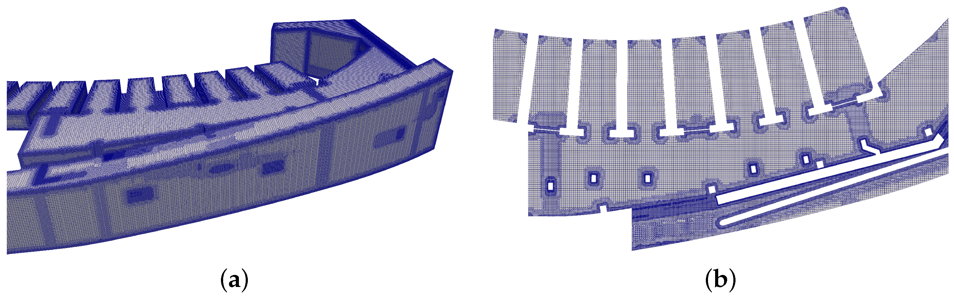
From the CAD model, different STL files were created, differentiating for each specific boundary patch and separating the walls into different types of geometries to increase the refinement control: small pipes, large pipes, ventilation ducts, and small details. The mesh was generated using OpenFOAM’s meshing tool SnappyHexMesh, with an initial cell size of 10 cm. Then, different surface refinement levels were defined, along with specific volumetric refinement zones to reproduce all the details of the room. The smaller cell size corresponding to the region near the ventilation grilles and other geometric details is $6.25$ mm. The total area represented by walls in the system is $2282{\mathrm{m}}^2$; considering the number of cells required to properly resolve the wall boundary layer for the total wall surface by means of an appropriate inflation, it is clear that the computational resources required would make impractical the creation of the desired dataset of simulations. Having this limitation in mind, no inflation layers were included, expecting to encounter low velocity gradients near the walls. Thus, the wall boundary layer was modeled relying on the use of wall functions that are well known and widely used in many research works using a RANS approach ($k-\epsilon$ model). This configuration yielded a mesh with 7.9 million cells. In Figure 3, some mesh details are shown, with a 3D image of the upper zone and a 2D slice at 4.55 m from the ground.

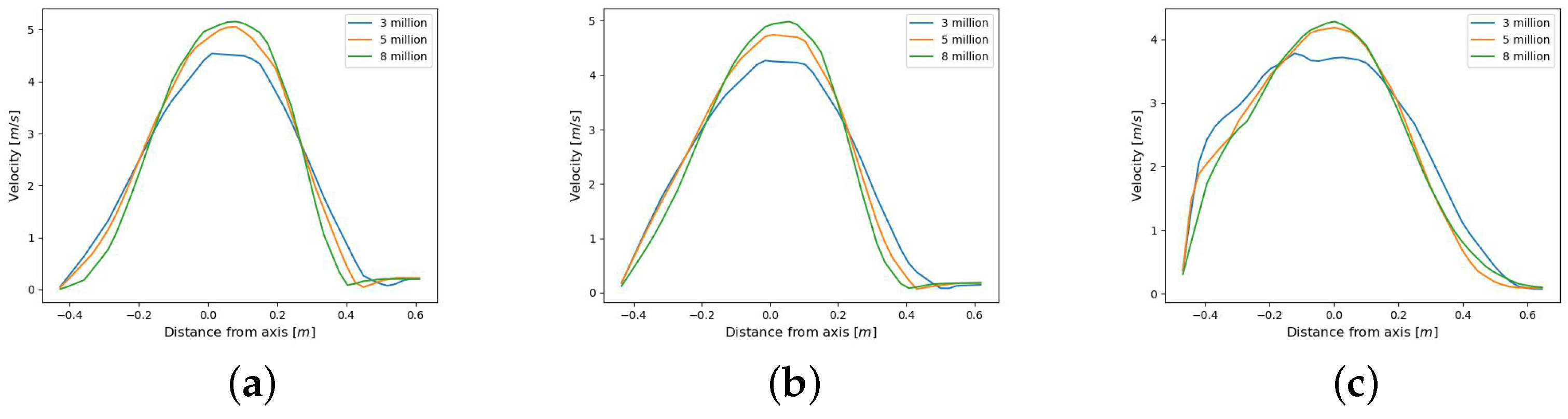
Additionally, a mesh test was performed to assess its effect on CFD convergence. To this end, two more meshes were evaluated, comprising 5 and 12 million cells. A case with maximum ventilation flow was used to compare the effect of the mesh. The converged velocity profiles were obtained at different distances from the supply grill. Figure 4 depicts the three profiles at different distances for each mesh, showing that the obtained velocities converge towards the 12 million cell mesh. A noticeable difference is present between meshes with 5 and 8 million cells, although velocity profiles converge towards the finest mesh. The results indicate that the intermediate mesh used in this study (7.9 million cells) can be regarded as sufficiently refined to yield good results to train a predictive model, optimizing the computational cost of creating the dataset.

After the mesh is generated, the boundary conditions need to be defined for the different patches of the domain. Each special patch has been introduced in Figure 1, and then variables with special treatment associated with these patches have been listed in Section 2.3. The summary of the complete configuration for the main types of boundaries is presented in Table 2. Relative humidity and temperature of the supply circuit were set accordingly with the typical psychrometric conditions of each corresponding season from data extracted from a weather station located near the Oceanogràfic. The ranges for both variables are temperature $=[280,308]$ K and relative humidity $=[30,85]\%$, considering days and nights within the whole year, excluding extreme conditions outside the typical ranges of each season. The relative humidity at the exhaust grilles of the drying circuit was set at the operating point of the machine (60%), although lower values below 30% were considered for a subset of the dataset. The temperature of the water surface was kept constant to 293 K for the complete dataset. This configuration is justified because the water from the aquarium was kept at constant conditions by the machinery present in the technical room due to the biological requirements of the marine fauna present in the aquarium. Finally, the psychrometric conditions of the swap surface were chosen among a defined range obtained from the study of the typical values of temperature and relative humidity of the gallery at different times of the year. The ranges for both variables are temperature $=[288,297]$ K and relative humidity $=[55,87]\%$.

Since the goal of the simulations is to obtain the final equilibrium state of the room for a given set of psychrometric variables and actuators settings, steady-state simulations were performed until reaching convergence. To this end, the temporal derivative was not considered in any equation—as shown in Equations (2), (3), and (5)—and thus, there was no need to adjust the time step to ensure a Courant number smaller than 1. Second-order advective schemes were selected for the majority of the variables, excluding the turbulent variables -k and $\epsilon$-, where first order was used to ensure its boundedness and provide stability to the simulation. The convergence criteria used were $1\times {10}^{-3}$ for the pressure and $1\times {10}^{-4}$ for the velocity, temperature, and specific humidity.

Employing the previously described CFD models and boundary conditions configured accordingly with the defined set of cases (https://zenodo.org/records/15025264, accessed on 14 March 2025), the complete dataset was generated.

2.5. AI Model

2.5.1. Data Preprocess for Training

As explained in Section 2.3, the obtained dataset was composed of 142 CFD cases, and each case was defined by a set of 15 variables (related to initial conditions, boundary conditions, and actuators) that served as inputs to the CFD–AI surrogate model. Then, to train the predictive model to infer the equilibrium state of the whole domain, the resulting 3D fields of temperature and relative humidity were extracted from the CFD simulations.

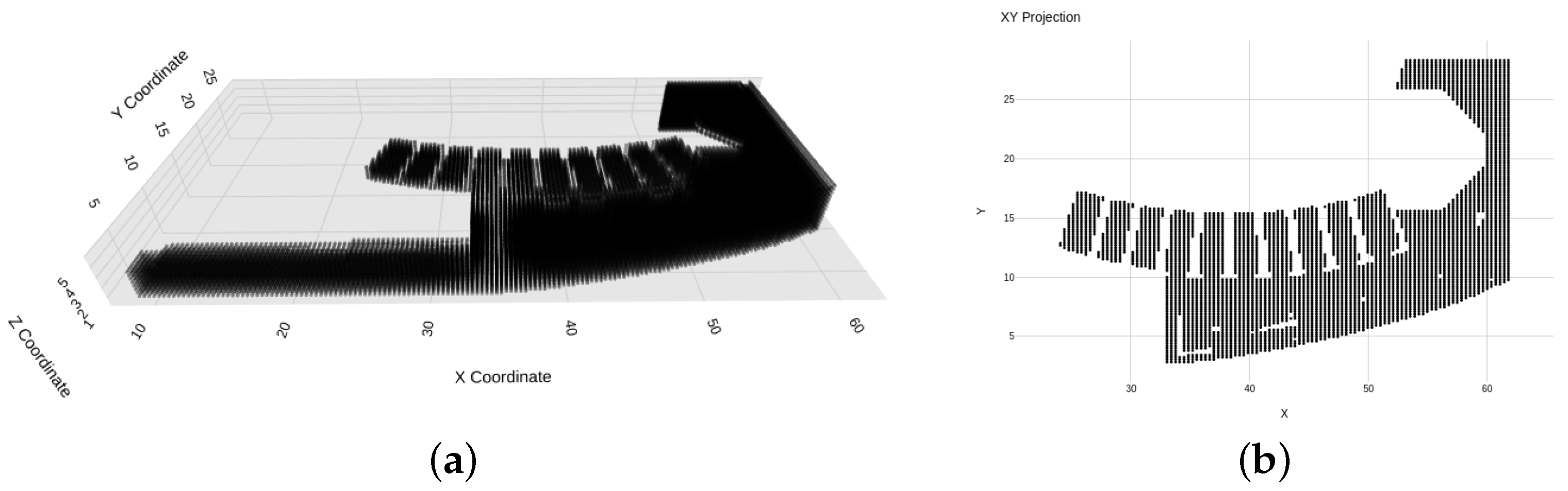
Due to the immense amount of cell data and its non-uniform spatial distribution, a secondary grid was constructed, featuring points uniformly distributed. The points were arranged aligned with the main axis of the domain, separated from each other by 35 cm. The extracted temperature and relative humidity values were sampled by linearly interpolating the data of the surrounding cell centers of the primary mesh. This sampling grid resulted in roughly 62,000 points for each predicted variable, yielding a total of 124,000 output points. In Figure 5, the 3D spatial distribution of the sampling points is shown, along with a 2D horizontal slice, showing that the sampling grid adapts to the domain shape and internal cavities of the primary mesh.

Thus, the CFD data used to train the CFD–AI surrogate model can be summarized in the following: 15 input data comprising boundary conditions, actuator flow rates, and 3 virtual sensors inside the domain; and 124,000 output data from the 3D fields interpolated to the regular mesh shown in Figure 5, comprising temperature and relative humidity data.

2.5.2. Model Architecture

To construct the surrogate model, a neural network (NN) based on the Multilayer Perceptron (MLP) architecture was employed. The MLP was characterized by its fully connected layers, meaning each neuron is connected to every neuron in the adjacent layers. This dense connectivity significantly increases the number of parameters in the neural networks, demanding substantial computational resources [38]. Despite this complexity, MLPs are widely used due to their versatility in various applications. Recent works can still be found where the use of MLP can deliver results up to the required standards. To this regard, the work of Mansour et al. [39] can be cited, where an MLP-based architecture is used for image reconstruction. Authors find that this architecture enables image reconstruction performance slightly better than a U-Net NN. Similarly, Albasiouny et al. [40] used an MLP-based architecture for a generative model, finding that this model proved to be more efficient and robust than a model solely based on convolutions. These works encouraged the use of the present architecture to tackle the problem given in this work.

The key complexity of this work is the high ratio between the number of inputs and outputs (15 to 124,000). MLPs have proven to be a suitable architecture when such a high generation of data is needed. Another complexity arises from the low amount of training data; as explained in Section 2.3, this comes from a limitation in the possible combination of psychrometric variables, which leads to low batch sizes and low cases available for training. As a precedent work, Liu et al. [41] employed deep NN based on MLP for high dimensionality data with low sample size with satisfactory results, which also supports the present selection of NN architecture. Furthermore, more sophisticated NN like convolution-based or graph-based were not tested, as the low amount of training data was expected to be insufficient to properly train such models.

It should be noted that, in this work, simpler ML models like Decision Trees, Random Forests, or Support Vector Machines were not tested. This decision was based on the large number of outputs, as these models are often used for tabular data and lower dimensional problems. However, some state-of-the-art works remark the capability of models like XGBoost to handle these types of problems and should be explored in the future [42].

To prevent overfitting —a common issue where the model performs well on training data but poorly on unseen data— dropout layers were included. Dropout is a regularization technique where a fraction of the neurons is randomly set to zero during training, preventing the network from becoming too reliant on specific neurons and promoting generalization. The total dataset was split into $80\%$ of cases for training the predictive model and the remaining $20\%$ was used to validate the accuracy of the model. All the accuracy results shown in the Results section are extracted using the validating subset.

When it comes to architecture definition and training hyperparameters, several degrees of freedom must be considered for this problem. These parameters include number of hidden layers, number of neurons per layer, dropout rates, and learning rate. In order to optimize the CFD–AI surrogate model to its maximum accuracy, a framework for hyperparameter optimization (Optuna) was used. Optuna [43] uses an efficient sampling algorithm to explore the parameter space, balancing exploration and exploitation to find the best possible solution. It supports various optimization strategies, including Bayesian optimization, grid search, and random search, making it highly versatile for a wide range of applications. A generalized scheme of the optimization algorithm is depicted in Algorithm 1, which serves to illustrate the optimization workflow. There, the studied parameters in line 3 can be number of layers, number of nodes, etc.

Algorithm 1 Optimization process with Optuna.

1: Initialize Optuna study with direction=’minimize’   2: for each trial in study do   3:    Suggest value for the studied variables   4:    Set data and architecture based on suggested values   5:    Train model   6:    Predict temperature and humidity fields using the trained model   7:    Evaluate loss based on the predicted fields compared to CFD data   8:    Return loss as the objective metric   9: end for 10: Optuna → minimize objective metric 11: Retrieve best variable values

2.5.3. Optimization of Sensor Locations

After the architecture is refined, an additional source of variability remains, as the locations of the 3 sensors inside the technical room are not predefined and therefore can be located anywhere inside. These virtual sensors are responsible for conveying information about the present state of the room to the predictive model. As stated before, it is not possible to know a priori which locations are going to deliver more information to the predictive model and therefore yield better results. As a consequence, different sets of sensor locations need to be tested to obtain the best suitable combination.

Assuming independence between the different stages of the optimization process, the optimization was performed in a sequential manner. First, the optimal neural network architecture was determined, as previously described. Subsequently, a second optimization stage was carried out using the Optuna framework to identify the most suitable combination of sensor locations. In this stage, Optuna was employed following the procedure outlined in Algorithm 1, where the parameters under study were the indices corresponding to the potential input (sensor) locations. By treating the architecture selection and sensor placement as decoupled stages, this approach simplifies the overall optimization workflow while still enabling the identification of an effective configuration for the sensing system.

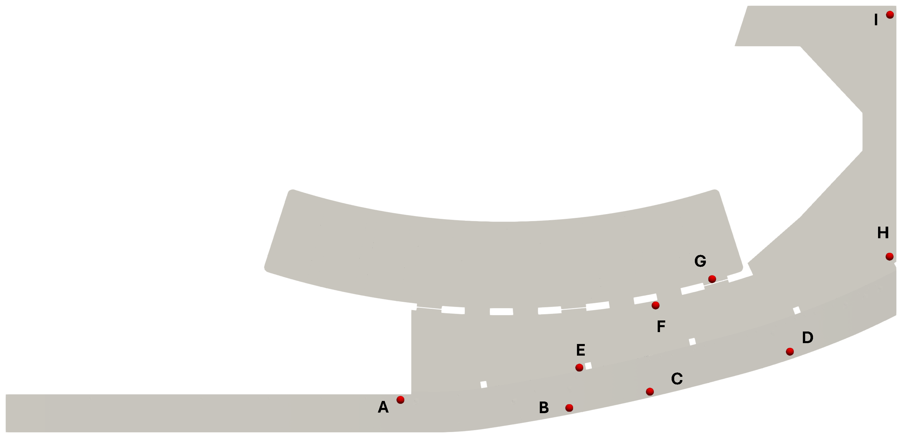
To carry out the described process, different sensor placements were defined from a preliminary study of the CFD simulations, identifying the most representative locations of the state of the room. From those locations, 50 different combinations of 3 sensors were defined, varying the X, Y, and Z coordinates. This process aimed to identify the optimal sensor configuration that would minimize the model’s loss function and enhance its predictive accuracy. In Figure 6, a schematic of all possible sensor placements is illustrated, including variations along the Z axis.

3. Results

In this section, the results for the different stages of the present work are shown. First, the obtained simulation results are investigated for a specific case to study the coherence of the converged solutions with the CFD models. Then, the outcomes of the optimizing process are shown, indicating the final architecture and training configuration, as well as the selected points for the virtual sensors that will provide input data to the predictive model. Finally, the accuracy of the model is investigated, showing an example case from the validation subset and computing the overall predictive error for the temperature and relative humidity.

3.1. Simulation Results

In this subsection, a case from the training dataset will be analyzed to illustrate the interaction between the different elements and ventilation circuits in the room. To demonstrate the effect of the supply and dryer circuits, a case with maximum ventilation flow and typical temperature and humidity is studied, with the configuration detailed in

Table 3. Simulation case configuration.

Variables	Values
Supply flow (m3/h)	3000
Exhaust flow (m3/h)	3000
Drying flow (m3/h)	3000
Initial room temperature (K)	294
Swap temperature (K)	294
Dried air temperature (K)	299
Supply temperature (K)	292
Wall temperature (K)	292
Initial room relative humidity (%)	85
Swap relative humidity (%)	82
Dried air relative humidity (%)	60
Supply relative humidity (%)	55

.

The converged results of the simulations can be seen in Figure 7. The streamlines in Figure 7a represent the air currents from the discharge grilles of the drying circuit. The relative humidity ranges from 60% at the grills to almost 100% in the interior of the chamber, showing that the dried air entered the chamber and slightly reduced the relative humidity in the interior of the cavity. This validates the design idea of using the dehumidifier system to directly lower the moisture content inside the chamber, especially the ceilings, where the majority of the water condensation occurs. Following a similar philosophy, the grilles of the exhaust circuit are located inside the chamber (as shown in Figure 1), in order to extract the air with the greatest humidity content outside of the facility.

Figure 7b represents a set of streamlines starting from the supply discharge grille, also colored according to the relative humidity. Here, the fresh air is directed towards the drying intakes and reaches the least renovated zones of the technical room (left side in the picture), providing fresh air and helping homogenize the temperature and humidity of the whole facility. As the supply circuit is untreated air from the exterior, depending on the external psychrometric conditions, the introduced air will constitute a source of additional humidity to the system or will dilute its concentration. For this case, the air injected also has a low content of water vapor, increasing its concentration as it mixes with the air inside the room.

Although it is not represented, from Table 3, it can be seen that the flow rate of pumped air for the supply and exhaust circuits is the same. This net balance between the exhaust and supply circuit generates a low net flux between the room and the gallery, reducing the exchange of humidity to its minimum. This configuration can be used to isolate the technical room as much as possible from the gallery.

Finally, to better visualize the different distributions across the room, 2D slices at different heights plotting the velocity, temperature, and relative humidity are shown and analyzed in Appendix A.1 for the presented case.

3.2. Architecture Optimization

As explained in Section 2.5.2, the model’s architecture was optimized using Algorithm 1 with a set of pre-selected sensor locations. The final architecture obtained is depicted in Figure 8, comprising three dense layers followed by dropout layers.The configuration regarding the training hyperparameters is detailed in

Table 4. Hyperparameter configuration of the optimized surrogate model.

Hyperparameter	Configuration
Optimizer	Adam
Learning Rate	$4.69\times {10}^{-4}$
Loss Function	Huber
Training Iterations	1000
Number of Batches	4
Dropout Rate	0.456

. The Huber loss [44] was used as loss function to train the model. The reason for this choice is that it is used for weather forecasting [45], and according to Borah et al. [46], it provides a better generalization with lesser sensitivity towards noise and outliers, which matches the requirements for the present work.

3.3. Sensor Location Optimization

Regarding the second stage of the optimizing process, sensor locations where selected to optimize the input information to the surrogate model regarding the state of the room. This allowed us to fix the degrees of freedom regarding this aspect and maximize the predictive performance of the model. After applying the same algorithm to different sets of sensor locations, the optimal positions obtained are detailed in

Table 5. Optimal sensor positions.

Sensor	Coordinate X	Coordinate Y	Coordinate Z	Scheme Position
0	61.7	27.0	1.75	I
1	61.7	14.0	1.75	H
2	43.5	4.25	2.80	B
3	43.5	4.25	4.55	B

. In all the different combinations, three sensors were swapped between locations, while one sensor remained fixed near the swap surface to monitor the air exchange with the gallery. Note that two sensors share the same X and Y coordinates, but are located at different heights: one at the same height as the supply grille, and the other at the same height as the dehumidifier system, meaning that the neural network understands the relation between those circuits and the equilibrium state of the room.

3.4. Model Accuracy and Validation

After determining the optimal sensor positions, the final version of the surrogate model was trained and its predictive capability was validated against CFD simulation results. To quantitatively evaluate the predictions of the CFD–AI surrogate model, two main metrics were used: Mean Absolute Error and Mean Relative Error, computed for both the relative humidity ([%]) and temperature ([K]) according to the following equations:

$$MAE={\displaystyle \frac{1}{N_C}}{\displaystyle \frac{1}{N_P}}\sum _{i=1}^C\sum _{j=1}^P\left|\right(y_{i,j}-y_{i,j}^{\prime }\left)\right|$$

(6)

and

$$MRE[\%]={\displaystyle \frac{1}{N_C}}{\displaystyle \frac{1}{N_P}}\sum _{i=1}^C\sum _{j=1}^P{\displaystyle \frac{\left|\right(y_{i,j}-y_{i,j}^{\prime }\left)\right|}{y_{i,j}}}100$$

(7)

with C being the number of cases in the validation subset, P the number of predicted points at each case, $y_{i,j}$ the ground truth value of the ith case at the jth point, and $y_{i,j}^{\prime }$ the predicted value. Using these metrics, the overall MAE obtained for the validating subset yielded an average error of 0.34 Kelvin for the temperature and 2.2 percentage points for the relative humidity. Translating these absolute errors to relative by computing the MRE, this yields a corresponding $0.11\%$ for the temperature and a $2.3\%$ for the relative humidity.

To illustrate the overall spatial accuracy of the CFD–AI surrogate model, the complete predicted data from a case with average MRE was compared with its ground truth. As the predictive model is trained using the extracted data from the point grid shown in Figure 5, the outputs of the model correspond also to the temperature and relative humidity to that sampling grid but unordered. Consequently, in Figure 9, the predictions from the selected case are presented in a scatter plot, without any spatial ordering, for temperature (a) and relative humidity (b). Different levels of relative error (red) have been defined to help the reader visualize the general error committed by the predictive model for this case. Also, a linear regression was adjusted between predicted and ground truth values (green), also indicating the fitted coefficients for each regression and the coefficient of determination ($R^2$). It can be observed that the majority of the points predicted present a low deviation from the ground truth, with errors typically around 2.5%, although zones with higher errors can also be found up to 5%. This indicates that the majority of the predicted domain displays an acceptable level of error with respect to the ground truth values. Although the slope coefficients of the linear regressions show room for improvement, they indicate that the model is able to identify which ventilation circuits are active and what is the result of the specific weather conditions of that day, providing a good tendency of the approximate evolution that the system is going to have.

In addition, by knowing the coordinates of each point comprising the point grid, the predictions can be re-arranged into their original 3D location. In Figure 10, the predicted relative humidity for the same case is shown at four different slices as an example of how the data generated by the CFD–AI surrogate model can be relocated spatially. Here, clips of the original domain can also be performed to isolate specific areas of interest. The capability of recovering the spatial information is key for the future implementation of this predictive model in a digital twin core. This will allow us to define complex control rules and evaluation metrics for the state of the room. As an example, in Figure 11, two specific filters have been applied to the predicted values, showing all the points that have a temperature higher than $20 °$C (a) and those that also have a relative humidity higher than 88 [%] (b). The implementation of such kinds of conditional thresholds will allow the investigation of critical areas inside the domain and have a more specific control of key regions of the room.

To better illustrate the forecasting capabilities of the predictive model, inferences carried out by the predictive model for the example case have been re-arranged and displayed in Appendix A.2. The predictions are displayed in horizontal slices at 2.8 m and 4.55 m, selected as they contain the greatest variations in temperature and humidity. Predictions are accompanied by ground truth and relative error slices. A visual inspection of them reveals a strong agreement achieved by the predictive model.

4. Discussion

CFD simulations allowed us to gain insight on the dynamics of the system and how each ventilation circuit affected it. As observed, the net flow rate between supply and exhaust circuits allows us to control the exchanged flux between the technical room and the gallery: suctioning or pumping air from or to the gallery, or isolating the room. It is thus important to consider for the ventilation strategy the amount of air from the gallery that might enter the room and check if its temperature and relative humidity are beneficial or not.

Complementing these circuits, the drying circuit can effectively control and reduce high humidity in critical regions as the interior chamber. This circuit can act as an auxiliary tool to help control excessive humidity in a localized zone without the need of using high flow rates to have several renovations of air per hour.

The implemented evaporation/condensation model yielded coherent results, similar to [10,11,12,13], showing an accumulation of relative humidity inside the chamber due to the presence of the water surface. It also allows for the identification of the walls that present more condensation of water vapor, which in the future can be used by the control algorithm to evaluate the humidity content near these zones and act to prevent condensation.

It is important for the control algorithm to forecast the effect of the supply circuit in the system as a function of the amount of injected flow and its psychrometric conditions. When the external air has a low amount of water vapor, it will be beneficial to pump air in (e.g., in summer), whereas if the content of vapor is high (winter), the supply circuit will add extra humidity inside the room, increasing drying requirements and power consumption.

The explored methodology intends to use a surrogate model based on CFD simulations to provide a steady-state 3D distribution of temperature and relative humidity of the room. This ML tool can serve to implement a predictive control based on a digital twin.

Based on the insight gained with the CFD simulations, the set of variables that determine the configuration of the room climate were selected: initial conditions, supply and drying characteristics, and actuator flow rate. A total of 15 variables were chosen: 8 for the determination of initial conditions, 4 for the supply and drying, and 3 for the actuators.

To develop the surrogate model, an analysis of real psychrometric data was acquired over one year. This analysis served to develop a set of CFD simulations comprising conditions that are representative of the true behavior of the room during the year. The CFD dataset encompassed maximum, minimum, and medium conditions for each season so that the surrogate model could effectively handle realistic environmental variations. By incorporating the effects of water evaporation on the water surface and water condensation on walls and equipment, the CFD simulations were able to reproduce the expected behavior of the room and the impact of the different ventilation circuits on the psychrometric equilibrium state.

A total of 142 cases were generated from the defined combinations described, which comprised the dataset used to train the surrogate model. The chosen architecture—an MLP—was enhanced with dense layers and dropout layers to mitigate overfitting. The architecture was optimized in two stages. The first stage served to tune the training hyperparameters and model size using the Optuna framework, resulting in an efficient configuration that performs predictions in milliseconds, as opposed to the hours required by the CFD simulations.

The second stage aimed at optimizing the locations of the sensors determining the initial conditions. This secondary optimization improved the accuracy of the surrogate model, and also identified locations in close relation with the ventilation circuits. The selected points prove that the CFD–AI surrogate model is effectively learning the physical interaction between the ventilation circuits and the psychrometric state of the room.

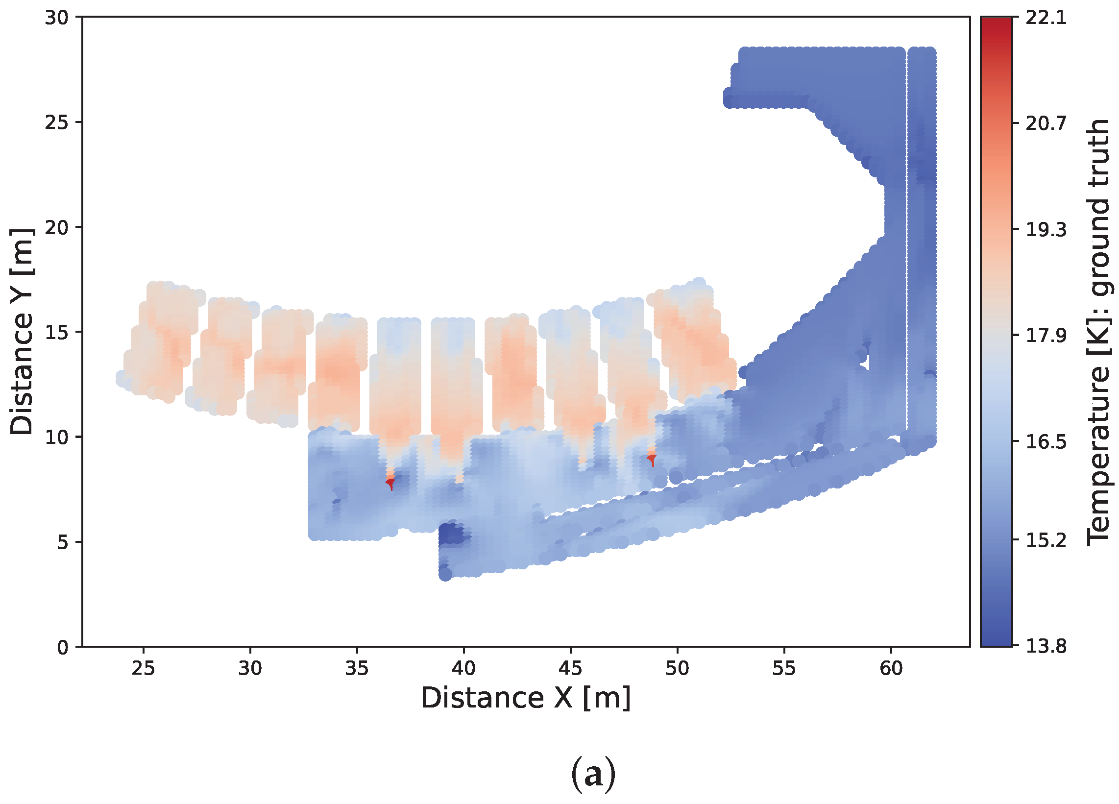
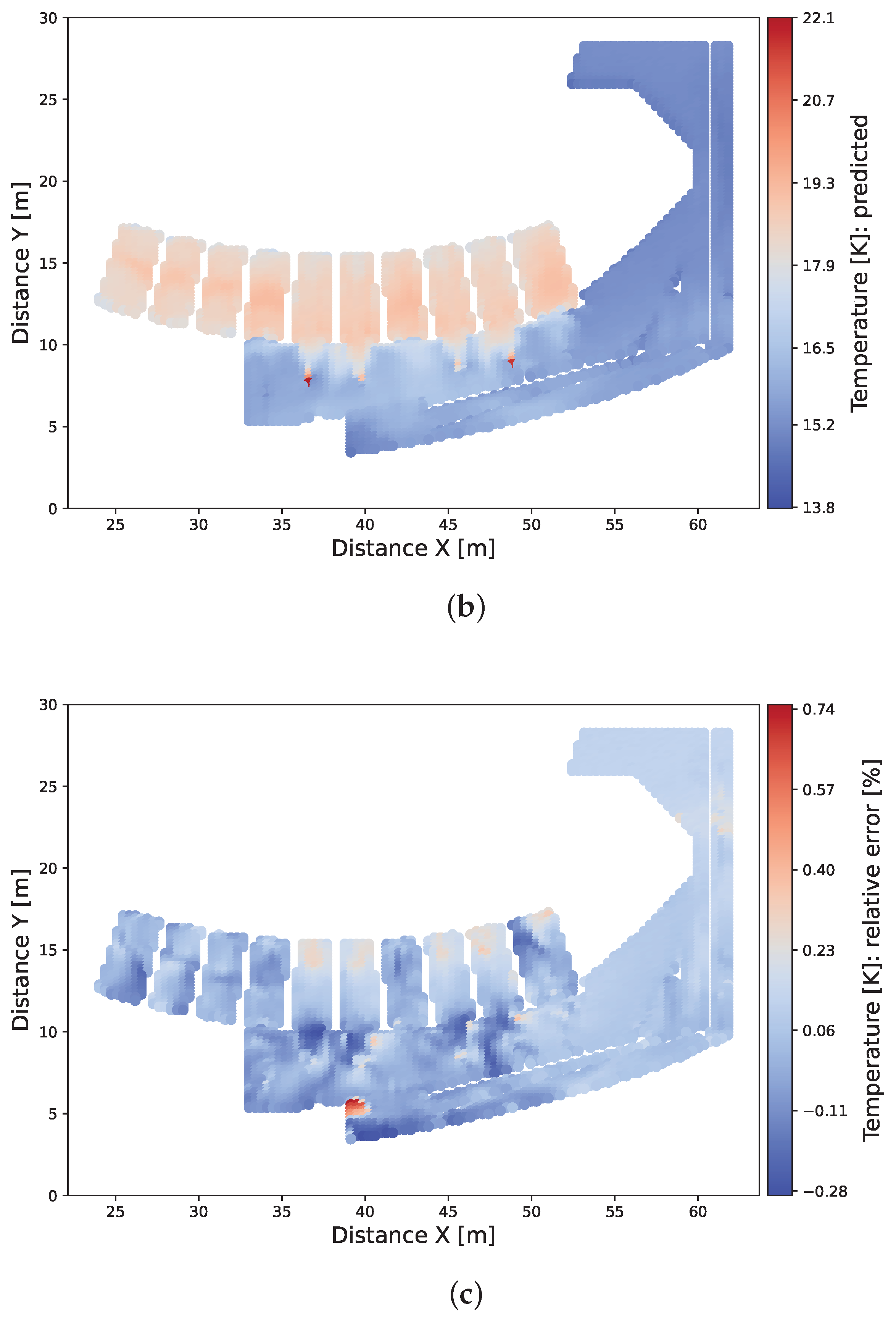
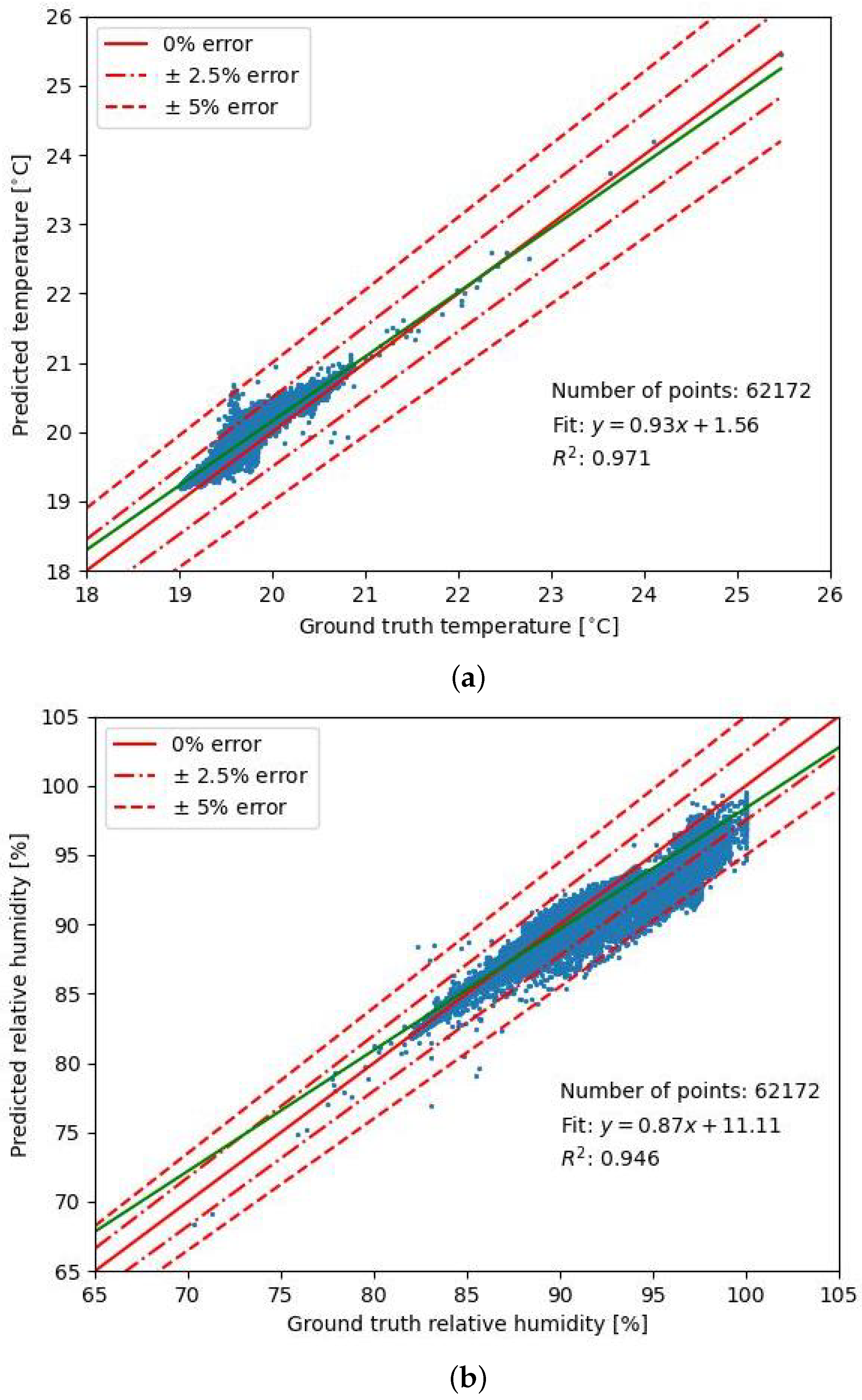
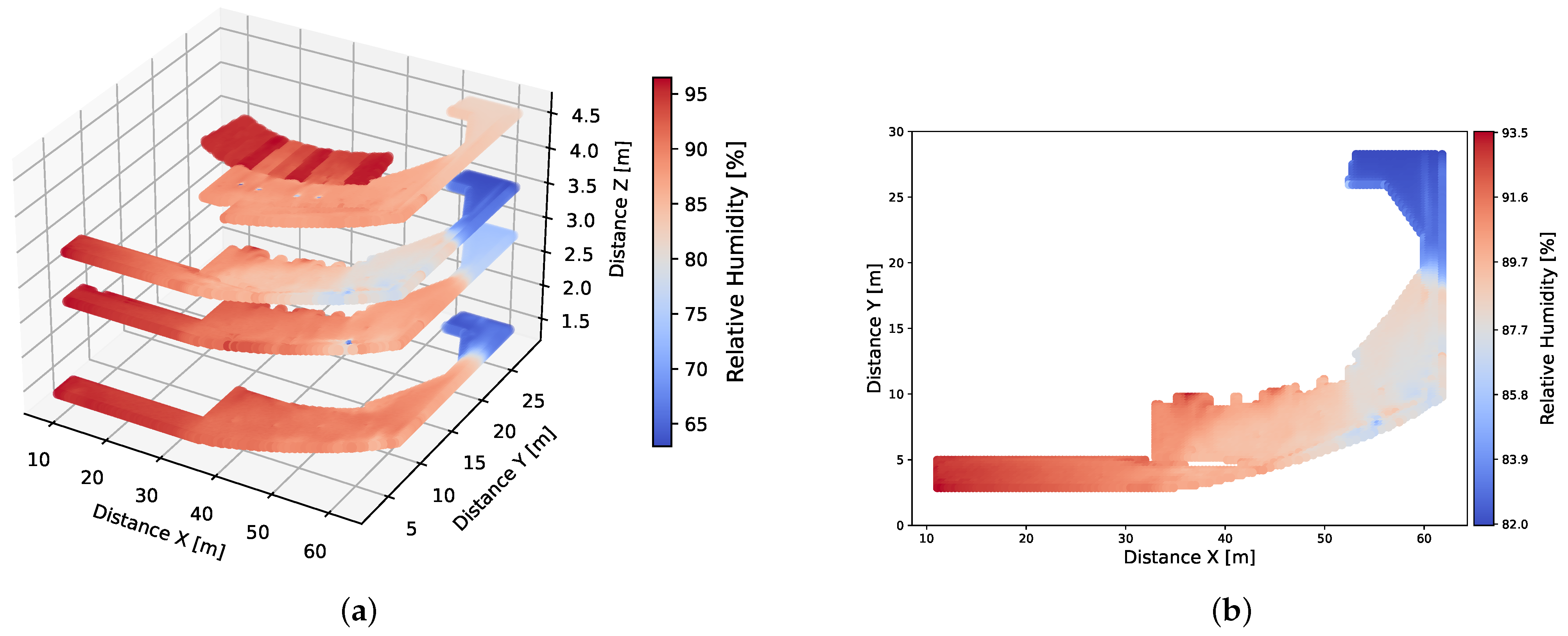
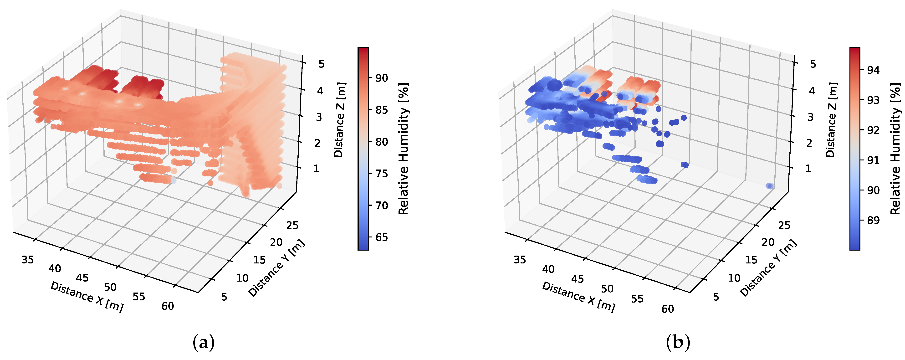
The resulting surrogate model was capable of delivering predictions with average errors of 0.34 degrees Kelvin for the temperature and 2.2 percentage points for the relative humidity. The capability of recovering the spatial location of the inferred points helped in comparing the model’s predictions with the CFD results. Upon these comparisons, the predicted model showed its ability to reproduce the general trends of the system, detecting the effect of the ventilation grilles and showing overall low relative errors. Thus, the spatial distribution of the temperature and relative humidity at general equilibrium state were satisfactorily predicted. Finally, two examples of possible filtering options for the predicted data were shown, demonstrating that the generated fields can be used for a more accurate spatial analysis of the system, allowing for more refined control strategies in the future. As the control strategy for a ventilation system will take into account different zones of the domain, the presence of regions with higher error will be dampened after averaging around several points. Thus, the obtained average errors can be considered sufficiently small to help on the control decisions by presenting the approximated evolution of the room.

The architecture used to create this surrogate model has demonstrated to be capable of learning to predict spatial distributions with high amounts of data from a reduced number of inputs. This demonstrates its versatility, in line with recent works conducted [39,40,41]. The presented results demonstrate the potential of surrogate models in flow prediction, allowing its future implementation in ventilation control to ensure optimal performance.

5. Conclusions

This paper demonstrated the feasibility of a new methodology to create a predictive model envisioned to be implemented on a digital twin for an unsupervised ventilation control. This predictive model is based on the developed surrogate model that combines data from CFD simulations and sensors. To demonstrate the methodology, CFD simulations of an underground technical facility have been performed, including the modeling of the relative humidity by implementing the evaporation and condensation of water vapor.

The training dataset was created to emulate the behavior of the actual system against different weather conditions and ventilation control points. An ML model was trained with this dataset to obtain a CFD–AI surrogate model capable of predicting the temperature and relative humidity distribution with low average errors—0.34 degrees Kelvin for the temperature and 2.2 percentage points for the relative humidity—by implicitly learning from the physical phenomena involved in the system. Each prediction was generated within approximately 131 ms, which is almost five orders of magnitude faster than the conventional CFD simulations used to train the model.

This work shows that it is possible to train such a predictive model to obtain inferences with high amounts of points from low sample data provided by sensors. This model takes the advantage of learning from smooth fields highly dependent on the ventilation circuits. Thus, the real dimensionality of the problem is reduced, as the predictive learns the general averaged spatial distribution and then applies specific changes accordingly with the inputs provided. More sensors can be included in the future to provide a better description of the system, generating more accurate simulations and supplying the predictive model with more information.

In the context of large ventilated rooms, this methodology opens the possibility for the implementation of such predictive models in control systems. Thus, a more detailed predictive control can be developed by having much more spatial information than with a reduced number of sensors.

Future work will focus on the real-time control of the room over short durations to validate and analyze the behavior of the digital twin. This will involve real-world implementation of the surrogate model to control the room’s ventilation system and collecting empirical data to compare against the model’s predictions. Based on these observations, the dataset will be expanded and refined to enhance the accuracy and reliability of the surrogate model and the implemented control.

This work will also be extended to more complex systems, moving beyond a single room to interconnected rooms or spaces with more complex geometries and larger domains. By scaling the approach, we aim to explore the digital twin’s capabilities in managing ventilation in more sophisticated and dynamic environments.