Abstract
This study proposes a three-dimensional numerical wave tank (NWT) to calculate wave propagation and hydrodynamic forces based on the Navier–Stokes equation, using commercial Computational Fluid Dynamic (CFD) software ANSYS Fluent. The VOF Method is utilized to identify the free surface. The CFD model employed for generating waves in the NWT is initially verified using analytical theory to evaluate the accuracy of the results. In addition, the User-Defined Function (UDF) in ANSYS Fluent is implemented to ensure the model performs under the oscillatory conditions of the Submerged Horizontal Plate (SHP) Wave Energy Converter (WEC) device, which is localized at the center of the NWT. Finally, the influence of SHP oscillation on the device’s average efficiency was analyzed by comparing seven cases with different geometric configurations, considering both the oscillating and non-oscillating conditions of the SHP under the incidence of different waves. The results indicated that the geometric configuration and wave conditions of Case 4 achieved the best performance, reaching an average efficiency of 35.68%.
1. Introduction
The importance of renewable energy is increasingly recognized as society becomes more aware of environmental challenges and the need to transition to more sustainable energy sources. As a result, various government institutes worldwide have undertaken initiatives and developed strategies to enable this transformation [1]. In addition, it is plausible to argue that the transition will not only promote the well-being of current societies, but it will also ensure the security and progress of future generations [2].
In this context, Brazil stands out due to its energy matrix, which is predominantly based on renewable sources. According to the Energy Research Company [3], the Brazilian electricity generation matrix, when compared to the global energy matrix and that of the member countries of the Organization for Economic Cooperation and Development (OCDE), presents a scenario with less environmental impact, with only 12.1% of national energy coming from non-renewable energy. On the other hand, the International Energy Agency (IEA) [2] highlights that both the global energy matrix and that of OECD countries have lower shares of renewable sources (Figure 1).
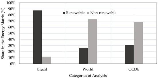
Figure 1.
Comparison of Brazilian and world energy sources.
According to the International Energy Agency [4], ocean energy is one of the most promising renewable resources, with a global potential of approximately 32 TW. Jusoh et al. [5] noticed that ocean waves can generate more than 100 kW/m of energy power density, a value higher than the intensity generated by solar and wind sources.
Brazil, with its extensive coastline of 10,900 km, has significant potential for wave energy exploitation [6,7]. Although its energy matrix is predominantly renewable, with a focus on hydropower, it is essential to diversify energy sources to reduce dependence on a single solution [3]. Rio Grande do Sul state, with 632 km of coastline and an estimated power of 38 kW/m [8], is a promising Brazilian region for the development of wave energy capture technologies, especially due to its location far from the Equator [9].
The current technologies for harnessing wave energy exhibit remarkable diversity, varying according to distinct energy conversion principles [10]. Among the technological alternatives, notable examples include devices based on body oscillation, point absorbers, attenuator systems, oscillating water column devices, and overtopping mechanisms, each with specific characteristics regarding efficiency, technological complexity, and suitability for different maritime conditions [11].
Despite their significant potential, few wave energy converters (WECs) have reached the advanced stages of technological maturity, hindering their large-scale implementation. The Technology Readiness Level (TRL) system [12], widely used to assess technological progress, consists of nine levels, from TRL 1 (initial concept) to TRL 9 (full operational implementation). Currently, most WECs remain at intermediate TRL levels (TRL 4 and TRL 5), meaning they have been validated in laboratory environments and demonstrated in controlled scenarios but have yet to undergo extensive real-world testing.
Among the various wave energy technologies, the Submerged Horizontal Plate (SHP) WEC is one alternative [10,13], a device that converts the kinetic and potential energy of waves into usable energy. The SHP consists of a submerged plate positioned parallel to the mean sea surface and anchored to the seabed. As waves pass over the plate, they generate an alternating water flow beneath the structure. This flow can be used to drive a turbine installed below the SHP, converting wave energy into electrical energy (Figure 2).
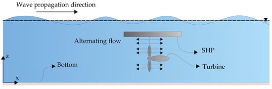
Figure 2.
Illustration of the SHP system.
These structures operate in challenging environments characterized by waves, marine currents, and high-intensity winds. Consequently, waves play a crucial role and are one of the main parameters to be considered in the design of offshore structures [14].
The use of Computational Fluid Dynamics (CFDs) employed in this study is justified by its efficiency and flexibility in modeling complex wave–structure interactions [15], offering significantly lower costs compared to analytical and experimental methods. Although analytical methods are useful in simplified conditions [16], they have limitations in solving three-dimensional and nonlinear problems due to the complexity of the involved equations. On the other hand, physical experiments require high financial investments, large physical space, and considerable execution time [14,17]. CFD, on the other hand, allows detailed simulations in various scenarios, making it the most suitable alternative for the objectives of this study.
Thus, initially, a 3D numerical tank is modeled with the same dimensions as those used in the studies of Orer and Ozdamar [18], Seibt et al. [13], and Goulart et al. [19], enabling validation and verification of the model based on previously consolidated results. After this step, the dimensions of the numerical tank were strategically increased to simulate waves with specific characteristics of the study area, ensuring that the results are robust and applicable to the problem at hand.
This approach seeks to maintain result quality while overcoming the limitations of physical tanks. In this context, with the progress in data processing, it becomes possible to use CFD codes for this purpose. To simulate linear waves and the nonlinear motions of floating structures in water, various numerical modeling approaches are employed, including the Boundary Element Method (BEM), the Finite Element Method (FEM), and the Finite Volume Method (FVM) [20].
Several researchers have contributed to the development of this area. Bihs et al. [21] created a 3D NWT to analyze the propagation of waves and calculate the associated forces, based on the Navier–Stokes equations. Tutar and Mendi [22] analyzed turbine performance through a wave volume analysis, utilizing the Volume of Fluid (VOF) method combined with the FVM. Additionally, Tang et al. [23] studied the dynamic characteristics of a double pontoon floating structure, applying a fully nonlinear 2D NWT, where the BEM method was applied to calculate wave loads.
Dong et al. [24] conducted experimental investigations to analyze the forces generated by monochromatic and solitary waves on a horizontal submerged plate (SHP), using a wave channel in a laboratory setting. The study examined in detail the variation of wave forces under different channel bed configurations (flat or inclined) and evaluated how these changes influence the stability and performance of the device. The results indicated that, for regular waves, the forces on the SHPs increase proportionally to the relative wavelength until reaching a plateau, with nonlinear effects, such as wave deformation, becoming dominant. In the case of solitary waves, it was found that the forces increase with wave height, with the submersion depth primarily affecting the vertical forces and pitching moments, while bed inclinations reduce certain force components.
Cummins et al. [25] investigated the interaction of regular waves with inclined plates emerging on the surface, highlighting the impact of resonance phenomena on the generation of large hydrodynamic forces on the plate. Using the boundary element method and computational fluid dynamics (CFDs), the study revealed that the plate’s inclination significantly influences the excitation forces acting on the structure. The key findings include the following: (i) the wave forces are predominantly determined by the wave height in the channel, except during resonance conditions, when the forces may approach zero; (ii) for small inclination angles, resonance has a greater influence on the wave height, while larger angles reduce this effect; and (iii) maximizing energy capture requires a cautious approach when applying linear potential flow theory for power predictions.
Seibt et al. [26] applied a constructal design to a full-scale numerical model of a SHP used as a wave energy converter (WEC), aiming to optimize the device geometry and enhance its efficiency in electricity generation. The study analyzed the device’s operational principle and demonstrated that geometric alterations significantly impact the oscillatory flow beneath the SHP. The highest axial velocity was achieved with a specific geometry, representing a substantial increase compared to the lowest observed result. Similarly, the mass flow rate varied widely, with the highest value being 19 times greater than the lowest. The optimized geometry provided a peak efficiency for the SHP, with a minimum improvement of 35% over the least efficient geometric configuration.
Motta et al. [27] evaluated the efficiency of an SHP under regular waves, considering different geometric configurations and inclination angles. The computational model used a full-scale regular wave channel, employing the volume of fluid (VOF) model to simulate the water–air interaction and the finite volume method (FVM) to solve the transport equations. The results indicated that the SHP’s efficiency varies according to its inclination, with the optimal case at θ = 15°, where efficiency improved by 11.95% and 16.59% for breakwater (BW) and WEC, respectively.
The mentioned studies focus predominantly on SHPs, without considering the oscillation of the submerged plate in the computational domain. This study uses Navier–Stokes equations to analyze the efficiency of SHP devices under oscillated (O) and non-oscillated (NO) conditions in a 3D NWT. The VOF model is employed to determine the free surface, while the FVM is applied to solve the transport equations of mass and momentum. In addition, a UDF (User Defined Function) is implemented to model the oscillated movement of the SHP, allowing for the analysis of its dynamic behavior (Appendix A).
In general, the numerical models used in developing WECs account for factors such as site characteristics, climate variations, and the dynamics of waves or currents. However, the existing studies using the VOF methodology do not consider the device’s fluctuations, making this study innovative. Accounting for these oscillations in the computational domain is essential to improve the accuracy of simulations and provide a more realistic assessment of the SHP WEC performance.
This research aims to improve a numerical model that considers the oscillations of the SHP device, proposed to be installed on the coast of the state of Rio Grande do Sul, Brazil, submerged at 1 m depth in a location with 10 m of total depth. This study analyzes the impacts of these oscillations on the energy efficiency of the device. By offering an efficient and low-cost alternative for testing new energy solutions, this study aligns with global efforts toward sustainable energy transitions.
2. Computational Modeling
The numerical simulation is performed using the ANSYS Workbench 2020 R2 software, which provides an integrated platform for geometric modeling, mesh generation, processing, and post-processing. This environment enables detailed and accurate analyses of complex physical phenomena.
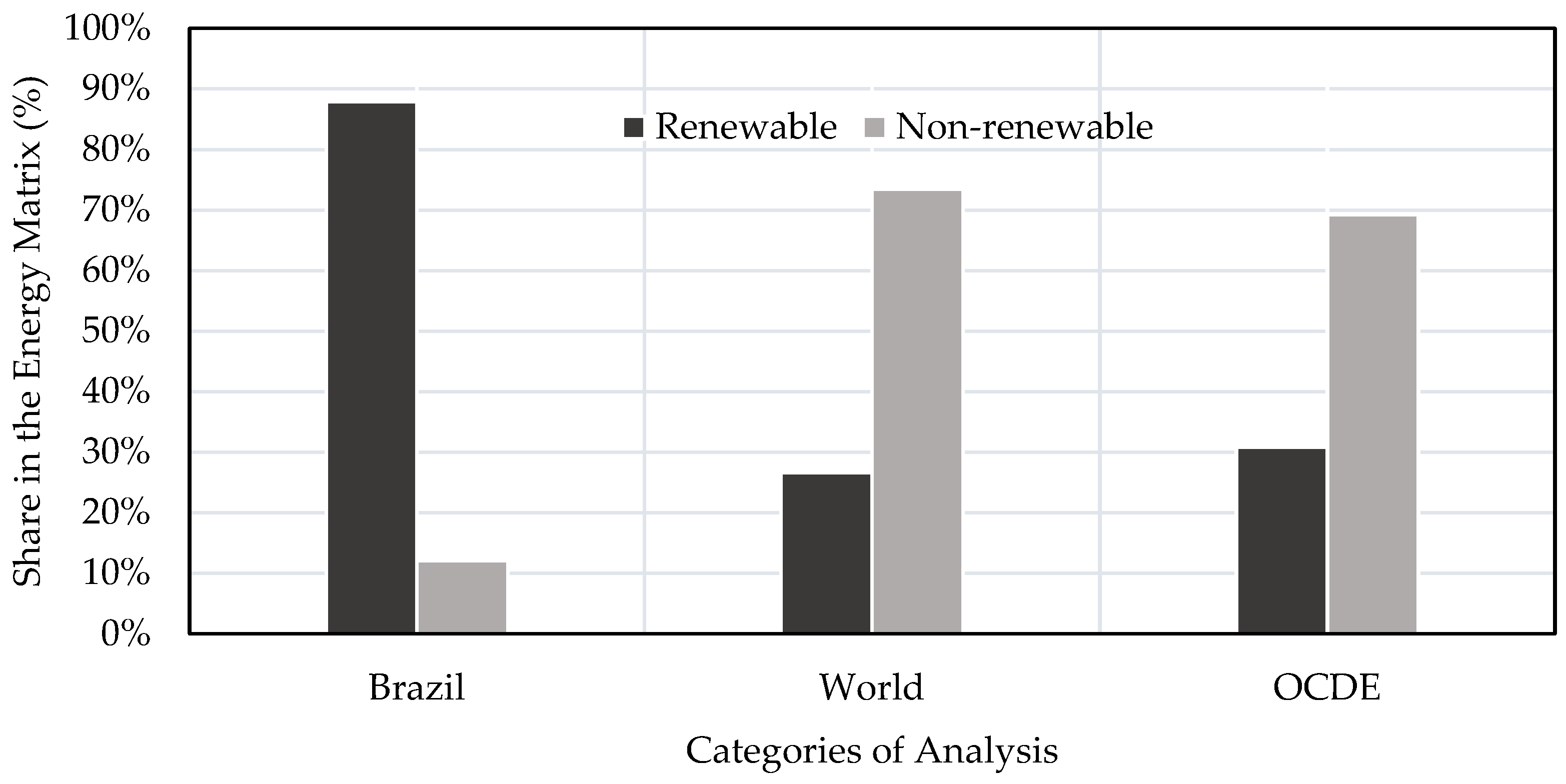
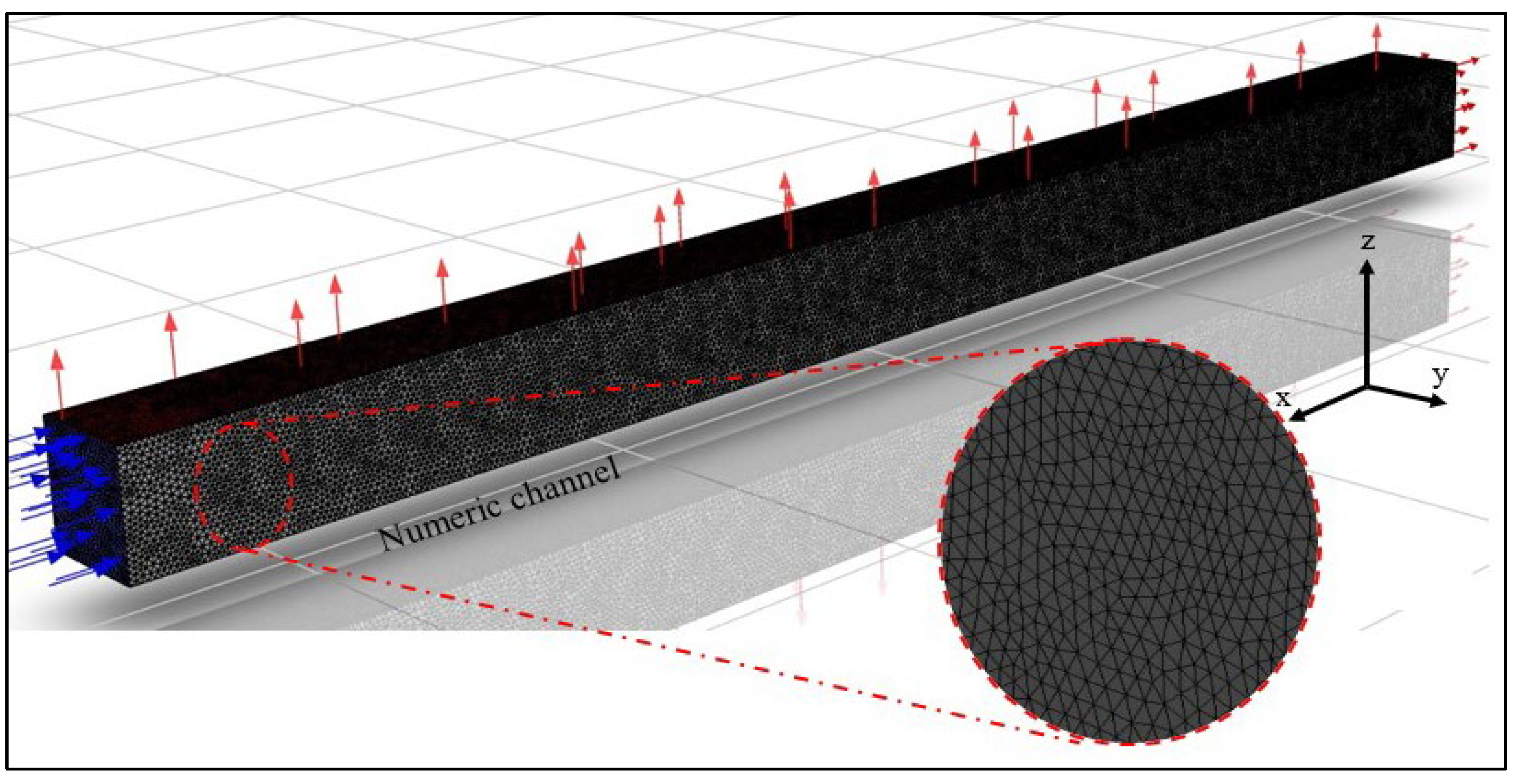
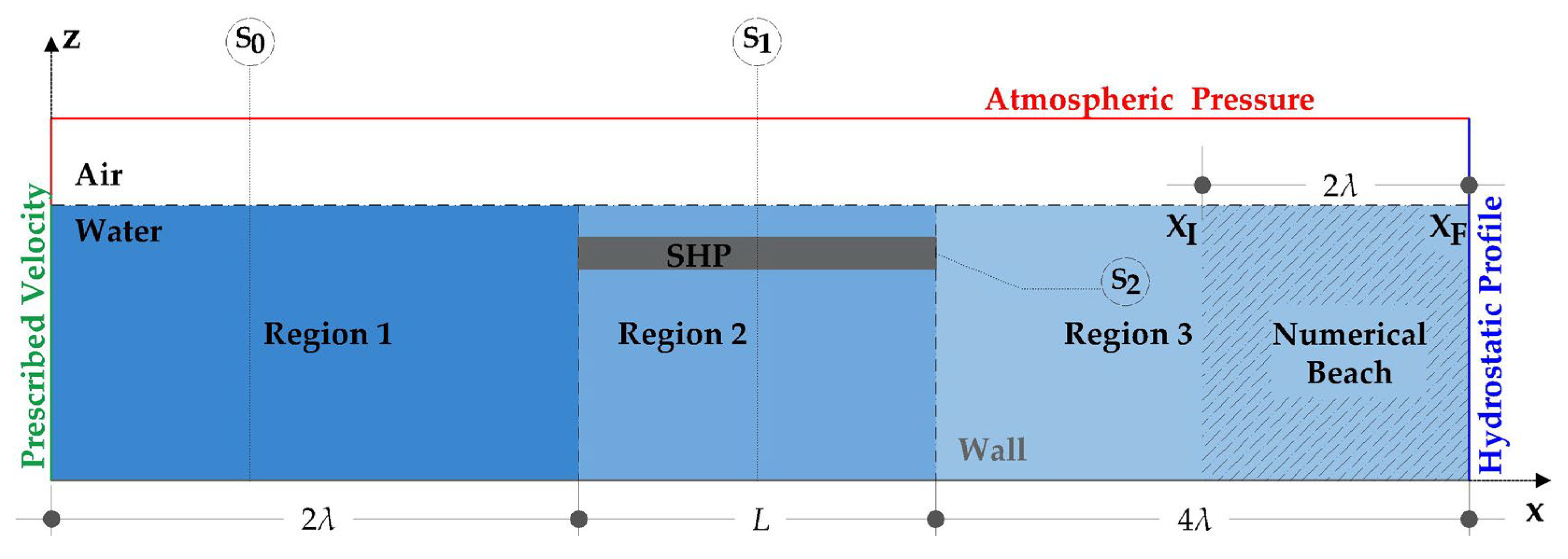
The computational domain in the numerical simulation includes a rigid SHP device, though displacements (z-axis) may occur due to its geometry. The SHP is positioned at the center of the three-dimensional wave channel, as illustrated in Figure 3. This channel has a length of = 327 m, a height of = 20 m, a width of = 20 m, and a depth of = 10 m (Figure 3A). Upstream of the SHP device is the wave propagation zone, which extends over two wavelengths (2λ). Next is the oscillation zone, with a length L. Downstream of the SHP, a distance of 4λ is maintained from its rear edge to the final wall of the wave channel, where the numerical beach is located, spanning 2λ [26], as shown in Figure 3A.

Figure 3.
Model Representation: (A) geometry parameters; and (B) boundary conditions.
The average characteristics of the ocean waves considered are a wave height H in the range 0.50 m ≤ H ≤ 1.50 m, a wavelength in the range 60.4 m ≤ λ ≤ 70.4 m, and a period of T = 7.5 s (Figure 3B). Thus, regular waves defined by second-order Stokes theory [28] are generated at the inlet boundary of the domain (green line—prescribed velocity) through the imposition of their two velocity components.
The second-order Stokes theory is chosen due to its ability to model nonlinear waves in typical shallow and deep-water conditions. Additionally, given the range of wave heights considered (0.5 m to 1.5 m) and the period of 7.5 s, which are typical of ocean waves in the area of interest [29], this theory provides a realistic approximation, capturing the nonlinear effects relevant to the analysis of wave interactions with the SHP device.
2.1. Volume of Fluid Model (VOF)
It is important to emphasize that the mathematical and numerical model used consider the flow as laminar, which simplifies the fluid’s actual behavior, as the transition between laminar and turbulent regimes is not clearly defined. The literature highlights the complexity of this phenomenon in the context of wave propagation in channels, where the precise delineation between these regimes is still debated [30,31,32]. Furthermore, the Reynolds number (Re) is widely used to characterize the transition between these regimes, but there is no universally accepted threshold, making it challenging to accurately model the fluid’s turbulent behavior [33].
Due to the interaction of these two immiscible phases, the VOF multiphase model is employed. Based on Hirt and Nichols [34], this model is suitable for systems with two or more fluids, ensuring that the volume of one phase cannot be occupied by the other phases [35,36]. The gravitational waves are governed by three fundamental principles: the conservation of mass, momentum, and the volume fraction, respectively, represented as follows [37]:
where ρ is the density (kg/m3), is the flow velocity vector (m/s), p is the pressure (N/m2), is the dynamic viscosity (Pa·s), is the strain rate tensor (N/m2), represents the volume fraction (dimensionless), and and are the buoyant forces and the external body forces, respectively (N/m3).
In this study, there are two phases considered: water and air, characterizing a two-phase flow. Cells with values between 0 and 1 represent the water–air interface, where . The ones that have are filled only with air (), while the others, are filled only with water ().
As mentioned above, a two-phase flow involves the average values of density and dynamic viscosity, which are calculated using the following equations, respectively [38]:
2.2. Boundary Conditions
In the simulation, the initial condition is set with the water in motion. Wave generation is achieved by the imposition of a prescribed velocity profile on the left side of the wave tank (green plane in Figure 3B), represented by the behavior of a wave generator [39]. Wave motion is generated by imposing the velocity field at the entrance of the wave tank; in other words, the velocity components along the x-axis and z-axis directions are the boundary conditions defined by the user [40].
The velocity components in the y-axis direction (transversal) are kept constant, with no variation along the x- and z-axes, indicating that the flow is essentially two-dimensional, focusing only on the x–z plane [40]. According to second-order Stokes theory, the movement in the y-axis direction (transversal) is considered negligible [13], implying the following:
Considering the second-order Stokes theory, the expressions that represent the horizontal u (m/s) and vertical w (m/s) components of the wave propagation velocity and the free surface elevation of the water (m) are given, respectively, as follows [28]:
where H is the wave height (m), k (m−1) is the wave number, h is the water depth (m), T is the wave period (s), (rad/s) is the frequency, and t is the time (s).
On the left side of the upper region and the upper surface of the wave channel (red planes in Figure 3B), the atmospheric pressure is set to Pabs = 101.3 kPa. At the bottom, right, and left surfaces, as well as at the surfaces of the SHP device (gray planes in Figure 3B), non-slip and impermeability conditions are imposed (u = w = 0 m/s). In turn, at the channel outlet, a hydrostatic profile is considered, where the water height is assumed to be equal to the depth of the NWT.
The submerged horizontal plate (SHP) movement in the x- and y- axes directions is restricted by the boundary conditions, allowing its movement only along the z-axis.
indicating that the displacement (direction x-axis) and (direction y-axis) are zero, while (z-axis direction) can vary with t due to wave incidence and depends on x and z.
The mass of the SHP device is specified in the UDF, and restrictions are applied to its translational and rotational movements. Translation along the z-axis is allowed, while translation along the x- and y-axes, as well as rotations around the x-, y-, and z-axes, is restricted. These restrictions allow the SHP device to move exclusively in the vertical direction (z-axis), simulating its physical response to hydrodynamic loads due to the incidence of regular waves.
To determine the mass of a submerged object in equilibrium, it is necessary to consider that the buoyant force acting on the object is equal to its weight, as established by Archimedes’ principle [41]. The buoyant force corresponds to the weight of the fluid displaced by the object, expressed by the following equation:
where = 998.2 kg/m3 is the density of water, is the submerged volume of the object, and g is the acceleration due to gravity. For the object to be in equilibrium, the weight of the object, given by the following:
must equal the buoyant force, resulting in the following relation:
The numerical beach technique with the source term is employed based on its efficiency in energy dissipation, eliminating the need for geometric modifications in the domain. This approach simplifies the computational setup and reduces the computational cost. The approach consists of including sink terms in the momentum equations, Equation (2), in a specific region of the domain (Figure 3A). As shown by Machado et al. [42], the sink term is given by the following:
The linear resistance coefficient and quadratic resistance coefficient employed in the model were automatically defined by ANSYS Fluent®, based on the fluid properties and the parameters of the numerical beach model. The fluid velocity V is calculated at the point (x, z), where x is the horizontal coordinate and z is the vertical coordinate, while represents the fluid’s density. The mean coordinates of the free surface and the bottom are denoted by and , respectively. The starting and ending points of the numerical beach are marked by and , with the numerical beach length determined according to the study by Seibt et al. [26], which defines the necessary length to ensure efficient energy dissipation, and the term S refers to the absorption of momentum.
The free surface elevations were recorded at two points: one located 5 m from the channel inlet, and the other at the end of the channel, 300 m away, in the numerical beach region. At these points, the amplitudes of the incident and reflected waves were measured, with values of 2.6 m and 0.3 m, respectively. Based on these data, the reflection coefficient was calculated as 0.115, confirming that the numerical beach effectively dissipates wave energy and minimizes boundary reflections. The remaining boundary conditions for the NWT follow standard practices in wave dynamics simulations, as adopted by Seibt et al. [13]. The restriction of SHP movements in the x-axis and y-axis directions is implemented to simulate the interaction between the waves and the structure only in the z-axis direction. These procedures are chosen to capture the main phenomena with greater computational efficiency.
Static pressure ( is employed as a verification criterion for the numerical model due to its practicality and solid theoretical foundation. This choice is supported by the possibility of direct measurements on the SHP, allowing a precise comparison with analytical values calculated based on the fundamental principles of fluid mechanics. The determination of the analytical values of is carried out using Bernoulli’s equation, widely applied in the evaluation of pressure, velocity, or fluid height at different points in a flow [43]:
2.3. Numerical Methods
The numerical model considered the SHP device centered in the wave channel. The methods and numerical parameters used in the simulation are presented in Table 1. The numerical methods employed are based on the work of Versteeg and Malalasekera [44], Machado et al. [42], Goulart et al. [19], Seibt et al. [13], and Martins et al. [45].

Table 1.
Methods applied in numerical simulations.
During the processing phase, all configurations used for verifying the numerical wave propagation are maintained (Table 1). The dynamic mesh configurations are included and utilized for the analysis of dynamic problems, such as vibrations and displacements. At this stage, refinement criteria (smoothing) are applied, and initially, a mesh adjustment (remeshing) is performed. Next, the Six DOF (Six Degrees of Freedom) are utilized to permit the simulation of translation and rotation in all directions in a hydrodynamic system. Finally, the implicit update is applied, which is a tool that allows the solution of the equation of motion in an iterative form at each time increment.
According to Coimbra [46], the implicit formulation is more stable than the explicit formulation; however, the computation effort is higher because of the simultaneous solution of a large system of linear equations in each time-step.
Before starting the numerical simulation, a UDF is developed, a custom function implemented in C++ and integrated into the ANSYS Fluent® fluid simulation software within the ANSYS Workbench 2020 R2 environment. These functions allow for the model of complex and specific scenarios. In this study, the creation and application of the UDF enabled the analysis of SHP oscillations when impacted by ocean waves.
The UDF defines properties such as the mass of the structure and restricts horizontal movements in the x-axis and y-axis directions, as well as rotations, allowing only vertical displacements along the z-axis. Additionally, simplifications are made, such as the exclusion of nonlinear effects and turbulence. While these simplifications reduce computational complexity, they may affect the model’s accuracy in scenarios involving more complex interactions between the waves and the structure.
For the implementation of UDF, a code is developed to define the properties of a single degree of freedom in a simulation. Hou and Li [47] presented the Single Degree of Freedom (SDOF) as a simplified model utilized in engineering and dynamic system analysis, which describes physics systems with only one degree of movement.
In this code, the system is represented by an identifier, and the properties are defined in the function DEFINE_SDOF_PROPERTIES. The main properties configured include the system mass, the inertia moments in relation to the main axes, and the restrictions of translation and rotation in x-, y-, and z-axes directions (Figure 4). The definitions of properties are fundamental to model correctly and analyze the dynamic behavior of the system in the simulation, allowing an adequate understanding of its behavior in relation to the applied external forces.

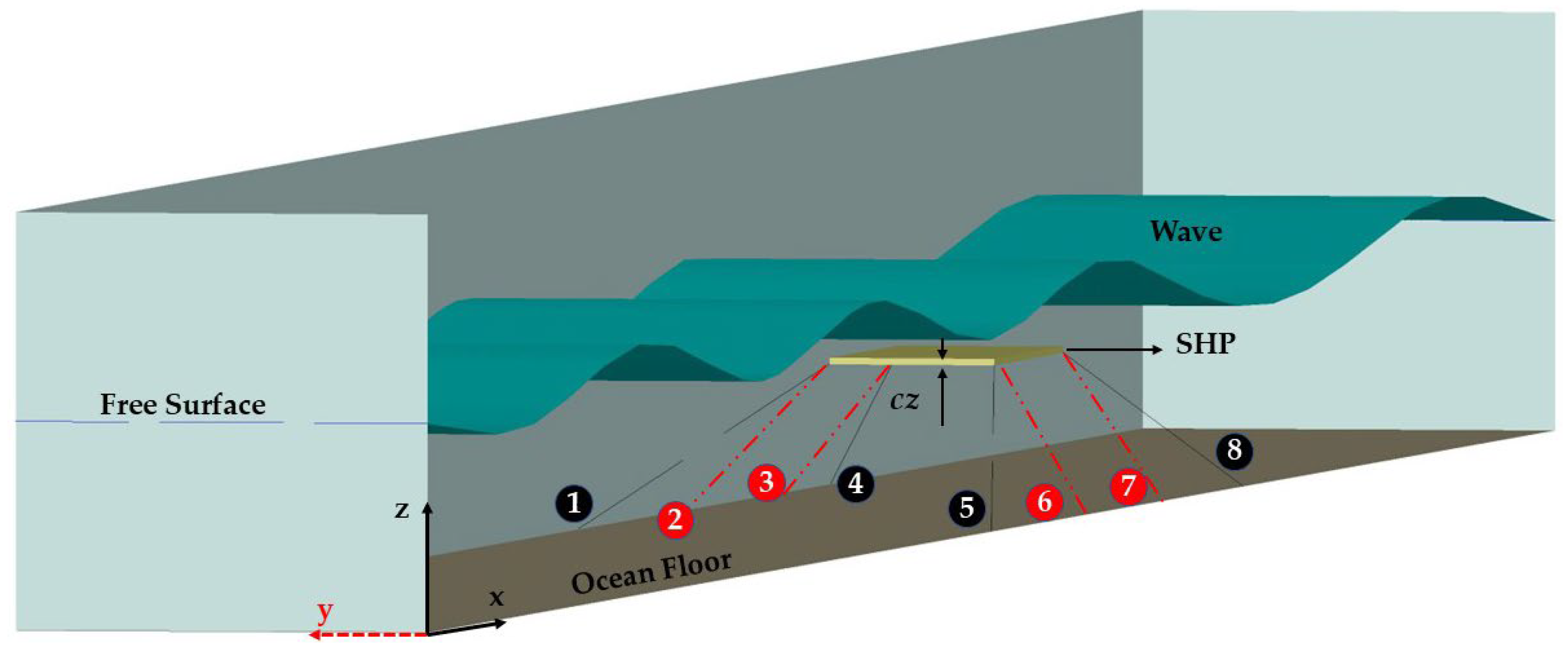
Figure 4.
Representation of the displacement Cz of the SHP due to the wave action and movement restrictions, in relation to the y- and x-axes, represented by cables 1, 2, 3, 4, 5, 6, 7, and 8.
In this sense, in the code, the inertia moments are defined as zero, so the mass distribution of the system does not make it susceptible to rotation around its principal axes when subjected to external forces. Displacement constraints are applied to the SHP, allowing translational movement only along the z-axis, while rotational movements around the x-, y-, and z-axes are restricted. This configuration simulates anchoring by cables 1 to 8, resulting in significant displacements only along the z-axis direction (Cz), as illustrated in Figure 4.
For the numerical simulations conducted to verify the numerical wave and efficiency analysis, 12,000 time-steps are used, with a time-step size of 0.0075 s, totaling 90 s of analysis. For model verification, 20,000 time-steps are used with the same time-step size of 0.0075 s, totaling 150 s of analysis, with both determined by convergence analysis. Each simulation took approximately 84 h to complete. The simulations are performed on a computer with the following specifications: Windows 10 operating system, Intel Core i5 processor, 32 GB of RAM, and 1 TB of storage, configured for data processing and system operations.
Seven simulations are conducted in two scenarios: one with an SHP in a non-oscillating condition and the other with an SHP device in an oscillating condition, both with the same NWT. In these simulations, the variations are limited due to the geometry of the SHP device and the incident wave characteristics, aiming to assess the efficiency of the WECs. A total of 14 simulations are conducted across the two scenarios, which totaled 1176 CPU hours.
The determination of SHP device displacement (Cz) caused by the incident flow is achieved using a UDF, associated with a dynamic mesh. The UDF is implemented in the ANSYS Fluent® software to define the properties of the SDOF, widely utilized in engineering and the analysis of dynamic systems [47], permitting displacement or rotation in only one direction or around an axis. This system is applied to the analysis of SHP movement through wave numerical impact.
2.4. Numerical Errors
The comparison between the numerical solution and the analytical solution based on Bernoulli’s equation is conducted by measuring the static pressure on the SHP, using the center of gravity as a reference. Numerical simulation plays a crucial role in analyzing scenarios that go beyond the inherent simplifications of the analytical solution. While Bernoulli’s equation provides an adequate description for ideal conditions, numerical modeling incorporates more complex phenomena, such as energy dissipation and fluid dynamic interactions, resulting in a more comprehensive and applicable analysis for real-world situations. However, due to the potential inaccuracies associated with numerical methods, analyzing the errors involved becomes essential. These errors are assessed by comparing the pressure differences between the analytical and numerical solutions, as well as in the process of the verification and validation of numerical models [13,17].
Ferziger and Peric [48] define numerical error (E) as the difference between the reference solution, which can be analytical or experimental, () and the numerical solution () obtained through a computational model. In this study, the numerical error represents the difference between the theoretical solution and the approximated solution obtained by a numerical method for .
By rewriting Equation (13) in terms of relative error (), a commonly used accuracy metric is obtained to assess the experimental or numerical results in relation to a given reference value:
The selection of the error metric plays a crucial role in determining the conclusions derived from a model analysis. The Root Mean Square Error (RMSE), the Root Mean Square (RMS), the Mean Absolute Error (MAE), and the Infinity Norm (N) are metrics utilized to evaluate model quality [49,50,51].
where n is the number of observed values, is the analytically obtained value, and is the predicted value for the numerical model.
The relative error () is used to compare the analytical and numerical pressure results () in the SHP, as it expresses the differences in percentage terms, facilitating the analysis of variables with different amplitudes. On the other hand, the evaluation of these errors () in the sample is carried out using the MAE, which provides a general measure of differences without excessively penalizing large deviations. The verification of the numerical wave is performed using the RMSE, which is more sensitive to high errors, allowing significant variations between profiles to be identified.
2.5. Domain Discretization
The discretization of the computational domain is a fundamental step in CFD, as it directly affects not only the numerical stability of the model but also the accuracy of the results in relation to the analytical solution. The creation of the computational domain is carried out in Workbench 2020 R2 software, which allows geometry construction using the Geometry module, and the generation of the discretized mesh through the Mesh module. After this step, the mesh is exported in a compatible format for the ANSYS Fluent® software, where the necessary configurations for the execution and analysis of the model are performed.
Mesh development is carried out using the Triangle Surface Mesher algorithm, widely recognized for its ability to generate high-quality triangular meshes [52]. This algorithm is particularly well suited for representing complex, irregular geometries, and free surfaces, making it ideal for models involving domains with non-uniform shapes, as are often encountered in fluid dynamics problems [53]. The algorithm employs an iterative refinement process, starting with a simple initial mesh and progressively refining the regions with a higher element concentration or more complex geometry. During the refinement process, the tool ensures the quality of the elements, preserving the geometric characteristics of the original mesh, and maintaining its integrity throughout.
To assess the sensitivity of the numerical solution to mesh discretization, a systematic mesh refinement study was carried out. Three mesh configurations were analyzed: a coarse mesh with approximately 30% fewer elements (565,633.6 elements), a reference mesh (808,048 elements), and a refined mesh with about 30% more elements (1,050,462 elements).
Simulations were conducted for each mesh configuration, keeping the boundary conditions, the mathematical formulation of the problem, and the convergence criteria unchanged. The variables of interest, velocity, pressure, and displacement, were evaluated for all mesh configurations, and the results were compared. The results showed that the difference between the reference mesh and the refined mesh was only 2.18%, while the variation between the reference mesh and the coarse mesh was 3.81%. These values indicate that the numerical solution is essentially mesh-independent. Therefore, the reference mesh was considered sufficiently refined for the purposes of this study.
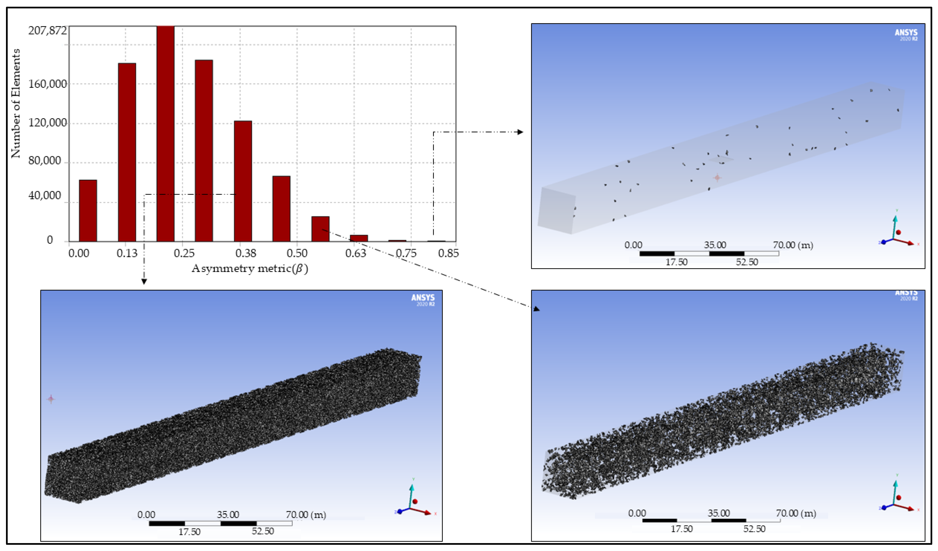
After the mesh generation, a quality analysis is performed directly within the Mesh tool using the asymmetry metric (β). This metric quantifies the distortion of the elements relative to their ideal shape [54], ensuring that the mesh maintains the geometric characteristics of the original geometry. Meshes with lower asymmetry values (β) guarantee better geometric conformity, which significantly contributes to the accuracy and stability of the numerical simulation results (Figure 5). In the case of the numerical wave tank (NWT), the mesh is generated considering the centralized position of the SHP within the channel, located at a depth of 9.0 m, which is 1.0 m below the free surface of the water, as shown in Figure 6.
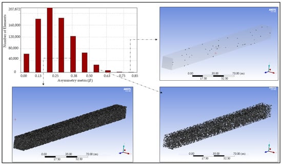
Figure 5.
Illustration of mesh quality and the distribution of its elements according to their values.
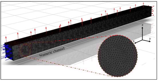
Figure 6.
Illustration of mesh details.
According to Moreira [54], the parameter is one of the main methods to verify numerical mesh quality, which determines how close each element is to its ideal shape. Based on the definition of , the value 0 indicates an equilateral element (best), the value 1 indicates a completely degenerate element (worst), and values between 0 and 1 are classified and presented in Table 2.
Table 2.
Classification of mesh element quality based on .
The statistical analysis by means of the parameter is employed utilizing the ANSYS software, allowing a detailed assessment of data distribution and the quality of the mesh generated during the simulation. As shown in Figure 5, the generated mesh presents the maximum and minimum values of equal to 0.836100 and 0.000149, respectively.
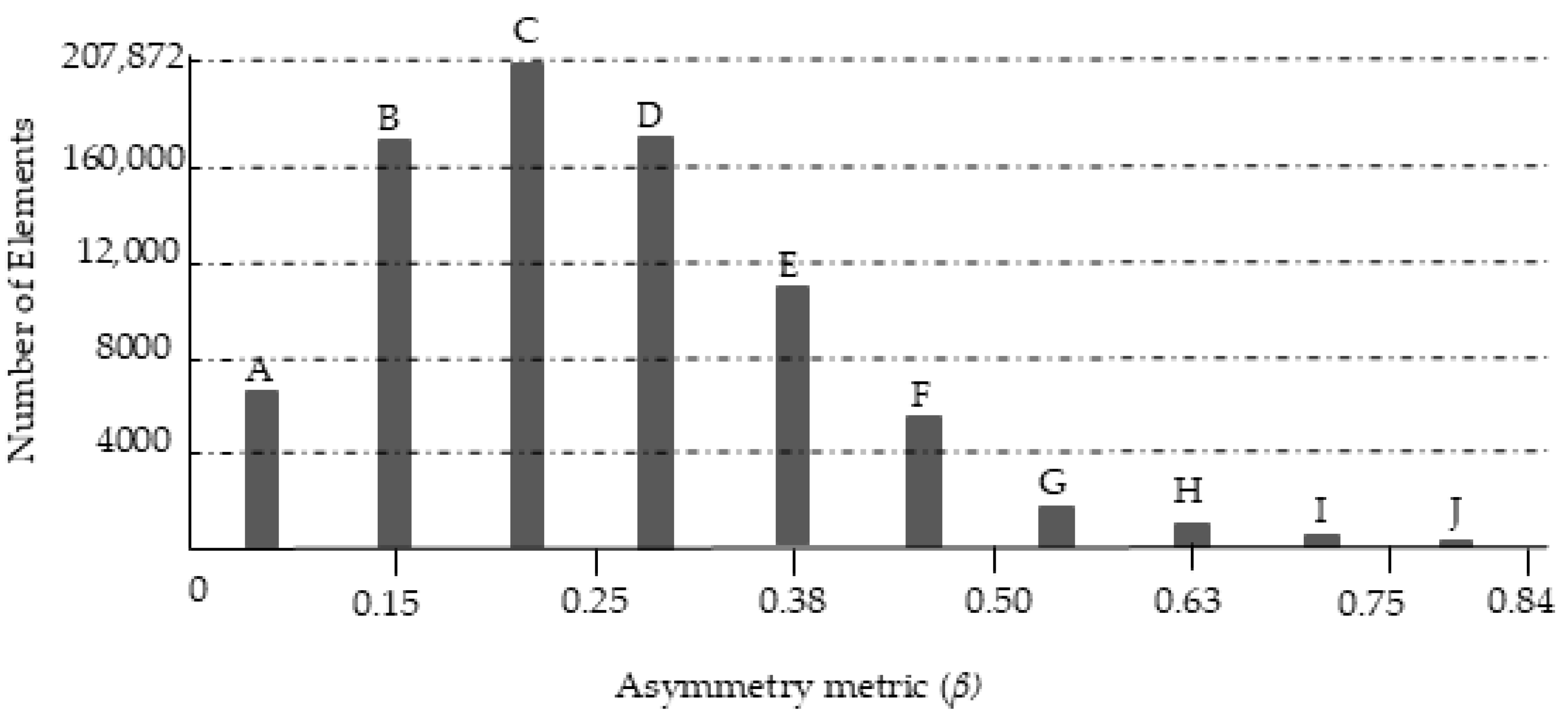
The proposed model, composed of 808.048 elements, is found to remain within acceptable quality ranges, with distributed elements in 10 categories (Figure 7).

Figure 7.
Distribution of mesh elements in categories A, B, C, D, E, F, G, H, I, and J, according to values.
Table 3 illustrates the mesh elements according to intervals, categorized by the quality of the elements and the quantity corresponding to each category. This provides a clear view of mesh quality, facilitating the analysis of the integrated elements of the models, highlighting the predominant elements in the categories of Good and Excellent.
Table 3.
The distribution of mesh elements according to the intervals, classifying the quality of the elements and the corresponding quantity in each category.
2.6. Parameters of Interest
The divisions of the NWT are established based on the study by Seibt et al. [13] and are illustrated in Figure 8. The channel is segmented into three regions: Region 1 consists of the wave propagation zone and has a length of 2λ, equivalent to 120.8 m and 140.8 m; Region 2, with a length L, varies depending on the SHP geometry; and Region 3 has a length of 4λ, corresponding to 241.6 m and 281.6 m, respectively. This region contains the numerical beach, starting at the initial position and extending to the end of the channel (hydrostatic profile), with a length of 120.8 m and 140.8 m, which corresponds to 2λ.
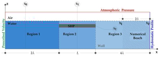
Figure 8.
Representation of the NWT divided into three regions, highlighting the SHP device and the probes , , and , positioned at the points of interest for parameter monitoring and the presence of the numerical beach in Region 3.
To monitor the necessary parameters for determining the theoretical efficiency of the device φ, three probes are created and designated as , and (Figure 8). The free surface elevation is determined using a planar probe , located 5 m from the wave generator (prescribed velocity). To measure the average velocity () and the maximum velocity () of the flow beneath the device, a linear monitor is used, positioned between the water surface and the bottom of the numerical channel, passing through the center of the SHP. The displacement ( and static pressure () are measured using the device itself as a monitor, submerged 1 m, represented by .
The determination of the parameter φ for the SHP is based on the theoretical framework presented by Graw [55] and Orer and Ozdamar [18], combined with the data obtained during the simulation. The steps described in these studies are strictly followed in the calculation, incorporating the monitored pressure and flow information.
Theoretical efficiency (φ) is a measure of the performance of an ideal process or system that does not consider energy losses or other practical limitations that may occur in real life. It is calculated by considering the maximum possible output or production that would be achieved under ideal conditions, without any energy or material losses [28]. It can be obtained as the ratio between the average power available in the flow and the average power associated with the wave , following the methodologies established in [18,55]:
where is calculated considering the wave power (W) incident on the WEC, using the second-order Stokes theory [56]. The average available power on the device can be calculated as described in [57,58]:
In this Equation (26), p represents the static pressure (Pa) on the SHP, the term (ρu2/2) represents the dynamic pressure (Pa), d is the height of the SHP (m), h is the water depth (m), and is the width of the SHP (m). Static pressure monitoring on the SHP was conducted directly, tracking the oscillatory motion of the structure, using its center of gravity as a reference. The u velocity was measured using the linear monitor .
3. Results and Discussion
3.1. Verification of the Numerical Model
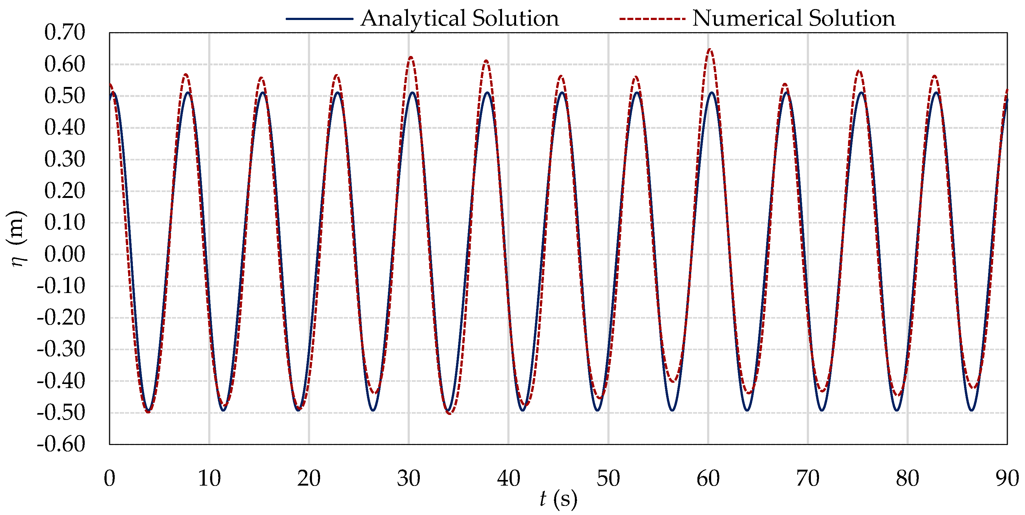
Regular waves were initially generated in the NWT and simulated without the presence of the SHP to verify the numerical wave. The wave spectrum referenced in this article corresponds to the representation of the significant wave height derived from regular waves with a period T = 7.5 s, characteristic of the area of interest [59]. This approach was adopted to simplify the numerical verification process, focusing on the energy contribution of the most relevant waves without the need to simulate the full complexity of a complete spectrum. Specifically, regular waves were generated in the NWT with the following characteristics: H = 1.0 m, , h = 10.0 m, and T = 7.5 s. These conditions were selected for being representative of the predominant waves in the area of interest, enabling an initial analysis based on idealized conditions. Figure 9 illustrates the qualitative comparison for the obtained results monitored by the probe line (see Figure 8) of the free surface elevation, with the analytical solution defined by Equation (9) and used as a reference.
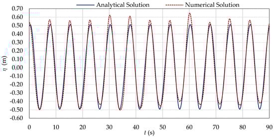
Figure 9.
Comparison of the analytical and numerical solution for the free surface elevation, considering a significant wave height of H = 1.0 m and period of T = 7.5 s.
Considering the 90 s simulation interval, based on the second-order Stokes theory and the laminar flow model, differences between the analytical and numerical curves were observed. These differences could be attributed to interference from the side walls of the 3D NWT, which, by interacting with the waves, caused additional disturbances in their propagation. These disturbances resulted in variations in the numerical results compared to the analytical solution, which assumed ideal conditions without considering such interference. To evaluate the accuracy of the obtained results, the errors in the model were quantitatively calculated, as shown in Table 4.
Table 4.
Comparison of the errors between the numerical and analytical solutions for different time-step sizes.
The data in Table 4 were analyzed based on error values calculated for specific time intervals. The MAE showed a reduction over time: 0.0507 m (20 to 40 s), 0.0472 m (40 to 60 s), 0.0439 m (60 to 80 s), and 0.0405 m (80 to 90 s). This trend indicates that the numerical solution gradually approaches the analytical one. The RMSE followed a similar pattern, decreasing from 0.0626 m (20 to 40 s) to 0.0456 m (80 to 90 s), with intermediate values of 0.0595 m (40 to 60 s) and 0.0532 m (60 to 80 s). This progressive reduction confirmed good convergence between the numerical and analytical solutions. The differences in the infinity norms, which measured the largest absolute error in each interval, varied more significantly: 0.1122 m (20 to 40 s), 0.1290 m (40 to 60 s), 0.1371 m (60 to 80 s), and 0.0526 m (80 to 90 s). Despite peaks in the intermediate intervals, the significant drop in the final interval demonstrated substantial improvement in maximum errors. Finally, the RMS of the numerical error was identical to the analytical RMSE across all intervals, reinforcing consistency and compatibility between the numerical and analytical solutions.
These results reinforced that, although there was good agreement between the numerical and analytical solutions, some deviations could be observed. According to Equation (21), the RMSE was 5.75%. Despite this, it was noted that, for most of the simulation, the numerical and analytical curves agreed significantly, although the upper points of the numerical curve exceeded the peaks determined by Equation (9), while the lower points fell below.
The acceptable error for this study was defined considering the good agreement between the numerical and analytical solutions and the progressive reduction of errors over time. The RMSE, with a maximum value of 5.75%, was used as the main reference to determine the model’s accuracy. Additionally, the MAE and infinity norm showed a decreasing trend as the simulation time increased, demonstrating a consistent convergence of the solutions. These values align with the objectives of this study, which aimed to reproduce the essential characteristics of the phenomenon. Thus, the acceptable error was established at up to 6%, encompassing the highest observed RMSE and ensuring that the numerical results adequately represented the expected behavior.
The difference in the upper and lower peak values of the numerical curve compared to the theoretical one could be explained as the result of a complex interaction between fluid dynamics and the limits imposed by the lateral boundary conditions. Although V (x, z, t) = 0 was imposed on the lateral walls, this did not entirely eliminate the indirect effects of these conditions, which could be attributed to various interconnected factors.
The lateral walls may partially reflect the wave energy, generating constructive and destructive interference that distorts the amplitudes, resulting in higher upper peaks and smaller lower peaks. Additionally, the dimensions of the three-dimensional domain may induce natural resonance effects, locally amplifying or attenuating the wave amplitudes and contributing to the observed discrepancy. The presence of the walls also influenced the pressure field near the boundaries, redistributing wave energy and altering their propagation and simulated amplitudes. Finally, spatial and temporal discretization could introduce cumulative errors, and even refined meshes may have limitations that affect the accuracy of the simulated values.
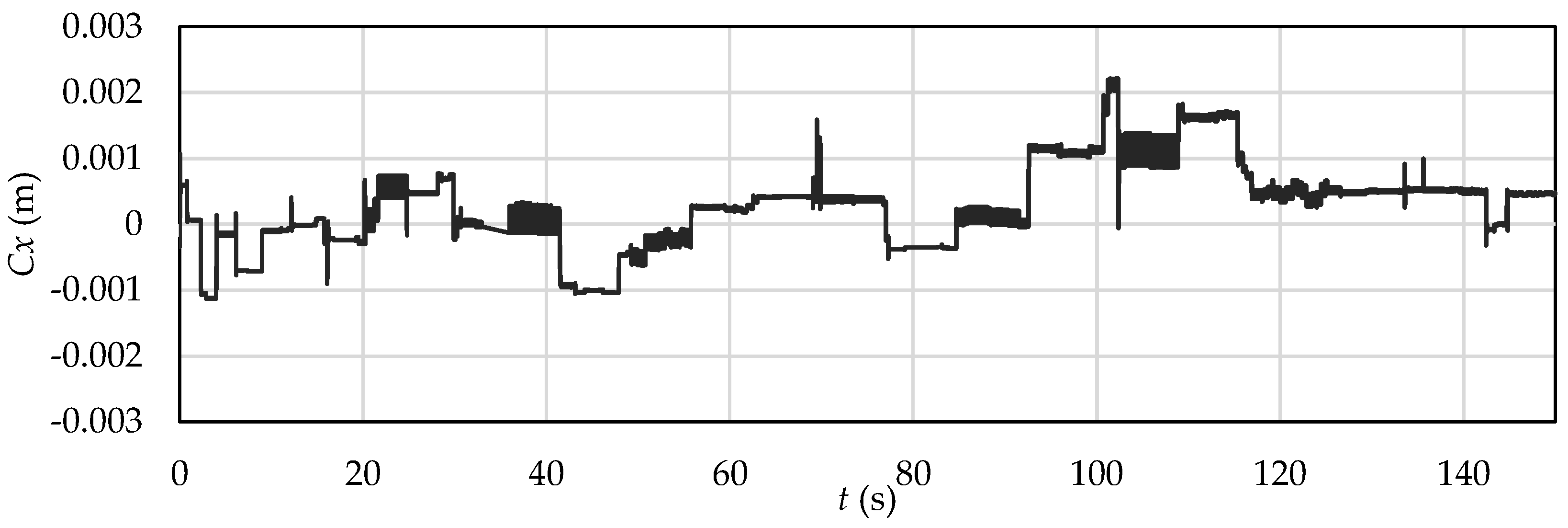
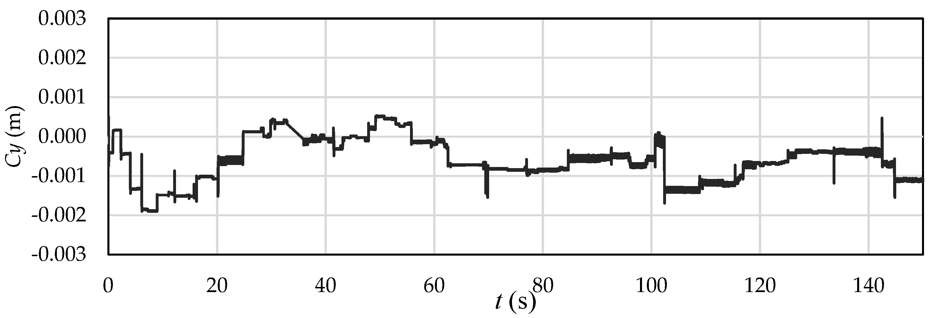
The verification of the SHP was conducted using the same characteristics employed in the verification of the numerical wave, with the difference being the presence of an SHP with the dimensions L = 10.0 m, B = 8.0 m, and e = 0.32 m, centered in the NWT. Regarding the displacements of the SHP in relation to the x- and y-axes where movement restrictions were applied, no significant movements were observed in the x-component (Cx) and the y-component (Cy), as shown in Figure 10 and Figure 11, respectively.
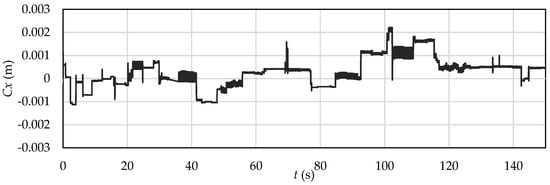
Figure 10.
SHP device oscillation (Cx) in the x-axis direction (m).
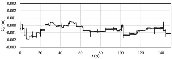
Figure 11.
SHP device oscillation (Cy) in the y-axis direction (m).
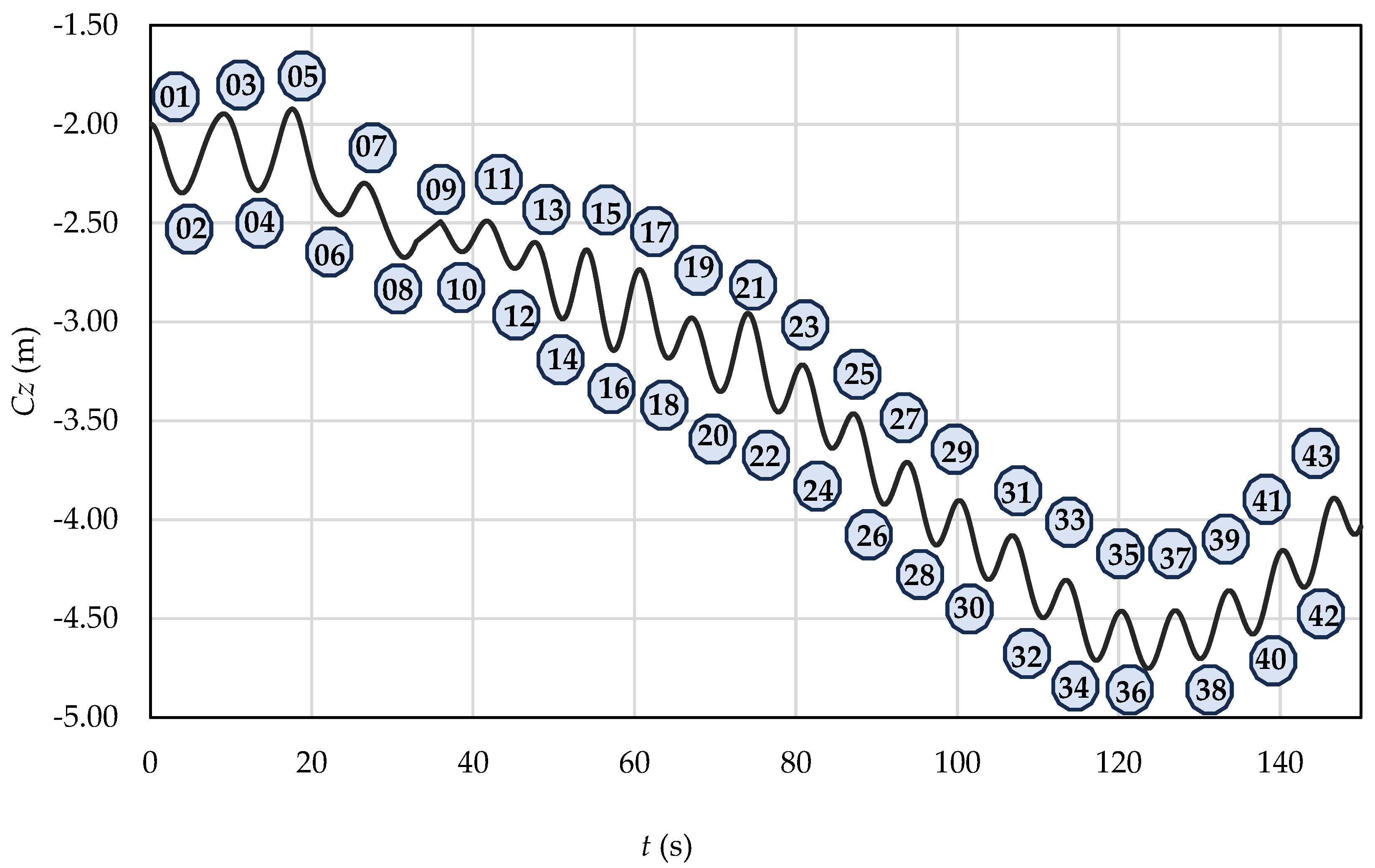
For the simulation considering the incidence of 20 waves (20,000 time-steps of 0.0075), oscillatory movements of the SHP in the direction of the z-axis component (Cz) were observed. The device began its oscillating motion from the level of −2.16 m. In the first 20 s, it oscillated between the level of −2.5 m and its initial motion level. Subsequently, it entered a descending oscillatory motion, reaching levels of −3.0 m and −4.0 m at t = 56 s and t = 96 s, respectively. The descending oscillatory motion reached its maximum submersion level of −4.75 m at t = 120 s, with a total displacement of 2.59 m, and then initiated an oscillating return motion toward the starting point, as shown in Figure 12.
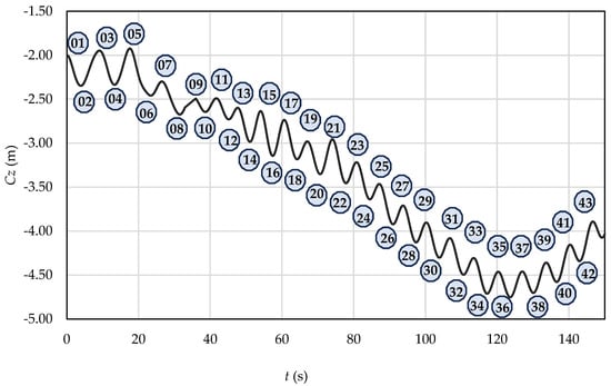
Figure 12.
SHP device oscillation (Cz) in the z-axis direction (m).
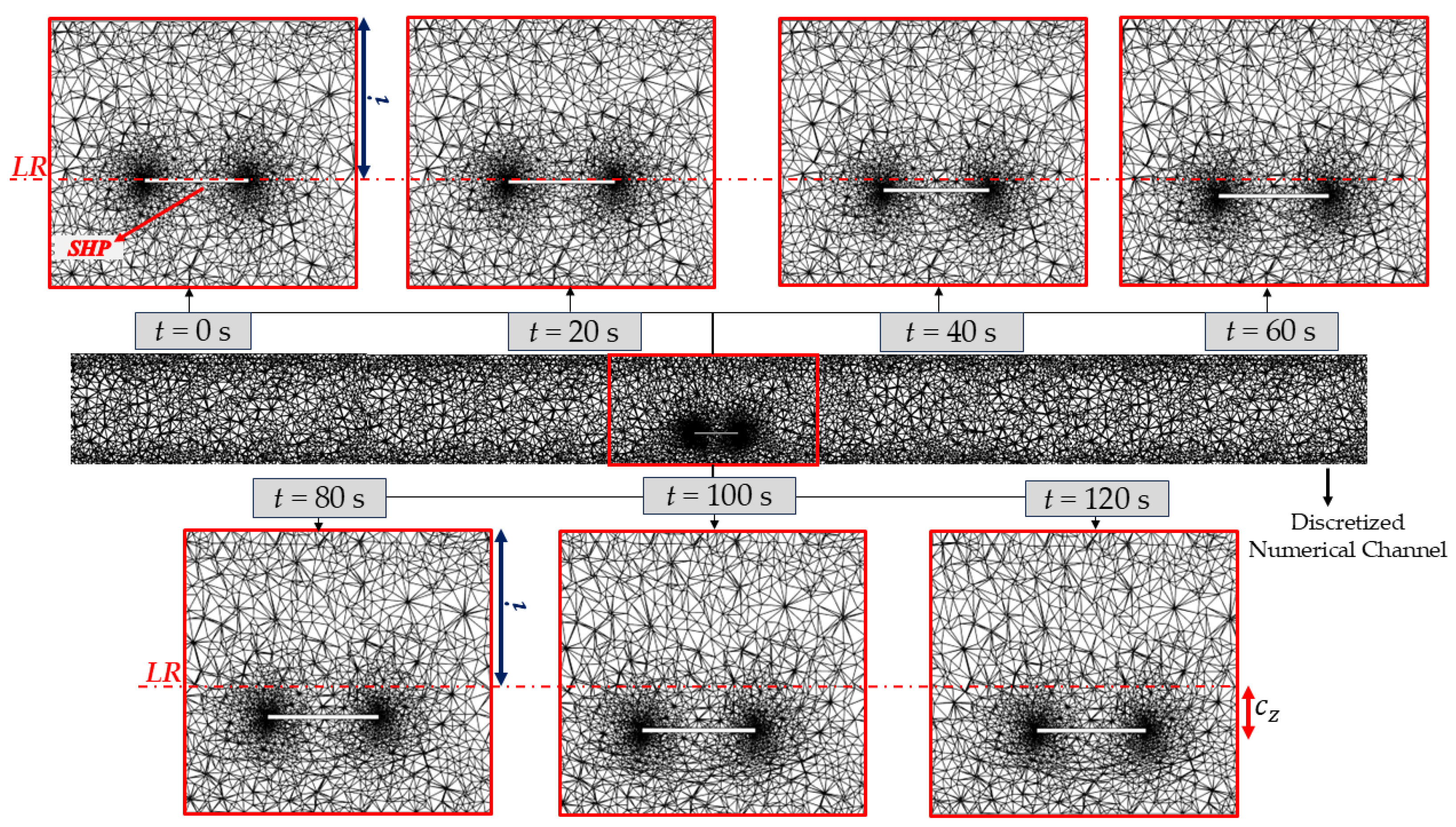
Complementing the analysis of the SHP’s oscillatory motion, Figure 13 shows the deformation of the numerical mesh at different instants of the simulation: t = 0 s, t = 20 s, t = 40 s, t = 60 s, t = 80 s, t = 100 s, and t = 120 s. The displacement Cz could be observed from a reference line (RL), positioned at a distance i from the upper surface of the numerical channel, passing through the SHP in its initial position.

Figure 13.
Illustration of the mesh deformation and the oscillation Cz of the SHP at the time instances t = 0 s, t = 20 s, t = 40 s, t = 60 s, t = 80 s, t = 100 s, and t = 120 s, with the reference line (RL) positioned over the SHP at rest (t = 0 s), located at a distance i from the upper boundary of the channel.
In the first instants, the deformation was more pronounced in the region near the surface, following the initial oscillatory movement of the SHP. As time increased, the mesh deformation became more evident as the device approached its maximum submersion level of −4.75 m.
The verification process of the dynamic model consisted of comparing the values of , determined analytically using Equation (18), developed by Bernoulli, with values obtained numerically. For this, 43 inflection points were considered, where a change in direction occurred in the upward or downward movement of the SHP during the oscillatory motion of the device, as shown in Figure 12.
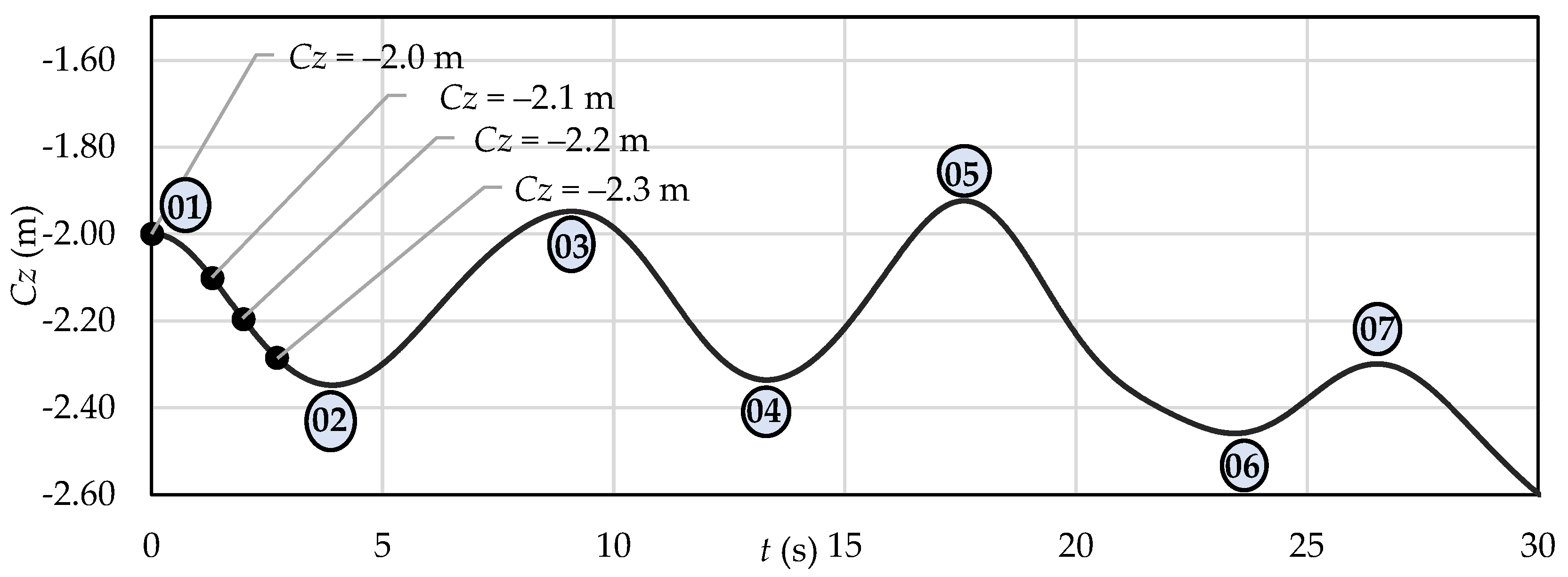
With the inflection points defined, Cz values were selected at every 0.1 m between the inflection points (Figure 14). This generated a total of 134 displacement values of the SHP, which enabled the calculation of the analytical values of . The results obtained through Equation (20) revealed a significant variation in between the analytical and numerical results of over time.
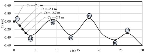
Figure 14.
Representation of Cz values (m) for the points selected between inflection points 01 and 02.
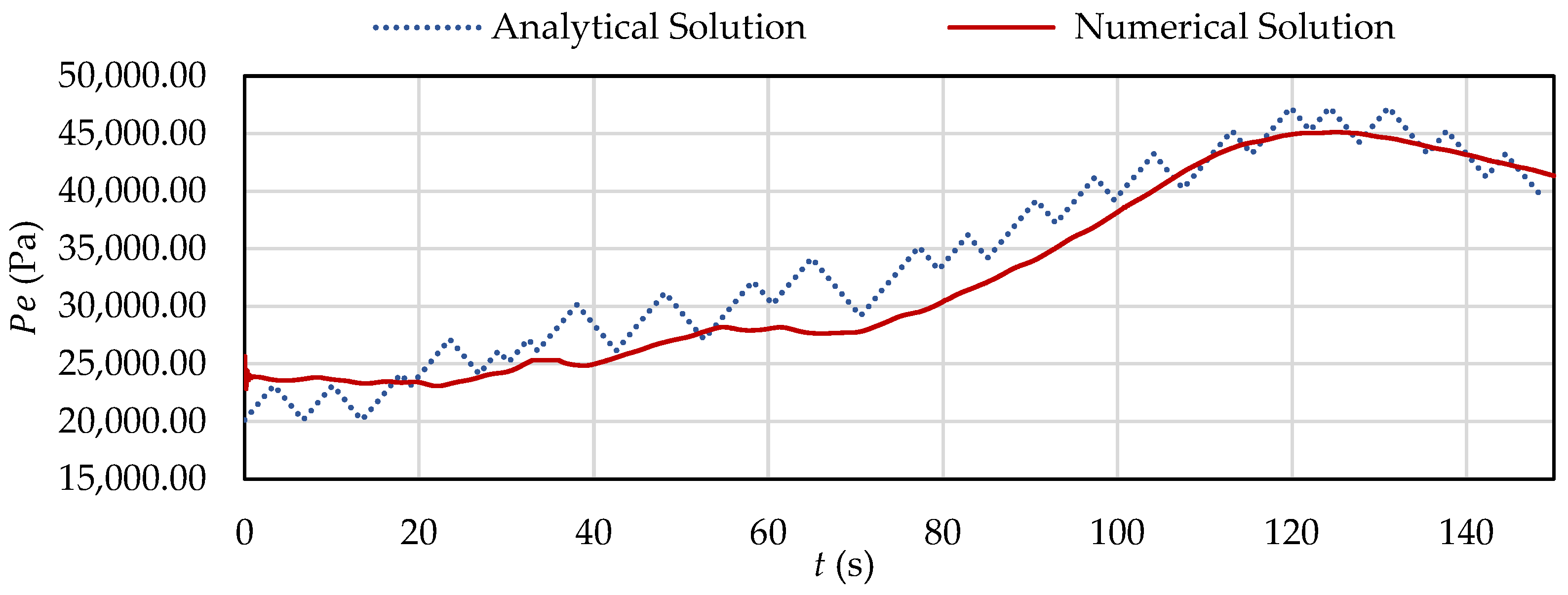
The observed percentage oscillation varied between positive and negative values. Based on these results, the MAE was used for data analysis, as described in Equation (23). The obtained MAE was approximately 6.89%, indicating that, on average, the numerical values of showed a difference of about 6.89% compared to the analytical values. Moreover, the generated curves demonstrated a similar behavioral trend, as illustrated in Figure 15.
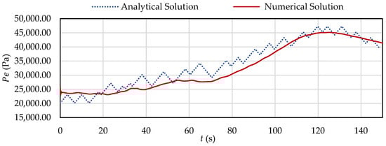
Figure 15.
Variation of during the oscillatory motion of the SHP.
Therefore, based on the verification results presented one can infer that both the computational model for the generation of regular waves and the one for the movement of the SHP under the incidence of these waves were duly verified and can be used for the proposed case study.
3.2. Evaluation of the Efficiency of the SHP Device in Non-Oscillating and Oscillating Modes
This section analyzes the impact of the geometric configurations of the SHP device on efficiency and hydrodynamic performance, considering the different characteristics of the waves used. The analysis aims to understand how these variables influence the determination of φ, as design changes can directly affect hydrodynamic performance and system optimization. To achieve this, various theoretical scenarios will be explored, allowing for the evaluation of the SHP’s response under different conditions.
The chosen configurations reflected real-world situations, such as offshore platforms and submerged structures, where efficiency was intrinsically linked to geometric adequacy. For instance, reducing the thickness (e) could enable the use of lighter and more economical materials, while width adjustments in width (B) were useful for meeting specific spatial constraints.
For this purpose, seven cases were analyzed, varying the characteristics of the numerical wave, such as H and , as well as the dimensions of the SHP, including L, B, and e, as detailed in Table 5. The simulations encompassed both NO and O conditions of the SHP, totaling fourteen scenarios evaluated.
Table 5.
Details of the simulated cases.
By varying the geometric parameters of the SHP and the wave characteristics, it was possible to determine the values of and for both NO and O conditions (Table 6), enabling a comparative analysis of hydrodynamic performance across different scenarios.
Table 6.
Values of and for the NO and O conditions.
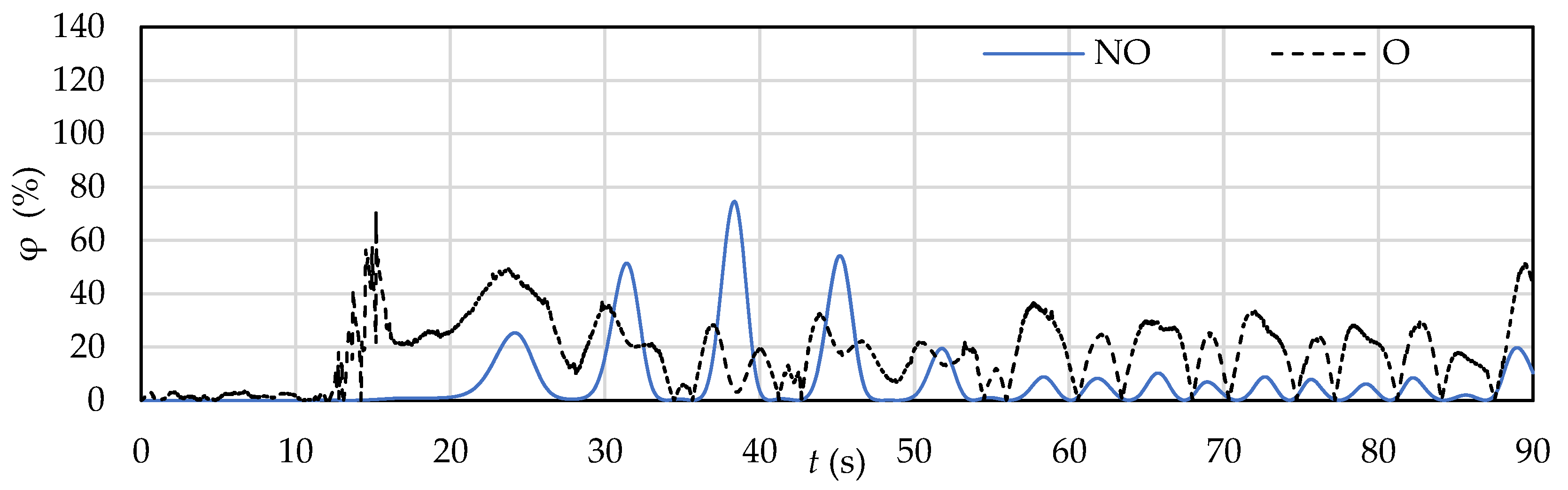
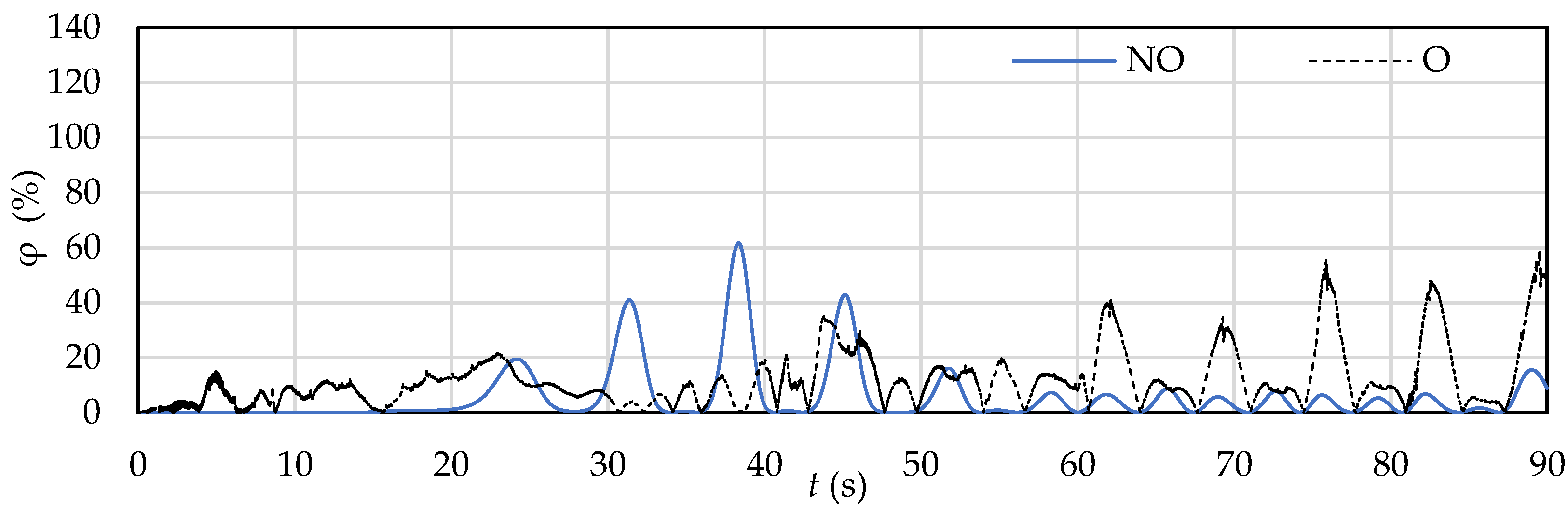
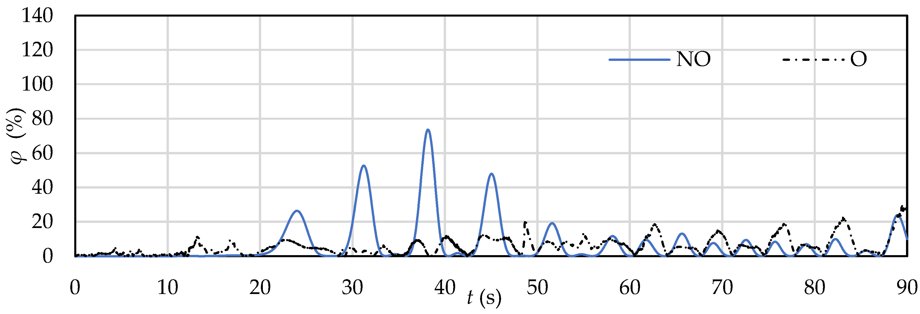
In the seven cases discussed, the time-step size considered was 0.0075 s. In the first three cases analyzed, the characteristics of the numerical wave remained constant, while the geometric parameters of the SHP—L, B, and e—were altered. In Case 1, the obtained values of φ served as a reference, as they represent the initial configuration of the verified model, without alterations to the geometric parameters. The analysis of Figure 16, Figure 17 and Figure 18 showed that these geometric changes contributed to the decrease in φ over time in the O condition. On the other hand, it was found that the NO condition consistently presented lower values of φ, indicating a lower intensity of the hydrodynamic interaction compared to the O condition.
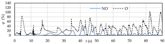
Figure 16.
Case 1: variation of the φ for the NO and O conditions of the device.
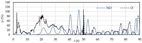
Figure 17.
Case 2: variation of the φ for the NO and O conditions of the device.
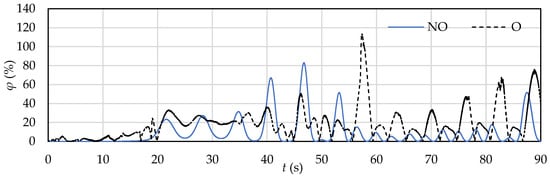
Figure 18.
Case 3: variation of the φ for the NO and O conditions of the device.
In Case 2, the thickness was reduced to e = 0.16 m, resulting in a decrease in φ. This was attributed to the lower weight and, consequently, greater buoyancy, but it was not enough to improve energy conversion, leading to an average efficiency () of 22.68%. In Case 3, the width was reduced to L = 8 m, with e = 0.32 m remaining constant, which also caused a drop in efficiency, with a value of 18.73%. In both cases, the observed efficiencies were lower than the reference value of 27.48% from Case 1. These results suggest that the reduction in the geometric parameters of the SHP, which alters buoyancy, hinders energy conversion, possibly by limiting the energy transfer between the wave and the device.
In Case 4, the highest value of φ was observed for the O condition, as illustrated in Figure 19. This result was achieved due to the simultaneous reduction of the numerical wave height H, the length L, and the e of the SHP. The decrease in H reduced the wave energy, while the smaller geometric dimensions of the SHP contributed to the increase in φ, possibly due to greater displacement in the z-direction, which favored a more balanced distribution of forces and a more efficient interaction with the wave. In this scenario, the was 35.68%, demonstrating that the geometric configuration and wave characteristics positively influenced performance compared to Cases 1, 2, and 3.
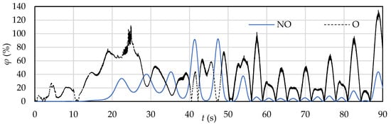
Figure 19.
Case 4: variation of the φ for the NO and O conditions of the device.
In contrast, for the NO condition, the values of φ were substantially lower in Cases 1, 2, and 3 compared to Case 4 in the O condition, with an average efficiency of 12.57%, and with a value of =29,986.57 W, which was lower than the values obtained in the other cases (Table 6). This reduction could be attributed to the lower hydrodynamic interaction between the wave and the SHP, resulting from the geometric configuration, which limited the energy transfer between the wave and the dynamic response of the structure.
In Cases 5 and 6, variations in the thickness (e) of the SHP with a length of 12 m were made when subjected to a wave with H = 1.0 m and λ = 70.40 m. The results indicated that the reduction in e resulted in a loss of efficiency of the device, as observed in Figure 20 and Figure 21. The reduced thickness of the SHP in Case 6 resulted in lower weight and greater buoyancy; however, this did not enhance the efficient conversion of wave energy. As a result, there was increased energy dissipation and a less effective structural response.

Figure 20.
Case 5: variation of the φ for the NO and O conditions of the device.
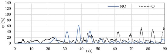
Figure 21.
Case 6: variation of the φ for the NO and O conditions of the device.
Both Case 5 and Case 6 achieved average efficiencies lower than Case 1, with = 18.09% and = 11.75%, respectively. Furthermore, the NO condition of the SHP proved to be even less efficient, with = 6.94% for Case 5 and = 5.57% for Case 6.
In Case 7, simulations were conducted by varying the three dimensions of the SHP: L = 8 m, B = 12 m, and e = 0.32 m, when the device was exposed to a numerical wave with H = 1.5 m and λ = 70.40 m. Under these conditions, the SHP exhibited lower efficiency, with a value of = 5.74% in the oscillating condition (O), as shown in Figure 22. This result could be explained by the combination of an increased width (B) and the higher wave height (H).
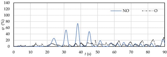
Figure 22.
Case 7: variation of the φ for the NO and O conditions of the device.
The higher wave height resulted in more energy being transferred to the SHP, but the change in geometry, with an increase in width and maintenance of thickness, may have impaired the dynamic response of the device. The structure, treated as a rigid body, may have had its ability to move in the z-axis direction limited due to the increase in width. This occurred because the larger width may have altered the distribution of forces, restricting the structure’s response to the waves, which resulted in a less efficient conversion of wave energy.
On the other hand, the NO condition exhibited a higher value of = 6.83%, compared to the O condition. This could be attributed to the configuration which resulted in a higher value of = 147,343.50 W in the NO condition relative to = 123,825.84 W observed in the O condition. This result suggests that the NO condition generated a more efficient interaction between the wave and the structure, leading to a higher energy transfer. This behavior was observed only in this case, among the seven simulated cases (Table 6).
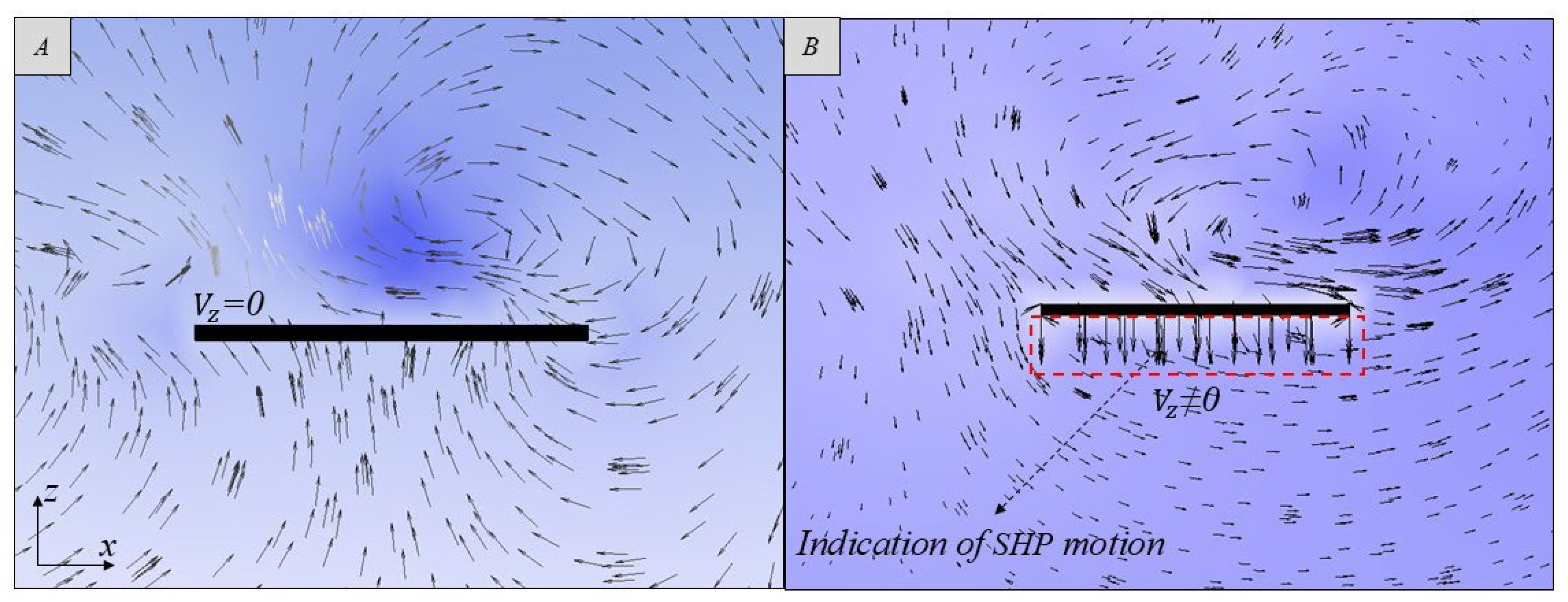
It is noteworthy that, although this study primarily analyzed the average and maximum velocities beneath the SHP, a detailed understanding of the velocity field around the device is equally essential. The velocity field provided comprehensive information about the flow pattern around the device, allowing for the identification of turbulence zones, recirculation, and other hydrodynamic phenomena that could affect the system’s performance (Figure 23). This understanding is crucial not only for optimizing the efficiency of wave energy transfer but also for ensuring the structural stability of the device [60,61].
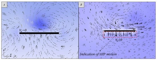
Figure 23.
Velocity vectors in the vertical direction () of the SHP, Case 1, under NO condition (A) and O condition (B) at t = 90s.
These hydrodynamic phenomena were clearly observed in this study, emphasizing the importance of a detailed analysis of the velocity field around the SHP. Furthermore, Figure 23 allows for the visualization of the displacement vectors of the SHP, highlighting its vertical movement as it is struck by the wave. This graphical representation not only illustrated the behavior of the SHP in response to the wave–device interaction but also offered insights into the flow patterns around it, aiding in the identification of critical areas of hydrodynamic impact.
The average velocity ( of the flow under the SHP and values for the simulated cases, organized in Table 7, showed that the oscillating (O) condition could have a significant impact on both ( and () of the SHP. However, the relationship between these factors was not straightforward and may vary according to the specific characteristics of each case, including the geometry used and the numerical wave properties.
Table 7.
Average velocity and average efficiency () values determined for the NO and O conditions.
Table 8 presents the values determined with the SHP under NO and O conditions, revealing significant variations across the analyzed cases. In Case 1, = 23.66 m/s was substantially higher, where = 4.72 m/s, indicating a significant increase in velocity intensity due to the influence of SHP geometry. In other cases, such as Case 3, the values were very similar, with = 21.26 m/s and = 21.43 m/s, suggesting that the impact of the SHP was less significant in this scenario. Case 4 exhibited significant behavior, resulting in = 88.09 m/s, compared to = 14.66 m/s, highlighting a notable increase in velocity due to the SHP’s geometric characteristics. These results emphasized that the shape and configuration of the SHP play a considerable role in velocity dynamics, especially under specific initial or operational conditions.
Table 8.
Maximum velocity values under SHP () values determined under NO and O conditions.
These results highlight that the geometry and configuration of the SHP have a significant influence on velocity dynamics, especially due to initial conditions, such as the initial state of the water, and operational conditions, such as wave intensity and the vertical displacements of an SHP during operation.
4. Conclusions
In this study, a numerical and geometric analysis was conducted on an SHP device proposed to be installed on the coast of the state of Rio Grande do Sul, Brazil, submerged at 1 m depth in a location with a total depth of 10 m. The main goal of this analysis was to verify the model considering the wave characteristics of this location and to assess how different geometries impact the performance of an SHP device under O and NO conditions. In summary, this study aimed to identify the most efficient geometry to optimize electricity generation in each specific scenario.
The fluid flow was considered transient with a laminar regime. Additionally, the fluid was treated as biphasic (air and water), with this interaction handled using the VOF method. In the numerical solutions, the conservation equations for mass, momentum, and volume fraction were solved using the FVM.
This study concluded that the model used for verifying the numerical wave, without the presence of the device, agreed with the analytical solution, considering the stabilized wave generation time. It was observed that the RMS of the numerical error showed higher values in the initial intervals (20 to 40 s) with a value of 0.0626, and tended to decrease over time, reaching 0.0456 in the final interval (80 to 90 s). This reduction indicated that as time progressed, the numerical error in the simulation decreased. Ultimately, the RMS of the numerical error was identical to the analytical RMSE across all intervals, reinforcing the consistency and compatibility between the numerical and analytical solutions.
This reduction in error could be attributed to the stabilization process of the numerical model, which was configured with the use of a numerical beach for wave energy dissipation. During the initial moments of the simulation, the system might have been adjusting to its initial conditions, resulting in larger discrepancies. As the simulation progressed, the model configuration stabilized, leading to a greater agreement between the numerical results and the analytical solution. Although the phenomenon of reflection at the numerical beach was an important factor, the observed reduction in error was more related to the stabilization of the simulated process than to the complete absorption of waves by the numerical beach.
The numerical model was validated with the SHP centered in the NWT. Seven distinct cases were analyzed, varying parameters such as the geometry of the SHP and the characteristics of the numerical wave under NO and O conditions. It was observed that these parameters influenced the SHP’s efficiency values and the velocity beneath the analyzed structure. The analysis of the SHP device’s efficiency under NO and O conditions revealed notable differences. Generally, the system’s average efficiency, represented by , tends to be higher under O conditions, except for in Case 7.
In Case 1, for example, the efficiency in the O condition = 27.48% was significantly higher than in the NO condition = 5.54%, highlighting the significant effect of oscillation on the device’s performance. Case 4 showed an even more pronounced difference, with efficiency increasing from 12.57% to = 35.68% when comparing the NO and O conditions, respectively. However, Case 7 presented an inversion of this pattern, with efficiency in the NO condition = 6.83% being higher than in the O condition = 5.74%. This behavior suggests that, although O conditions generally favor the SHP device’s efficiency, geometric factors or other specific variables may negatively influence performance in certain scenarios.
Case 4 achieved the highest efficiency value, with = 35.68% and = 88 m/s, indicating that the geometric configuration and wave conditions in this case were the most suitable for optimizing system performance. Finally, the results of the simulated cases highlight the importance of a geometric analysis of an SHP device and knowledge of the installation region. These factors directly influenced efficiency and, consequently, the feasibility of implementing the device.
Although this study presents relevant results under controlled conditions, certain aspects of the model could be further improved in future work. For instance, the use of regular waves provides only an approximate representation of the complexity of the marine environment, and it is recommended that future studies examine the device’s behavior under irregular wave conditions. Furthermore, the flow was treated as laminar, which is appropriate for the conditions analyzed; however, incorporating turbulence models in future simulations could lead to a more comprehensive understanding of the phenomena involved. These potential extensions may contribute to a deeper insight into the system’s performance across a range of operating scenarios.
Author Contributions
Conceptualization, R.C.B., M.d.N.G. and L.A.I.; methodology, R.C.B., M.d.N.G. and L.A.I.; software, R.C.B., M.d.N.G. and L.A.I.; validation, R.C.B., M.d.N.G. and L.A.I.; formal analysis, L.A.I., E.D.d.S. and L.A.O.R.; investigation, R.C.B., M.d.N.G. and L.A.I.; resources, L.A.O.R., E.D.d.S., M.d.N.G. and L.A.I.; data curation, R.C.B., M.d.N.G. and L.A.I.; writing—original draft preparation, R.C.B., M.d.N.G. and M.R.d.O.; writing—review and editing, R.C.B., M.d.N.G., L.A.I., M.R.d.O., E.D.d.S. and L.A.O.R.; visualization, L.A.O.R., E.D.d.S., M.d.N.G. and L.A.I.; supervision, M.d.N.G. and L.A.I.; project administration, M.d.N.G. and L.A.I.; funding acquisition, L.A.O.R., E.D.d.S., M.d.N.G. and L.A.I. All authors have read and agreed to the published version of the manuscript.
Funding
This research was funded by the Research Support Foundation of the State of Rio Grande do Sul—FAPERGS (Public Call FAPERGS 07/2021—Programa Pesquisador Gaúcho—PqG—21/2551-0002231-0) and the Brazilian National Council for Scientific and Technological Development—CNPq (Processes: 125941/2024-2, 309648/2021-1, 307791/2019-0, 308396/2021-9, 440010/2019-5, and 440020/2019-0).
Data Availability Statement
Data can be accessed upon request to the authors.
Acknowledgments
R.C. Batista thanks the Federal Institute of Paraná (IFPR) for access to the computer labs and the Federal Institute of São Paulo (IFSP) for encouraging capacity building. The authors thank FAPERGS and CNPq for the financial support.
Conflicts of Interest
The authors declare no conflicts of interest.
Appendix A
| Code UDF #include “udf.h” DEFINE_SDOF_PROPERTIES (stage, prop, dt, time, dtime) { // Define the mass of the rigid body prop[SDOF_MASS] = Mass; // Defining the SHP mass // Define moments of inertia as zero prop[SDOF_IXX] = 0; // Moment of Inertia about the X-axis (zero) prop[SDOF_IYY] = 0; // Moment of Inertia about the Y-axis (zero) prop[SDOF_IZZ] = 0; // Moment of Inertia about the Z-axis (zero) // Define the acting loads as needed prop[SDOF_LOAD_F_Z] = load; // Z-axis force // Displacement constraints prop[SDOF_ZERO_TRANS_X] = TRUE; // Movement restricted along the X-axis prop[SDOF_ZERO_TRANS_Y] = TRUE; // Movement restricted along the Y-axis prop[SDOF_ZERO_TRANS_Z] = FALSE; // Allows movement in the Z direction // Rotation restrictions prop[SDOF_ZERO_ROT_X] = TRUE; // Rotation restricted around X-axis prop[SDOF_ZERO_ROT_Y] = TRUE; // Rotation restricted around Y-axis prop[SDOF_ZERO_ROT_Z] = TRUE; // Rotation restricted around Z-axis } |
References
- Corrales-gonzalez, M.; Lavidas, G.; Besio, G. Feasibility of Wave Energy Harvesting in the Ligurian Sea, Italy. Sustainability 2023, 15, 9113. [Google Scholar] [CrossRef]
- International Energy Agency (IEA); International Renewable Energy Agency (IRENA); United Nations Statistics Division (UNSD); World Bank; World Health Organization (WHO). Tracking SDG 7: The Energy Progress Report; World Bank: Washington, DC, USA, 2023. [Google Scholar]
- EPE—Energy Research Company. Summary Report of the National Energy Balance 2023: Base Year 2022. Rio de Janeiro. 2022. Available online: https://www.epe.gov.br/sites-pt/publicacoes-dados-abertos/publicacoes/PublicacoesArquivos/publicacao-748/topico-681/BEN_S%C3%ADntese_2023_PT.pdf (accessed on 5 January 2023).
- International Energy Agency—IEA. Implementing agreement on ocean energy systems (IEA-OES). In Annual Report; IEA: Paris, France, 2012. [Google Scholar]
- Jusoh, M.A.; Ibrahim, M.Z.; Daud, M.Z.; Albani, A.; Mohd Yusop, Z. Hydraulic power take-off concepts for wave energy conversion system: A review. Energies 2019, 12, 4510. [Google Scholar] [CrossRef]
- IBGE—Brazilian Institute of Geography and Statistics. Geographic Data. 2021. Available online: https://www.ibge.gov.br/geociencias/organizacao-do-territorio/estrutura-territorial/34330-municipios-costeiros.html (accessed on 22 January 2024).
- IBGE—Brazilian Institute of Geography and Statistics. Territorial Structures. 2021. Available online: https://agenciadenoticias.ibge.gov.br/agencia-noticias/2012-agencia-de-noticias/noticias/31090-ibge-atualiza-municipios-de-fronteira-e-defrontantes-com-o-mar-devido-a-mudancas-de-limites (accessed on 13 August 2023).
- Bastos, A.S.; Souza, T.R.C.D.; Ribeiro, D.S.; Melo, M.D.L.N.M.; Martinez, C.B. Wave Energy Generation in Brazil: A Georeferenced Oscillating Water Column Inventory. Energies 2023, 16, 3409. [Google Scholar] [CrossRef]
- Falcão, A.F.O. Wave energy utilization: A review of the Technologies. Renew. Sustain. Energy Rev. 2010, 14, 899–918. [Google Scholar] [CrossRef]
- Sheng, W. Wave energy conversion and hydrodynamics modelling technologies: A review. Renew. Sustain. Energy Rev. 2019, 109, 482–498. [Google Scholar] [CrossRef]
- Gayathri, R.; Chang, J.Y.; Tsai, C.C.; Hsu, T.W. Wave Energy Conversion through Oscillating Water Columns: A Review. J. Mar. Sci. Eng. 2024, 12, 342. [Google Scholar] [CrossRef]
- Straub, J. In search of technology readiness level (TRL) 10. Aerosp. Sci. Technol. 2015, 46, 312–320. [Google Scholar] [CrossRef]
- Seibt, F.M.; de Camargo, F.V.; dos Santos, E.D.; Gomes, M.N.; Rocha, L.A.O.; Isoldi, L.A.; Fragassa, C. Numerical evaluation on the efficiency of the submerged horizontal plate type wave energy converter. FME Trans. 2019, 47, 543–551. [Google Scholar] [CrossRef]
- Tian, X.; Wang, Q.; Liu, G.; Deng, W.; Gao, Z. Numerical and experimental studies on a three-dimensional numerical wave tank. IEEE Access 2018, 6, 6585–6593. [Google Scholar] [CrossRef]
- Yu, J.; Yao, C.; Liu, L.; Dong, G.; Zhang, Z. Numerical study on wave-structure interaction based on functional decomposition method. Ocean Eng. 2022, 266, 113067. [Google Scholar] [CrossRef]
- Mackay, E.; Johanning, L. Comparison of analytical and numerical solutions for wave interaction with a vertical porous barrier. Ocean Eng. 2020, 199, 107032. [Google Scholar] [CrossRef]
- Oliveira, D.; de Almeida, J.L.; Santiago, A.; Rigueiro, C. Development of a CFD-based numerical wave tank of a novel multipurpose wave energy converter. Renew. Energy 2022, 199, 226–245. [Google Scholar] [CrossRef]
- Orer, G.; Ozdamar, A. An experimental study on the efficiency of the submerged plate wave energy converter. Renew. Energy 2007, 32, 1317–1327. [Google Scholar] [CrossRef]
- Goulart, M.M.; Martins, J.C.; Gomes, A.P.; Puhl, E.; Rocha, L.A.O.; Isoldi, L.A.; dos Santos, E.D. Experimental and numerical analysis of the geometry of a laboratory-scale overtopping wave energy converter using constructal design. Renew. Energy 2024, 236, 121497. [Google Scholar] [CrossRef]
- Lin, Z.; Qian, L.; Bai, W.; Ma, Z.; Chen, H.; Zhou, J.G.; Gu, H. A finite volume based fully nonlinear potential flow model for water wave problems. Appl. Ocean Res. 2021, 106, 102445. [Google Scholar] [CrossRef]
- Bihs, H.; Kamath, A.; Chella, M.A.; Aggarwal, A.; Arntsen, Ø.A. A new level set numerical wave tank with improved density interpolation for complex wave hydrodynamics. Comput. Fluids 2016, 140, 191–208. [Google Scholar] [CrossRef]
- Tutar, M.; Mendi, M. A performance study of a horizontal-axis micro-turbine in a numerical wave flume. Energy Procedia 2017, 112, 83–91. [Google Scholar] [CrossRef]
- Tang, H.J.; Huang, C.C.; Chen, W.M. Dynamics of dual pontoon floating structure for cage aquaculture in a two-dimensional numerical wave tank. J. Fluids Struct. 2011, 27, 918–936. [Google Scholar] [CrossRef]
- Dong, J.; Xue, L.; Cheng, K.; Shi, J.; Zhang, C. An experimental investigation of wave forces on a submerged horizontal plate over a simple slope. J. Mar. Sci. Eng. 2020, 8, 507. [Google Scholar] [CrossRef]
- Cummins, C.P.; Scarlett, G.T.; Windt, C. Numerical analysis of wave–structure interaction of regular waves with surface-piercing inclined plates. J. Ocean Eng. Mar. Energy 2022, 8, 99–115. [Google Scholar] [CrossRef]
- Seibt, F.M.; dos Santos, E.D.; Isoldi, L.A.; Rocha, L.A.O. Constructal Design on full-scale numerical model of a submerged horizontal plate-type wave energy converter. Mar. Syst. Ocean Technol. 2023, 18, 1–13. [Google Scholar] [CrossRef]
- Motta, V.E.; Thum, G.Ü.; Gonçalves, R.A.A.C.; Rocha, L.A.O.; dos Santos, E.D.; Machado, B.N.; Isoldi, L.A. Numerical Study of Inclined Geometric Configurations of a Submerged Plate-Type Device as Breakwater and Wave Energy Converter in a Full-Scale Wave Channel. J. Exp. Theor. Anal. 2025, 3, 3. [Google Scholar] [CrossRef]
- Dean, R.G.; Dalrymple, R.A. Water Wave Mechanics for Engineers and Scientists; World Scientific: Singapore, 1991; Volume 2. [Google Scholar]
- Short, A.D.; Klein, A.H.d.F. (Eds.) Brazilian Beach Systems. Coast. Res. Libr. 2016, 17, 573–608. [Google Scholar]
- Araújo, J.D.P.; Miranda, J.M.; Pinto, A.M.F.R.; Campos, J.B.L.M. Wide-ranging survey on the laminar flow of individual Taylor bubbles rising through stagnant Newtonian liquids. Int. J. Multiph. Flow 2012, 43, 131–148. [Google Scholar] [CrossRef]
- Kashyap, P.V.; Duguet, Y.; Dauchot, O. Flow statistics in the transitional regime of plane channel flow. Entropy 2020, 22, 1001. [Google Scholar] [CrossRef]
- Sano, M.; Tamai, K. A universal transition to turbulence in channel flow. Nat. Phys. 2016, 12, 249–253. [Google Scholar] [CrossRef]
- Opoku, F.; Uddin, M.N.; Atkinson, M. A review of computational methods for studying oscillating water columns–the Navier-Stokes based equation approach. Renew. Sustain. Energy Rev. 2023, 174, 113124. [Google Scholar] [CrossRef]
- Hirt, C.W.; Nichols, B.D. Volume of fluid (VOF) method for the dynamics of free boundaries. J. Comput. Phys. 1981, 39, 201–225. [Google Scholar] [CrossRef]
- Garoosi, F.; Hooman, K. Numerical simulation of multiphase flows using an enhanced Volume-of-Fluid (VOF) method. Int. J. Mech. Sci. 2022, 215, 106956. [Google Scholar] [CrossRef]
- Garoosi, F.; Kantzas, A.; Irani, M. Numerical simulation of wave interaction with porous structure using the coupled Volume-Of-Fluid (VOF) and Darcy-Brinkman-Forchheimer model. Eng. Anal. Bound. Elem. 2024, 166, 105866. [Google Scholar] [CrossRef]
- Rafiee, A.; Dutykh, D.; Dias, F. Numerical simulation of wave impact on a rigid wall using a two–phase compressible SPH method. Procedia IUTAM 2015, 18, 123–137. [Google Scholar] [CrossRef]
- Srinivasan, V.; Salazar, A.J.; Saito, K. Modeling the disintegration of modulated liquid jets using volume-of-fluid (VOF) methodology. Appl. Math. Mod. 2011, 35, 3710–3730. [Google Scholar] [CrossRef]
- Horko, M. CFD Optimisation of an Oscillating Water Column Energy Converter. Master’s Thesis, The University of Western, Perth, Australia, 2007. [Google Scholar]
- Hübner, R.G.; Oleinik, P.H.; Marques, W.C.; Gomes, M.N.; dos Santos, E.D.; Machado, B.N.; Isoldi, L.A. Numerical Study Comparing the Incidence Influence Between Realistic Wave and Regular Wave Over an Overtopping Device. Rev. De Eng. Térmica 2019, 18, 46–49. [Google Scholar] [CrossRef]
- Lima, F.M.S. Using surface integrals for checking Archimedes’ law of buoyancy. Eur. J. Phys. 2011, 33, 101. [Google Scholar] [CrossRef]
- Machado, B.N.; Oleinik, P.H.; Kirinus, E.D.P.; Domingues Dos Santos, E.; Rocha, L.A.O.; Gomes, M.D.N.; Isoldi, L.A. WaveMIMO Methodology: Numerical Wave Generation of a Realistic Sea State. J. Appl. Comput. Mech. 2021, 7, 2129–2148. [Google Scholar]
- Carneiro, D.M. Sequência de Ensino Investigativo Através da Construção de um Túnel de Vento de Baixo Custo. Master’s Thesis, The Federal University of Western Pará, Belem, Brazil, 2020. [Google Scholar]
- Versteeg, H.K.; Malalasekera, W. An Introduction to Computational Fluid Dynamics: The Finite Volume Method, 2nd ed.; Pearson Education: London, UK, 2007. [Google Scholar]
- Martins, J.; Goulart, M.; Gomes, M.D.N.; Souza, J.A.; Rocha, L.A.O.; Isoldi, L.; Dos Santos, E. Geometric evaluation of the main operational principle of an overtopping wave energy converter by means of Constructal Design. Renew. Energy 2018, 118, 727–741. [Google Scholar] [CrossRef]
- Coimbra, A.L.S.C.; Telles, W.R.; Ferreira, F.F.; Junior, J.L. Solução de um problema de transporte de contaminante em corpos hídricos utilizando o método dos volumes finitos. Rev. Cereus 2021, 13, 199–216. [Google Scholar]
- Hou, D.; Li, Q.M. Damage boundaries on shock response spectrum based on an elastic single-degree-of-freedom structural model. Int. J. Impact Eng. 2023, 173, 104435. [Google Scholar] [CrossRef]
- Ferziger, J.H.; Peric, M. Computational Methods for Fluid Dynamics; Springer: Berlin, Germany, 1997; p. 423. [Google Scholar]
- Hodson, T.O. Root-mean-square error (RMSE) or mean absolute error (MAE): When to use them or not. Geosci. Model Dev. 2022, 15, 5481–5487. [Google Scholar] [CrossRef]
- Zollanvari, A.; Dougherty, E.R. Moments and root-mean-square error of the Bayesian MMSE estimator of classification error in the Gaussian model. Pattern Recognit. 2014, 47, 2178–2192. [Google Scholar] [CrossRef]
- Asprone, D.; Auricchio, F.; Manfredi, G.; Prota, A.; Reali, A.; Sangalli, G. Particle methods for a 1 d elastic model problem: Error analysis and development of a second-order accurate formulation. Comput. Model. Eng. Sci. (CMES) 2010, 62, 1–21. [Google Scholar]
- Chen, G.; Wang, R. Triangular Mesh Surface Subdivision Based on Graph Neural Network. Appl. Sci. 2024, 14, 11378. [Google Scholar] [CrossRef]
- Rezaiee-pajand, M.; Yaghoobi, M. A robust triangular membrane element. Lat. Am. J. Solids Struct. 2014, 11, 2648–2671. [Google Scholar] [CrossRef]
- Moreira, P.A.V. Projeto de Produção de Tubo Elíptico em Aço Avançado de Elevada Resistência Para Uma Serra de Arco. Master’s Thesis, University of Minho, Braga, Portuguese, 2015. [Google Scholar]
- Graw, K.U. Wellenenergie—Eine Hydromechanische Analyse; Bericht Nr. 8, Lehrund Forschungsgebietes Wasserbau und Wasserwirtschaft; Institut fur Grundbau, Abfall- und Wasserwesen; Bergische Universitaet–Gesamthochschule Wuppertal: Berlin, Germany, 1995. [Google Scholar]
- Mccormick, M.E. Ocean Wave Energy Conversion; Dover Publications, Inc.: New York, NY, USA, 1981. [Google Scholar]
- Carter, R.W. Wave Energy Converters and a Submerged Horizontal Plate. Master’s Thesis, University of Hawai’i, Honolulu, HI, USA, 2005. [Google Scholar]
- DizadjI, N.; Sajadian, S.E. Modeling and optimization of the chamber of OWC system. Energy 2011, 36, 2360–2366. [Google Scholar] [CrossRef]
- Mocellin, A.P.G.; da Silveira Paiva, M.; dos Santos, E.D.; Rocha, L.A.O.; Isoldi, L.A.; Ziebell, J.S.; Machado, B.N. Geometric Evaluation of an Oscillating Water Column Wave Energy Converter Device Using Representative Regular Waves of the Sea State Found in Tramandaí, Brazil. Processes 2024, 12, 2352. [Google Scholar] [CrossRef]
- Brito, M.; Ferreira, R.M.; Teixeira, L.; Neves, M.G.; Gil, L. Experimental investigation of the flow field in the vicinity of an oscillating wave surge converter. J. Mar. Sci. Eng. 2020, 8, 976. [Google Scholar] [CrossRef]
- Fleming, A.; Penesis, I.; Macfarlane, G.; Bose, N.; Denniss, T. Energy balance analysis for an oscillating water column wave energy converter. Ocean Eng. 2012, 54, 26–33. [Google Scholar] [CrossRef]

Disclaimer/Publisher’s Note: The statements, opinions and data contained in all publications are solely those of the individual author(s) and contributor(s) and not of MDPI and/or the editor(s). MDPI and/or the editor(s) disclaim responsibility for any injury to people or property resulting from any ideas, methods, instructions or products referred to in the content. |
© 2025 by the authors. Licensee MDPI, Basel, Switzerland. This article is an open access article distributed under the terms and conditions of the Creative Commons Attribution (CC BY) license (https://creativecommons.org/licenses/by/4.0/).