Review of the Color Gradient Lattice Boltzmann Method for Simulating Multi-Phase Flow in Porous Media: Viscosity, Gradient Calculation, and Fluid Acceleration

Abstract

The lattice Boltzmann method (LBM) is widely applied to model the pore-scale two-phase flow of immiscible fluids through porous media, and one common variant of the LBM is the color gradient method (CGM). However, in the literature, many competing algorithms have been proposed for accomplishing different steps in the CGM. Therefore, this paper is the first in a series that aims to critically review and evaluate different algorithms and methodologies that have been proposed for use in the CGM. Specifically, in this paper, we (1) provide a brief introduction to the LBM and CGM that enables and facilitates consideration of more sophisticated topics subsequently; (2) compare three methods for modeling the behavior of fluids of moderately different viscosities; (3) compare two methods for calculating the color gradient; and (4) compare two methods for modeling external forces or accelerations acting upon the fluids of interest. These topics are selected for the first paper in the series because proper selection of these algorithms is necessary and sufficient to perform two common “benchmark” simulations, namely bubble tests and layered Poiseuille flow. Future papers in the series will build upon these topics, considering more challenging conditions or phenomena. By systematically reviewing key aspects, features, capabilities, and limitations of the CGM, this series of papers will extend our collective ability to apply the method to a variety of important fluid flow problems in geosciences and engineering.

1. Introduction

The flow of immiscible (multi-phase) fluids in porous media is important in many problems in geosciences and environmental engineering. Examples include water percolation through the vadose zone, the storage of supercritical carbon dioxide in deep saline aquifers, and the clean-up of groundwater contaminated by non-aqueous-phase liquids (e.g., petroleum and chlorinated solvents). To fully understand such systems, it is necessary to characterize fluid behavior at the pore scale, because macroscopic (bulk) fluid behavior depends on processes occurring at the pore scale [1]. Pore-scale factors that might be important include grain and pore morphology, inter-pore connectivity, interfacial tension, and fluid–fluid–solid interactions (i.e., wettability). However, quantifying the importance of such factors is challenging: the subsurface environment cannot be observed directly, and it is difficult to create physical (laboratory) models that are both realistic and controllable.

Because of the challenges of running controlled physical experiments with realistic porous media, pore-scale multi-phase fluid flow is often studied via numerical models that aim to accurately capture the most important physics of real systems. There are several different methods available that model pore-scale processes and systems, including pore network models, the lattice Boltzmann method (LBM), Monte Carlo methods, particle dynamics methods, and grid-based computational methods that track interfaces [2]. Many modern pore-scale models are able to sufficiently resolve multi-phase fluid interactions and adequately depict the behavior that is seen in laboratory experiments [3].

Of the methods developed heretofore, the LBM has proven to be a robust and reliable tool to simulate fluid flow (including multi-phase flow) in porous media [4,5,6,7,8,9]. A defining feature of the LBM is that it accounts for pore-scale fluid dynamics that satisfy the incompressible Navier–Stokes equations, without explicitly solving the partial differential equation [10]. Among the advantages of the LBM are that it is well suited to application in complex geometries such as porous media [11] and that computations are local and explicit, making the method amenable to parallel implementations [12,13,14,15,16,17,18,19].

Different types of lattice Boltzmann methods have been developed for describing multi-phase fluid flow. These include the pseudopotential model (sometimes called the “Shan-Chen” method) [20], free energy method [21], mean field theory [22], stabilized diffuse-interface model [23], and color gradient method (sometimes called the “Rothman-Keller” method) [24,25]. Each of these variants has its own strengths, weaknesses, and applications [14,16]. Over the years, the color gradient method (CGM) has matured into a tool that has characterized various flows in porous media [26].

The CGM was developed and implemented for immiscible fluids in porous media by Gunstensen et al. [25], based on the lattice gas model [24]. A feature of the CGM is its ability to keep the immiscible fluids sufficiently distinct and separate with the help of an interface thickness parameter. This minimizes the mixing of the fluids at the interface and reduces distortion [27]. This method also conserves momentum at the local and global scale [28], which makes it possible to implement different types of boundary conditions (free exit) that cannot be implemented with other LBM variants. However, the method’s main strength is the ability to independently tune fluid and flow parameters (e.g., interfacial tension, contact angle, fluid densities, and interface thickness) with individual color gradient constants or parameters [29]. The CGM has been utilized to simulate various porous media fluid flow applications such as carbon dioxide transport in subsurface systems [30], water transport in proton exchange membrane fuel cells [31], temperature-driven fluid flow in heated microchannels [32], drainage and imbibition in oil-water systems [33], spontaneous imbibition in micromodels [34], the behavior of droplets on surfaces [35], the adsorption of fluids onto the surfaces of porous media [36,37], the flow of particle suspensions [38], the separation of gas mixtures [9], and the behavior of droplets during inkjet printing [39], to name just a few. Due to the CGM’s popularity, some previous authors have compared its capabilities to those of other leading multi-phase LBM methods, establishing the CGM’s capacity to capture the physics of multi-phase fluid flow phenomena [3,40,41,42].

The execution and application of the CGM have been described and reviewed previously by other authors, often as part of broader reviews of multi-phase LBM methods (e.g., [16,26,43]). However, certain important practical aspects of implementing the CGM (e.g., how to model the flow of fluids with widely differing densities or viscosities and how to implement “open” boundary conditions) have not yet been systematically reviewed in the previous literature. Also, improvements to the CGM continue to appear in the literature frequently, and some recent advancements to the CGM (e.g., how to best account for wettability and contact angles and how to extend the method from two spatial dimensions to three [35,42,44,45,46]) have not been considered by previous reviews of the method. Finally, the previous review papers generally do not guide the reader in terms of algorithm development and the practical implementation of the CGM. Therefore, a need exists to systematically review the capabilities and limitations of the CGM, starting with fundamental aspects for readers who are not yet experts in the method, then progressing to more sophisticated and “modern” topics, all while emphasizing the practical aspects of implementing the algorithms reviewed.

Therefore, the overall objective of this series of papers is to critically review the capabilities and implementation of the CGM as a method of modeling pore-scale multi-phase flow in porous media. We aim to provide a review that is helpful both to new users of the LBM and to more experienced modelers with a higher level of expertise. For the current paper, the first in the series, the specific objectives are as follows:

• Provide a brief introduction to the LBM and CGM that subsequently enables and facilitates consideration of more sophisticated topics;
• Critically review different methods for modeling the flow of fluids of moderately different viscosities;
• Critically compare two methods for calculating the color gradient;
• Critically compare two methods for modeling external forces or accelerations acting upon the fluids of interest;
• Summarize some of the challenges in applying the CGM with respect to the topics listed immediately above.

The rationale for focusing on these particular aspects of the CGM in the first paper of the series is that understanding these algorithms will allow the reader to run two of the most common “benchmark” tests for lattice Boltzmann modeling, namely bubble tests (droplet tests) and layered Poiseuille flow; examples of these tests will be provided at the end of this paper. Future papers in the series will build upon the topics covered here, considering phenomena or conditions such as fluids of widely differing viscosity and/or density, how to introduce the “wettability” of solid surface and specify a desired contact angle, how to simulate fluid flow in a domain with an open boundary condition (e.g., fluid flushing out of a porous medium), and how to extend the CGM from two spatial dimensions to three. By systematically reviewing these key aspects and features, this series of papers will extend our collective ability to apply the CGM to a variety of important fluid flow problems in geosciences and engineering.

2. Review of LBM Basics

The lattice Boltzmann method (LBM) for modeling fluid flow is based on a marriage of two sub-fields of physics: lattice gas cellular automata and Boltzmann’s kinetic theory of gases (i.e., statistical mechanics).

A lattice gas cellular automaton is a system in which fictitious “gas” particles reside on a grid (lattice) and move between nodes of the grid. Typically, each particle has the same mass and moves with the same speed as each other. When two particles arrive at the same node at the same time, the particles collide, and the particles’ velocities (momenta) may be altered by the collision. Frisch et al. [47] demonstrated the remarkable result that if the lattice is formulated properly, and if the collisions are modeled in a manner that conserves particle mass and momentum, then the lattice gas cellular automaton is able to simulate the flow of realistic fluids. That is, the aggregate or macroscopic behavior of the particles on the lattice can be shown to satisfy the Navier–Stokes equations. This discovery by Frisch et al. [47] enabled lattice gas cellular automata to be developed as tools for computational fluid dynamics.

An important advancement to the pioneering work of Frisch et al. [47] was modifying the lattice gas model to account for the spatio-temporal evolution of distributions of particles, or probabilities of particle velocities, rather than the movements of individual particles [48,49,50]. The evolution of the particle distributions can be described with the following equation, which, as pointed out by Wolfram [51], is similar to a Boltzmann transport equation:

$$f_i(\mathbf{x}+{\mathbf{e}}_i\delta t,t+\delta t)=f_i(\mathbf{x},t)+{\Omega }_i\left(f(\mathbf{x},t)\right)$$

(1)

where $f_i(\mathbf{x},t)$ is the probability of a particle at location $\mathbf{x}$ having the velocity ${\mathbf{e}}_i$ at time t, $\delta t$ is a small incremental time interval, and ${\Omega }_i$ is the collision operator that operates on f. Because particle movement is constrained to the lattice, there is a finite set of velocity vectors ${\mathbf{e}}_i$. Solving for the distribution function f allows for the simulation of macroscopic fluid behavior without the “noise” that is encountered when working with individual particles.

In practice, the time variable t is generally taken as a discrete integer-valued variable corresponding to the number of time steps taken; movement from one node on the lattice to an adjacent node requires one time step, and $\delta t$ is always taken as one time step. Therefore, many papers in the literature re-write Equation (1) more compactly as the following:

$$f_i(\mathbf{x}+{\mathbf{e}}_i,t+1)=f_i(\mathbf{x},t)+{\Omega }_i\left(f(\mathbf{x},t)\right)$$

(2)

In this form, the units on velocity ${\mathbf{e}}_i$ are lattice units per time step (l.u./t.s.); the reader must understand that it is implied that ${\mathbf{e}}_i$ is multiplied by one time step, so the addition $\mathbf{x}+{\mathbf{e}}_i$ is acceptable.

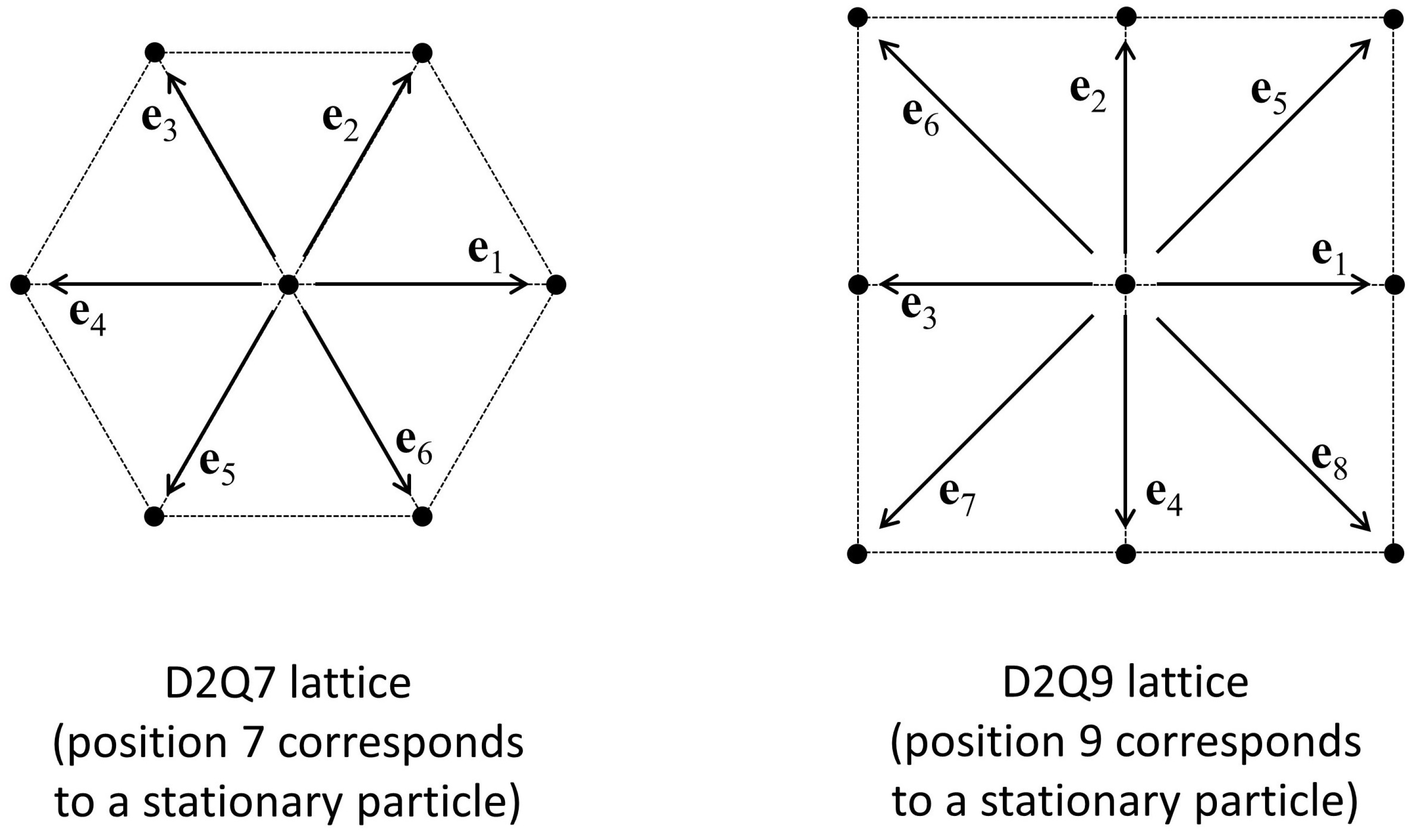
Figure 1 shows two possible lattice configurations that have been applied for modeling flow in two dimensions, along with the corresponding set of velocity vectors ${\mathbf{e}}_i$. These two configurations are commonly referred to as D2Q7 and D2Q9. The “D2” notation refers to the fact that the lattices are two-dimensional, and “Q7” or “Q9” refers to the number of neighbors for each node in the lattice (including the node itself as one of its neighbors, which allows for the possibility that a particle can remain stationary rather than moving to an adjoining node).

In classical statistical mechanics, $f(\mathbf{x},\mathbf{v},t)$ is the probability density function for fluid particles at location $\mathbf{x}$ having velocity $\mathbf{v}$ at time t. The Boltzmann equation for the movement of the fluid particles (in the absence of an external force field) is

$${\displaystyle \frac{\partial f}{\partial t}}+\mathbf{v}·\nabla f=\Omega$$

(3)

where $\Omega$ represents the change in particle momentum due to collisions. It can be seen that Equation (2) is a form of Equation (3) in which the time derivative has been discretized and in which the particle velocities are constrained to the lattice. Therefore, Equation (2) is sometimes termed the “lattice Boltzmann equation”.

A major advancement in the application of Equation (2) was developing a convenient way of estimating the collision operator. In classical statistical mechanics, Bhatnagar et al. [52] developed a method for estimating the collision operator in Equation (3); specifically, the collision operator is estimated as “relaxation” of the function f toward an equilibrium distribution $f^{\mathrm{eq}}$. The method of Bhatnagar et al. [52] was applied to the lattice Boltzmann equation by Qian et al. [53]. Qian et al. [53] presented the following equations, which constitute the very popular Bhatnagar–Gross–Krook (or “BGK”) formulation of the lattice Boltzmann method:

$$f_i(\mathbf{x}+{\mathbf{e}}_i\delta t,t+\delta t)=f_i(\mathbf{x},t)+{\displaystyle \frac{1}{\tau }}\left[f_i^{\mathrm{eq}}(\mathbf{x},t)-f_i(\mathbf{x},t)\right]$$

(4)

$$f_i^{\mathrm{eq}}(\mathbf{x},t)=w_i\rho \left[1+3({\mathbf{e}}_i·\mathbf{u})+{\displaystyle \frac{9}{2}}{({\mathbf{e}}_i·\mathbf{u})}^2-{\displaystyle \frac{3}{2}}(\mathbf{u}·\mathbf{u})\right]$$

(5)

where $\tau$ is a relaxation time characterizing the particle collision, $\rho$ is the fluid density (in the lattice domain), $\mathbf{u}$ is the macroscopic velocity vector of the fluid at location $\mathbf{x}$ and time t, and $w_i$ is a weighting parameter. Equation (5) is the formulation of $f^{\mathrm{eq}}$ that enables the macroscopic fluid behavior to adhere to the Navier–Stokes equations [53]. For this formulation, the viscosity of the fluid (in the lattice domain, units l.u.²/t.s.) is given by

$$\nu ={\displaystyle \frac{1}{6}}\left(2\tau -1\right).$$

(6)

The weighting parameters, $w_i$, depend on which lattice geometry is employed. For a D2Q9 lattice (shown in Figure 1), w is given by the following [53,54,55]:

$$w=\left[{\displaystyle \frac{1}{9}}{\displaystyle \frac{1}{9}}{\displaystyle \frac{1}{9}}{\displaystyle \frac{1}{9}}{\displaystyle \frac{1}{36}}{\displaystyle \frac{1}{36}}{\displaystyle \frac{1}{36}}{\displaystyle \frac{1}{36}}{\displaystyle \frac{4}{9}}\right].$$

(7)

For the flow of a fluid in two dimensions, the solution of Equations (4)–(7) enables us to track the particle distribution function f over time and space. However, Equation (5) depends on the macroscopic fluid properties $\rho$ and $\mathbf{u}$. These can be determined by calculating the moments of f, according to the following:

$$\rho (\mathbf{x},t)=\sum _i{f}_i(\mathbf{x},t)$$

(8)

$$\mathbf{u}(\mathbf{x},t)={\displaystyle \frac{{\sum }_i{f}_i(\mathbf{x},t){\mathbf{e}}_i}{{\sum }_i{f}_i(\mathbf{x},t)}}$$

(9)

Equations (4)–(9) constitute the foundation for simulating two-dimensional fluid flow with the lattice Boltzmann method. In practice, the method is implemented through an alternating series of “streaming” steps and “collision” steps that together satisfy Equation (4). More information about these steps is provided below in Section 3, but some details of implementation are omitted here in the interest of space. The reader is referred to previous work by Sukop and Thorne [6], Guo and Shu [43], Huang et al. [26], Krüger et al. [56], or Mohamad [57] for additional details of implementation.

It is worth noting that the LBM can also be used to simulate transport as well as fluid flow—for instance, mass transport via diffusion [58] and/or heat transfer via conduction [59]. Using the LBM to model transport rather than flow requires modification to the selection of the equilibrium distribution function $f^{\mathrm{eq}}$ and the relaxation time $\tau$ (e.g., [58,59]). However, in the present paper, we are concerned only with the multi-phase flow of immiscible fluids in porous media, and we do not consider diffusive mass transport or conductive heat transfer.

3. CGM Framework

The original CGM [25] was developed as a combination of the immiscible cellular gas automaton [24] and the LBM [50]. The method considers two immiscible fluids, a “red” fluid and a “blue” fluid, and thus considers two particle distribution functions $f^k$, where the superscript k indicates the red or the blue fluid. Particles of both fluids collide and stream in the lattice domain following the regular LBM operation described above (Section 2), but with an added “perturbation” step that enables interfacial tension to be included in the model, and with a “recoloring” step to maintain the fluids as immiscible.

Over the past three decades, the overall model algorithm has remained essentially unchanged, but improvements to the equations have resulted in better accuracy and better representations of true multi-phase fluid physics. Some early developments include increased capability to model fluids of unequal viscosity and/or density [60], improvement in the recoloring step [27], and modification of the perturbation equation [55]. These advances have enabled the model to be used for a wider range of fluid applications and have paved the way for developing three-dimensional models [42,61,62]. This section provides the framework of a two-dimensional CGM that includes the aforementioned improvements of Grunau et al. [60], Latva-Kokko and Rothman [27], and Reis and Phillips [55]. More recent updates pertinent to the contrast in fluid viscosity, calculation of the color gradient, and application of external forces are considered subsequently in Section 4, Section 5 and Section 6. Also, the extension of the two-dimensional CGM to three dimensions will be discussed in a future paper in this series.

The essence of the CGM can be expressed as the following analog to Equation (2) [62]:

$$f_i^k(\mathbf{x}+{\mathbf{e}}_i,t+1)=f_i^k(\mathbf{x},t)+{\Omega }_i^k(\mathbf{x},t)$$

(10)

where the collision operator ${\Omega }_i^k(\mathbf{x},t)$ now represents the aggregate of three steps: the single-phase collision ${\left({\Omega }_i^k\right)}^1$, the perturbation operation ${\left({\Omega }_i^k\right)}^2$, and a recoloring process. In practice, the order of the operations for implementing the CGM is as follows:

• Calculate macroscopic variables ${\rho }_{\mathrm{tot}}$, ${\rho }^k$, and $\mathbf{u}$;
• Calculate equilibrium distributions for red and blue fluids, $f^{\mathrm{eq},k}$;
• Apply the single-phase collision operator, ${\left({\Omega }_i^k\right)}^1$, for both fluids;
• Calculate the “color gradient” between red and blue fluids, $\mathbf{C}(\mathbf{x},t)$;
• Apply the perturbation operator, ${\left({\Omega }_i^k\right)}^2$, to account for interfacial tension;
• Perform a “re-coloring” step to maintain the immiscibility of fluids;
• Stream the particle distributions $f^k$.

These steps are discussed in more detail in the sub-sections following.

We note that there are variants in the CGM that do not exactly follow the sequence of steps listed above. For instance, one such variant [63,64,65,66] enables the whole algorithm to operate with any color distribution function. There can be advantages to such variants, including lower memory demands. However, in this review, we focus only on the more traditional CGM that relies on red and blue fluid populations, because of that method’s ubiquity and relative ease of implementation.

3.1. Calculation of Macroscopic Variables

The first step in the algorithm is the calculation of the macroscopic variables: the total density of the combined (composite) fluid ${\rho }_{\mathrm{tot}}$, the individual fluid densities ${\rho }^k$ for the red and blue fluids, and the velocity $\mathbf{u}$ of the combined fluid. Analogous to Equations (8) and (9), these macroscopic variables can be calculated from the moments of the red and blue distribution functions:

$${\rho }^k(\mathbf{x},t)=\sum _i{f}_i^k(\mathbf{x},t)$$

(11)

$${\rho }_{\mathrm{tot}}(\mathbf{x},t)=\sum _k{\rho }^k(\mathbf{x},t)$$

(12)

$$\mathbf{u}(\mathbf{x},t)={\displaystyle \frac{{\sum }_k{\sum }_i{\mathbf{e}}_i{f}_i^k(\mathbf{x},t)}{{\sum }_k{\sum }_i{f}_i^k(\mathbf{x},t)}}$$

(13)

3.2. Equilibrium Distribution Functions

The second step involves computing the equilibrium distribution functions $f^{\mathrm{eq},k}$ for the red and blue fluids, which are used subsequently (step 3) to calculate the single-phase collision operator [67,68]:

$$f_i^{\mathrm{eq},k}(\mathbf{x},t)={\rho }^k\left(C_i^k+w_i\left[3({\mathbf{e}}_i·\mathbf{u})+{\displaystyle \frac{9}{2}}{({\mathbf{e}}_i·\mathbf{u})}^2-{\displaystyle \frac{3}{2}}(\mathbf{u}·\mathbf{u})\right]\right)$$

(14)

For a D2Q9 lattice, $w_i$ in Equation (14) is given by Equation (7) and $C_i^k$ is given by the following [55,67]:

$$C_i^k=\left\{\begin{array}{cc}{\displaystyle \frac{1-{\alpha }^k}{5}}\hfill & \mathrm{if}i=1,2,3,4\hfill \\ {\displaystyle \frac{1-{\alpha }^k}{20}}\hfill & \mathrm{if}i=5,6,7,8\hfill \\ {\alpha }^k\hfill & \mathrm{if}i=9\hfill \end{array}\right.$$

(15)

In Equation (15), ${\alpha }^k$ is a parameter that introduces a density contrast between the fluids while maintaining stable hydrodynamic pressures at the interface (cf. [55,60]). The selected values of ${\alpha }^r$ and ${\alpha }^b$ determine the density ratio between the two fluids, the speed of sound within each fluid ($c_s^k$), and the pressure within the system, as summarized in

Table 1. User-specified CGM constants and their relations to fluid properties.

Symbol	Parameter	Fluid Relation
${\tau }^k$	Relaxation time of the $k\mathrm{th}$ fluid	Kinematic viscosity ${\nu }^k={\displaystyle \frac{1}{3}}({\tau }^k-0.5)$
${\alpha }^k$	Density parameter of the $k\mathrm{th}$ fluid	Density ratio of the two fluids $\gamma ={\displaystyle \frac{{\rho }^r}{{\rho }^b}}={\displaystyle \frac{1-{\alpha }^b}{1-{\alpha }^r}}$;
		speed of sound $c_s^k=\sqrt{\zeta (1-{\alpha }^k)}$;
		pressure $P^k={\rho }^k{\left(c_s^k\right)}^2={\rho }^k\zeta (1-{\alpha }^k)$
$A^k$	Interfacial tension constant of the $k\mathrm{th}$ fluid	Interfacial tension $\sigma$;
		see discussion in Section 3.5 regarding the
		relationship between $A^k$ and $\sigma$
$\beta$	Interface thickness parameter	See discussion in Section 3.6;
		$\beta \le 1$

. In Table 1, the parameter $\zeta$, which relates $c_s^k$ to ${\alpha }^k$, is lattice-dependent; values are provided by Leclaire et al. [69]. For a D2Q9 lattice, $\zeta ={\displaystyle \frac{3}{5}}$.

To simulate a stable density contrast, ${\alpha }^k$ must be selected within the range $0<{\alpha }^k<1$ for both fluids. In particular, for a D2Q9 lattice, if ${\alpha }^k=4/9$, Equation (14) reduces to Equation (5) for fluid k, and the speed of sound within fluid k is $c_s^k=1/\sqrt{3}$. For other values of ${\alpha }^k$, the speed of sound in fluid k will be different, as given in Table 1. To model the flow of two fluids of equal density, ${\alpha }^k$ for both fluids may usually be set equal to $4/9$. An introduction of different values of ${\alpha }^k$ for the two fluids is able to achieve density ratios up to about 18.5 [55]; systems with greater density ratios require a different approach, which will be reviewed in a subsequent paper in this series.

Note that to achieve a desired density ratio $\gamma$, there is not one unique pair of ${\alpha }^r$ and ${\alpha }^b$ that must be selected; for instance, selecting ${\alpha }^b=0.02$ and ${\alpha }^r=0.51$ will yield a density ratio $\gamma =2$, but selecting ${\alpha }^b=0.4$ and ${\alpha }^r=0.7$ will also yield $\gamma =2$. In limited trials during which we tested different combinations of ${\alpha }^r$ and ${\alpha }^b$, we found that setting both values of ${\alpha }^k$ close to $4/9$ led to slightly better results than allowing one value of ${\alpha }^k$ to be far from that value. The selection of ${\alpha }^r$ and ${\alpha }^b$ according to the equations shown in Table 1 ensures that the pressure in the two fluids is continuous at the fluid–fluid interface [55,67].

It has been demonstrated [66] that when using the aforementioned $f^{\mathrm{eq},k}$ relations for fluids of unequal density, the tangential momentum of the two fluids is conserved along the fluid–fluid interface, but the tangential velocity along the fluid–fluid interface then becomes discontinuous. It is not yet clear if there is a practical implication of conserving momentum rather than velocity during simulations, nor if a different method for modeling unequal densities would be able to ensure the continuity of tangential velocities [66].

3.3. Collision Operator

In the next step, the collision operator ${\left({\Omega }_i^k\right)}^1$ is computed and applied. There are different ways to compute the collision operator ${\left({\Omega }_i^k\right)}^1$ depending on the viscosity ratio of the two fluids. The simplest collision expression is the BGK formulation, which considers that collisions induce the “relaxation” of $f^k$ toward the equilibrium population $f^{\mathrm{eq},k}$, as discussed previously in Section 2:

$${\left({\Omega }_i^k\right)}^1={\displaystyle \frac{-1}{\tau }}\left[f_i^k(\mathbf{x},t)-f_i^{\mathrm{eq},k}(\mathbf{x},t)\right]$$

(16)

The challenge with applying Equation (16) is that it depends on a relaxation time $\tau$ that is related to the fluid viscosity (as shown in Equation (6)), but the fluid viscosity might not be the same for the red and blue fluids. If the red and blue fluids have a viscosity ratio that is very close to one (say, within a factor of two), then they will have similar values of $\tau$, and Equation (16) can be applied without difficulty. If the fluids have a viscosity contrast that is slightly less than ∼0.5 or slightly greater than ∼2, an “effective” viscosity can be computed by interpolation, as discussed subsequently in Section 4. For even greater viscosity contrasts, more sophisticated approaches are required; for instance, the BGK approach can be replaced by a multiple-relaxation-time (MRT) approach, which will be discussed in a subsequent paper in this series.

3.4. Computing the Color Gradient

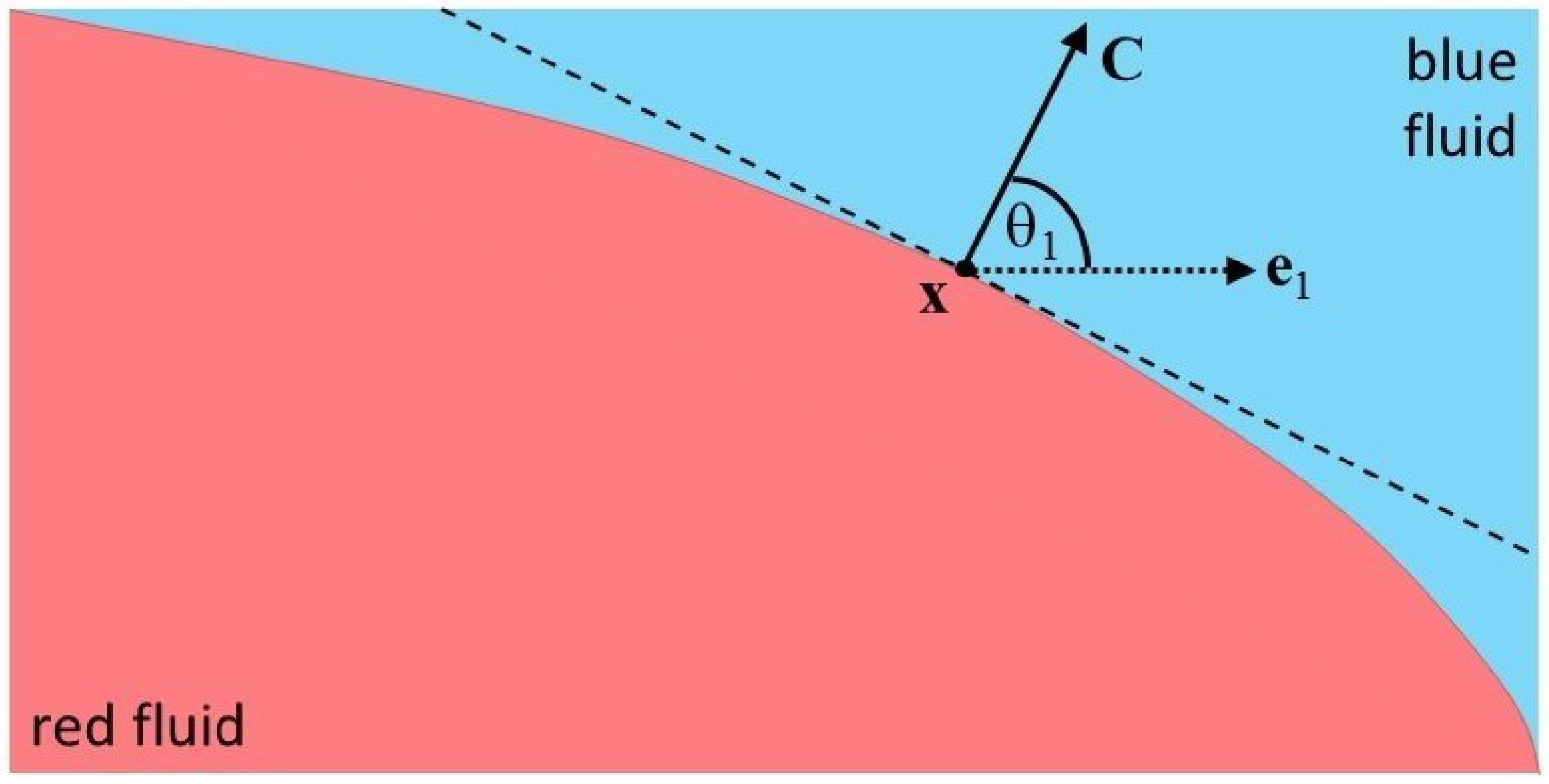
Next, the “color gradient” (sometimes also called “color flux” or “color field”), $\mathbf{C}(\mathbf{x},t)$, is calculated. The color gradient $\mathbf{C}(\mathbf{x},t)$ is the vector perpendicular to the interface between the red and blue fluids, as shown in Figure 2.

In the literature, different approaches have been presented for computing the color gradient. The original approach, as proposed and presented by Rothman and Keller [24], Gunstensen et al. [25], and Grunau et al. [60], is the following:

$$\mathbf{C}(\mathbf{x},t)=\sum _i{\mathbf{e}}_i\left[{\rho }^r(\mathbf{x}+{\mathbf{e}}_i,t)-{\rho }^b(\mathbf{x}+{\mathbf{e}}_i,t)\right]$$

(17)

Two notable modifications to this “original” approach are the “isotropic” color gradient of Leclaire et al. [70] and the “modified” color gradient of Xu et al. [71]. Subsequently in this paper (Section 5), we will compare some results of simulations using the original color gradient to the results of simulations using the isotropic color gradient of Leclaire et al. [70].

3.5. Perturbation

Gunstensen et al. [25] explain that the color gradient method proceeds by performing a collision step (as summarized above), then by “add[ing] a surface-tension-inducing perturbation”, then by recoloring the fluids and streaming the particles. In other words, the perturbation step of the CGM is the method of incorporating interfacial tension between the immiscible fluids; the color gradient $\mathbf{C}$ is utilized in this perturbation operation. In the paper of Gunstensen et al. [25], the perturbation step is represented by their Equation (17). Subsequently, perturbation strategies were proposed by Grunau et al. [60], Lishchuk et al. [72], Latva-Kokko and Rothman [27], and Reis and Phillips [55]. Ideally, the perturbation process should recover the correct interfacial force, reduce artificial velocities at the fluid–fluid interface (spurious velocities), retain the correct interface shape, and minimize interface thickness [62,72]. The approaches of Lishchuk et al. [72] and of Reis and Phillips [55] both fulfill these criteria. Furthermore, both methods have been applied successfully in both two-dimensional and three-dimensional models [42,62,72]. The approach of Lishchuk et al. [72] has been shown to model contact angles more accurately under certain conditions [45,73,74]. However, the approach of Reis and Phillips [55]—which is essentially an improvement upon the approaches of Grunau et al. [60] and Latva-Kokko and Rothman [27]—has been more extensively used because of its ability to include density ratios greater than one and because it is computationally less expensive. Here, we summarize the method of Reis and Phillips [55].

In this method, the perturbation step is accomplished through the application of the perturbation operator ${\left({\Omega }_i^k\right)}^2$ that is applied to each $f_i^k$:

$$f_i^k(\mathbf{x},t)=f_i^k(\mathbf{x},t)+{\left({\Omega }_i^k\right)}^2$$

(18)

$${\left({\Omega }_i^k\right)}^2={\displaystyle \frac{A^k}{2}}\left|\mathbf{C}\right|\left[w_i{\displaystyle \frac{{(\mathbf{C}·{\mathbf{e}}_i)}^2}{\mathbf{C}·\mathbf{C}}}-B_i\right]$$

(19)

where the parameter $A^k$ is a user-specified parameter (see Table 1) that controls the interfacial tension value. Equation (19) enables the conservation of mass and momentum, as explained by Reis and Phillips [55] and by Liu et al. [62]. In Equation (19), B is a vector of values that depends on the lattice employed; the proper selection of B enables the recovery of the correct interfacial force term in the Navier–Stokes equations [55,62]. Specifically, for a D2Q9 lattice:

$$B=\left[{\displaystyle \frac{2}{27}}{\displaystyle \frac{2}{27}}{\displaystyle \frac{2}{27}}{\displaystyle \frac{2}{27}}{\displaystyle \frac{5}{108}}{\displaystyle \frac{5}{108}}{\displaystyle \frac{5}{108}}{\displaystyle \frac{5}{108}}{\displaystyle \frac{-4}{27}}\right].$$

(20)

This method of introducing interfacial tension between the fluids has been shown to recover correct macroscopic equations for two-phase flows; detailed mathematical derivations are given by Reis and Phillips [55] and Liu et al. [62].

The interfacial tension between the two fluids, $\sigma$, is related to the $A^k$ parameters [27,60]. Either the user can specify the $A^k$ parameters, and the interfacial tension $\sigma$ will result from the choice of the $A^k$, or the user can specify the desired interfacial tension $\sigma$, and values of $A^k$ can be calculated accordingly. The problem is that the relationship between $A^k$ and interfacial tension has not been completely resolved; different papers give different derivations or approximations of the relationship. Also, the relation between $A^k$ and $\sigma$ is known to depend on the fluid viscosities and the associated collision relaxation times $\tau$; if the fluids have unequal viscosities, then they also have unequal values of $\tau$, which complicates the relation between $A^k$ and $\sigma$.

To simplify the situation somewhat, we found that, if the two fluids have equal densities or if the density ratio is acceptably low ($0.5\le \gamma \le 2.0$), a single value of A can often be used for both fluids, i.e., $A^r=A^b=A$. In this case, A can be computed from a desired value of $\sigma$ by following Equations (36) and (37) of Leclaire et al. [70]. That is, if the color gradient $\mathbf{C}$ is computed according to Equation (17), then A and $\sigma$ are related by

$$A={\displaystyle \frac{3}{4}}{\displaystyle \frac{\sigma }{({\rho }^r+{\rho }^b)\tau }}$$

(21)

in which $\tau$ is an interpolated or effective relaxation time, which will be explained subsequently in Section 4. If, instead of using Equation (17) to calculate $\mathbf{C}$, we instead use the isotropic color gradient of Leclaire et al. [70] (which will be discussed in more detail subsequently), then A must instead be computed by the following:

$$A={\displaystyle \frac{9}{2}}{\displaystyle \frac{\sigma }{({\rho }^r+{\rho }^b)\tau }}$$

(22)

in which, again, $\tau$ is an interpolated or effective relaxation time. Notably, because the interpolated relaxation time $\tau$ varies both spatially and temporally (as will be seen subsequently in this paper), the parameter A also varies spatially and temporally, so it must be computed at every lattice location at every time step.

If Equations (21) and (22) do not successfully produce the desired interfacial behavior, then alternatively, the interfacial tension $\sigma$ for selected values of $A^k$ can be verified or estimated by conducting a bubble test (static droplet test) and measuring the simulated pressures and droplet radius [62,68,75]. The perturbation term and its relationship to interfacial tension are also considered in more detail in Appendix A of Ginzburg and Steiner [63].

3.6. Recoloring

After the perturbation step, the fluids are still mixed and require separation. This is achieved by a “recoloring” step. The original recoloring procedure [25] suffered from numerical issues such as “lattice pinning” and fluctuations in velocity (also called “spurious currents” or “anomalous currents”) near the interface [27,76]. Subsequent recoloring algorithms proposed in the literature (e.g., [27,55,61,67]) were designed largely to address these numerical issues. The algorithm proposed by Latva-Kokko and Rothman [27]—which is an improvement to that of D’Ortona et al. [77]—has been found to perform well for a variety of tests and is presented here:

$$f_i^r(\mathbf{x},t)={\displaystyle \frac{{\rho }^r}{{\rho }_{\mathrm{tot}}}}{f}_i^{\mathrm{tot}}+\beta {\displaystyle \frac{{\rho }^r{\rho }^b}{{\left({\rho }_{\mathrm{tot}}\right)}^2}}cos\left({\Theta }_i\right)f_i^{\mathrm{eq},0}$$

(23)

$$f_i^b(\mathbf{x},t)={\displaystyle \frac{{\rho }^b}{{\rho }_{\mathrm{tot}}}}{f}_i^{\mathrm{tot}}-\beta {\displaystyle \frac{{\rho }^r{\rho }^b}{{\left({\rho }_{\mathrm{tot}}\right)}^2}}cos\left({\Theta }_i\right)f_i^{\mathrm{eq},0}$$

(24)

where $\beta$ is a user-specified parameter that controls the thickness of the interface (Table 1), and ${\rho }_{\mathrm{tot}}$ is the total fluid density as defined in Equation (12).

In Equations (23) and (24), $f_i^{\mathrm{tot}}(\mathbf{x},t)=f_i^r(\mathbf{x},t)+f_i^b(\mathbf{x},t)$ and $f_i^{\mathrm{eq},0}(\mathbf{x},t)$ are the equilibrium distribution function for the combined fluid under stationary conditions, i.e., evaluated at $\mathbf{u}=0$. For the calculation of $f_i^{\mathrm{eq},0}(\mathbf{x},t)$, we recommend using Equations (7), (14) and (15) given above, which differ slightly from Equations (1) and (2) of Latva-Kokko and Rothman [27]. Also, ${\Theta }_i$ represents the angle between the color gradient vector $\mathbf{C}$ and the lattice velocity vector ${\mathbf{e}}_i$, as shown in Figure 2 and given by the following equation:

$$cos(\Theta )={\displaystyle \frac{{\mathbf{e}}_i·\mathbf{C}}{|{\mathbf{e}}_i\left|\right|\mathbf{C}|}}$$

(25)

The parameter $\beta$ in Equations (23) and (24) is specified by the user and is set between 0 and 1. A $\beta$ value close to one gives minimum interface thickness but increases spurious velocities and reduces the accuracy of the interfacial tension value [62,68,78]. Conversely, if $\beta$ is set too low, the spurious velocities at the interface reduce, but the interface thickness increases. Usually, a value of $\beta$ between 0.70 and 0.99 is selected to maintain a thin interface without introducing significant spurious velocities (e.g., [79,80]), though Halliday et al. [78] argue that $\beta$ should not exceed $\sqrt{2}/2\approx 0.71$. Also, Leclaire et al. [81] offer a method for using a variable, rather than constant, value of $\beta$ to improve performance. Despite these subtleties, we generally found that a constant value of $\beta \approx 0.8$ works well as a “default” value, unless it is determined that a more sophisticated approach is required.

In the literature, alternatives to the recoloring procedure have also been proposed. A few of these have been reviewed briefly by Ginzburg [66]. For instance, Kehrwald [65] proposes an “anisotropic diffusion” algorithm as an alternative to recoloring, and demonstrates that the algorithm is able to reduce the spurious currents (anomalous currents) mentioned above. However, most implementations of the CGM still rely on the recoloring algorithm described above, perhaps because it is relatively simpler to implement.

3.7. Summary of Parameters Specified by Model User

To summarize, the parameters that must be specified by the model user are those listed in Table 1.

• We generally recommend $\beta =0.8$ as a default value for the interface thickness parameter $\beta$.
• For simulating fluids of equal density, we recommend ${\alpha }^r={\alpha }^b={\displaystyle \frac{4}{9}}$. For density ratios other than one, setting both values of ${\alpha }^k$ reasonably close to $4/9$ is recommended over setting one of the values far from $4/9$.
• For most applications, we recommend $A^r=A^b=A$, which can be calculated to produce a desired interfacial tension $\sigma$ as given by Equation (21) or (22). However, A must be calculated at each lattice node at each time step because of the temporal and spatial variability of the effective relaxation time $\tau$.
• Finally, the model user must specify either the relaxation time ${\tau }^k$ or the kinematic viscosity ${\nu }^k$ for each fluid, using Equation (6) to calculate whichever of the two was not specified explicitly.

4. Accounting for Fluids of (Moderately) Unequal Viscosity

The ratio of viscosity between the two fluids can strongly influence the overall behavior of the system. A classic example is “viscous fingering” that results from a less viscous fluid displacing a more viscous fluid in a porous medium [82,83]. The LBM is sometimes used as a tool to investigate and understand such mechanisms (e.g., [68,84,85,86]).

Although the CGM provides a robust framework to model multi-phase flow when the viscosity ratio is reasonably close to 1 (perhaps in the range 0.5–2), modifications to the methods of Section 3 are required if the viscosity ratio is far from 1. For instance, Rannou [87] demonstrated that the “standard” CGM could properly simulate two-phase flow in a channel for viscosity ratios as high as 10, but that simulated velocity profiles deviated from the correct values at higher viscosity ratios. This is because two fluids with unequal viscosities also have unequal values of $\tau$, the relaxation time in the BGK collision operator, according to Equation (6). Therefore, at the interface between the two fluids, $\tau$ is not clearly defined, which can lead to incorrect calculations in the vicinity of the interface [68,88].

To address this problem, an effective value of $\tau$ near the interface can be interpolated from the adjacent known ${\tau }^k$ values before the first collision operator ${\left({\Omega }_i^k\right)}^1$ is calculated. Methods available for interpolating $\tau$ have been presented by Grunau et al. [60], Tölke et al. [61], and Liu et al. [88], and are reviewed here.

In the method of Grunau et al. [60], an “order parameter” P (also sometimes called the “phase field” in the literature) can be calculated at any location $\mathbf{x}$ to indicate which of the two fluids, red or blue, dominantly occupies that location:

$$P(\mathbf{x},t)={\displaystyle \frac{{\rho }^r(\mathbf{x},t)-{\rho }^b(\mathbf{x},t)}{{\rho }^r(\mathbf{x},t)+{\rho }^b(\mathbf{x},t)}}$$

(26)

Values of P range from $-1$ (region is occupied only by the blue fluid) to $+1$ (region is occupied only by the red fluid). The value of $\tau$ at any location $\mathbf{x}$ near the interface is determined from P and a user-specified interface parameter, $\delta$, which must be $\le 1$:

$$\tau (\mathbf{x},t)=\left\{\begin{array}{cc}{\tau }^r\hfill & P>\delta \hfill \\ g^r\left(P\right)\hfill & \delta \ge P>0\hfill \\ g^b\left(P\right)\hfill & 0\ge P>-\delta \hfill \\ {\tau }^b\hfill & P<-\delta \hfill \end{array}\right.$$

(27)

$$\begin{array}{cc}\hfill g^r\left(P\right)& =s_1+s_{2}P+s_3{P}^2\hfill \\ \hfill g^b\left(P\right)& =t_1+t_{2}P+t_3{P}^2\hfill \\ \hfill s_1=t_1& =2{\displaystyle \frac{{\tau }^r{\tau }^b}{{\tau }^r+{\tau }^b}}\hfill \\ \hfill s_2& =2{\displaystyle \frac{{\tau }^r-s_1}{\delta }}\hfill \\ \hfill s_3& =-{\displaystyle \frac{s_2}{2\delta }}\hfill \\ \hfill t_2& =2{\displaystyle \frac{t_1-{\tau }^b}{\delta }}\hfill \\ \hfill t_3& =-{\displaystyle \frac{t_2}{2\delta }}\hfill \end{array}$$

(28)

Tölke et al. [61] use the same order parameter P as Grunau et al. [60], but the calculation of $\tau$ based on P is different. Specifically, Tölke et al. [61] use a simple linear interpolation to compute $\tau$ in the vicinity of the fluid–fluid interface:

$$\tau (\mathbf{x},t)={\displaystyle \frac{1}{2}}(1+P(\mathbf{x},t)){\tau }^r+{\displaystyle \frac{1}{2}}(1-P(\mathbf{x},t)){\tau }^b$$

(29)

Finally, the interpolation scheme of Liu et al. [88] is based on a method devised by Zu and He [89] for use in the free-energy method. This interpolation scheme again uses the same order parameter P, but now $\tau$ is evaluated as a weighted harmonic mean of ${\tau }^r$ and ${\tau }^b$:

$${\displaystyle \frac{1}{\tau (\mathbf{x},t)-0.5}}={\displaystyle \frac{1+P(\mathbf{x},t)}{2({\tau }^r-0.5)}}+{\displaystyle \frac{1-P(\mathbf{x},t)}{2({\tau }^b-0.5)}}$$

(30)

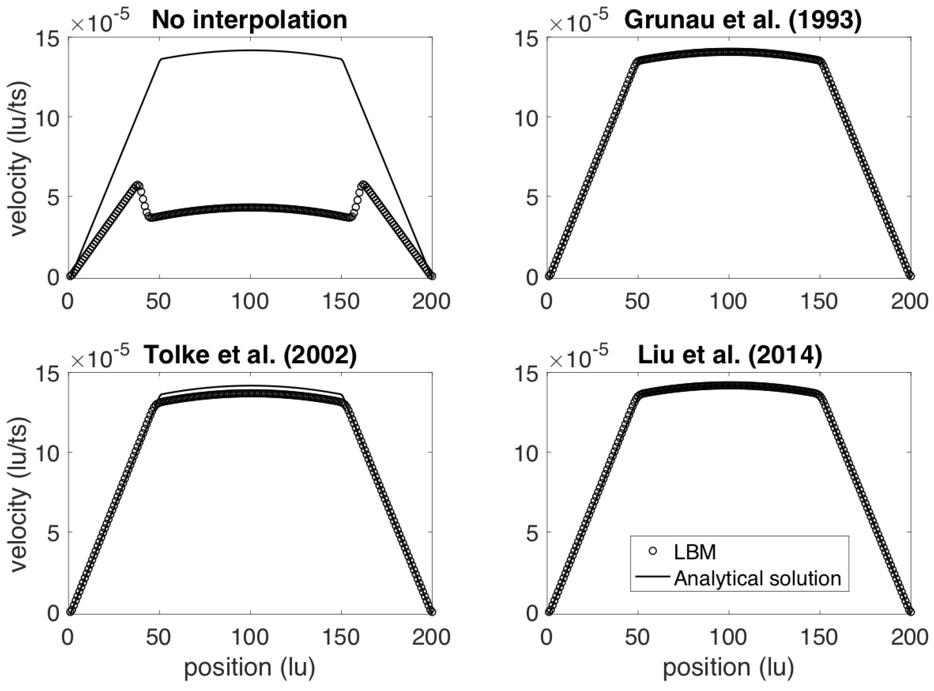
Figure 3 demonstrates the effectiveness of these three popular interpolation schemes for the classic benchmark simulation of two-phase flow in a channel (layered Poiseuille flow). For Figure 3, the testing domain is a $10\times 200$ lattice domain with periodic boundary conditions and with a force applied to the fluid in the middle of the channel (methods for applying a force to the fluid will be described subsequently in Section 6). Other details regarding the simulation parameters are provided by Liu et al. [88]. In this figure, we simulated the flow of two fluids with a viscosity ratio of $12.5$, i.e., the fluid in the middle of the channel (from lattice units 50 to 150) has a higher viscosity than that of the fluid near the edges of the channel. The CGM is used according to Section 3, and the LBM results are compared to a known analytical solution provided in Chapter 2 of Huang et al. [26] (cf., [32,40,87]). In Figure 3, we generated the results in the top-left panel without viscosity interpolation, and we generated the results in the remaining panels using the viscosity interpolation methods of Grunau et al. [60], Tölke et al. [61], and Liu et al. [88], as indicated on the figure. The improvement afforded by each viscosity interpolation is obvious.

All three interpolation schemes considerably reduce the error between the analytical and LBM velocities. Among these, the methods of Grunau et al. [60] and Liu et al. [88] perform similarly and accurately while the method of Tölke et al. [61] can not match the analytical solution completely. The methods of both Grunau et al. [60] and Liu et al. [88] have been successfully implemented and are popularly used [42,55,68,85,90]. The choice of which method to use is mostly up to the user’s preference, but we note that the method of Liu et al. [88] requires fewer computations without any apparent degradation of performance. We therefore use the method of Liu et al. [88] in any simulations discussed subsequently in this paper (Section 5 and Section 6).

In many applications, such as in simulations of drainage or imbibition, the fluid–fluid interface moves over time. Thus, the values of $P(\mathbf{x},t)$ change over space and time; so too then do the values of the interpolated viscosity $\tau (\mathbf{x},t)$. This means that any other variables that depend on $\tau$—for instance, A in Equations (21) and (22)—also change over space and time. The values of P, $\tau$, and A must therefore be recalculated at each lattice node at each time step.

As can be seen from Figure 3, the use of viscosity interpolation can, under some conditions, allow the CGM to perform well when the two fluids are of unequal viscosities. However, if the ratio of the fluid viscosities becomes extreme (e.g., the viscosity ratio is greater than ∼10), viscosity interpolation might not be sufficient to ensure that simulations are stable and accurate. Furthermore, the results observed in Figure 3 depend not only on the ratio of ${\nu }^r/{\nu }_b$ but also on the specific values of ${\nu }^r$ and ${\nu }^b$ selected; choosing different values of ${\nu }^r$ and ${\nu }^b$ might alter the results even if the ratio ${\nu }^r/{\nu }^b$ is held constant. BGK solutions are not necessarily fixed by non-dimensional numbers [66,91,92]. For either or both of these reasons, it might be necessary in some situations to employ more sophisticated approaches, such as replacing the BGK collision algorithm with a multiple relaxation time (MRT) algorithm. The application of the MRT to the color gradient method will be considered and reviewed in a future paper in this series.

When specifying values near an interface, as discussed immediately above, Ginzburg [66] distinguishes between an “implicit” interface approach (in which a blue fluid node is adjacent to a red fluid node, with an interface implied to exist halfway in between) and an “explicit” interface approach (in which a grid node is located at the interface, with blue fluid nodes on one side and red fluid nodes on the other side). For the case of an implicit interface, it is possible to select the CGM parameters in a way that the lattice Boltzmann method exactly reproduces the analytical solution for two-phase Poiseuille flow [66]. For the case of an explicit interface, Ginzburg [66] argues for using the harmonic mean value of viscosity, $\nu$, rather than relaxation time, $\tau$. This approach ensures the continuity of the tangential shear stress at the interface and the exact momentum solution inside each phase in two-phase Poiseuille flow, but needs to extrapolate it from the bulk to an explicit interface. Users may therefore wish to adopt the approach of Ginzburg [66] rather than interpolating values of $\tau$. Nevertheless, for relatively simple problems, interpolating the value of $\tau$ near the interface is an expedient way of accounting for moderate differences in fluid viscosities, as demonstrated by Figure 3.

5. Comparison of Two Methods for Computing the Color Gradient

In Section 3.4, we presented the original method of calculating the color gradient as proposed by Rothman and Keller [24], Gunstensen et al. [25], and Grunau et al. [60]. This method of calculating the color gradient has been used successfully in many applications (e.g., [29,55]). However, Leclaire et al. [70] noted that standard color gradient models (as described heretofore in this paper) are plagued by problems such as spurious fluid velocities near fluid interfaces and the inability to model fluids of widely varying densitities, and that these problems are due partly to the fact that the calculation of the color gradient (Equation (17)) contains discretization errors that are directionally biased (anisotropic). Leclaire et al. [70] therefore presented alternative ways of calculating the color gradient that remove the anisotropy of the discretization errors, which improves the accuracy and robustness of the model. We here refer to these as “isotropic” color gradient calculations, in contrast to the “original” color gradient calculation presented in Equation (17).

For a D2Q9 lattice, as shown in Figure 1, the following modification to Equation (17) can be used [70]:

$$\mathbf{C}(\mathbf{x},t)=\sum _i{\mathbf{e}}_i{\xi }_i\left[{\rho }^r(\mathbf{x}+{\mathbf{e}}_i,t)-{\rho }^b(\mathbf{x}+{\mathbf{e}}_i,t)\right]$$

(31)

in which the weights ${\xi }_i$ are given by the following:

$$\xi =\left[{\displaystyle \frac{1}{3}}{\displaystyle \frac{1}{3}}{\displaystyle \frac{1}{3}}{\displaystyle \frac{1}{3}}{\displaystyle \frac{1}{12}}{\displaystyle \frac{1}{12}}{\displaystyle \frac{1}{12}}{\displaystyle \frac{1}{12}}0\right].$$

(32)

For other lattice schemes (e.g., D3Q15 and D3Q27), the reader is referred to Leclaire et al. [70].

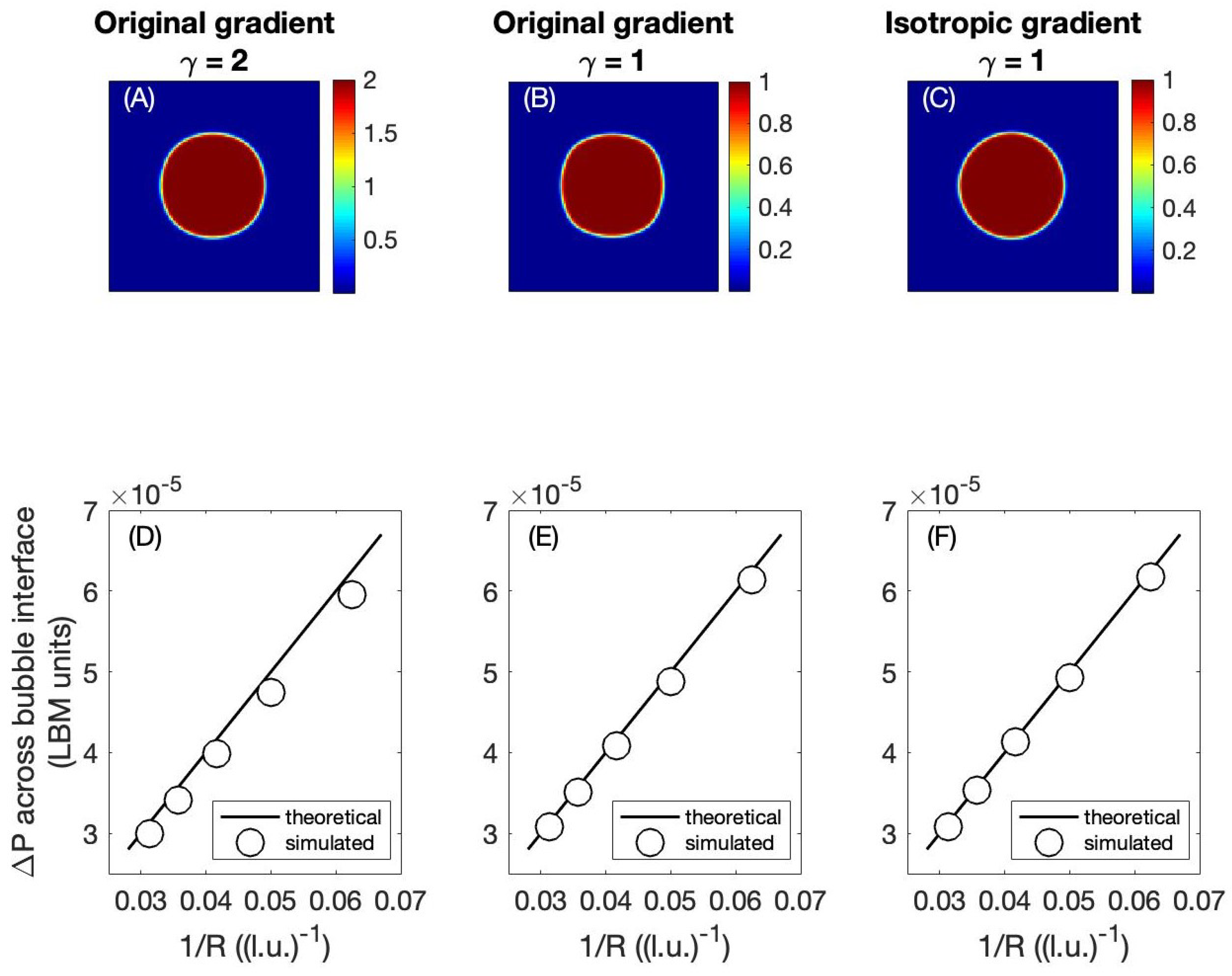
In Figure 4, we compare the original gradient approach to the isotropic gradient approach by applying both approaches to the problem of a “bubble test” or “droplet test”. For this test, a red fluid droplet of radius R is emplaced in a field of blue fluid, the system is allowed to equilibrate, and then the pressure drop is measured across the interface of the droplet. In two dimensions, the theoretical pressure drop across the interface is $\Delta P=\sigma /R$, where $\sigma$ is the interfacial tension specified by the user. The measured value of $\Delta P$ from the CGM simulation can be compared to the theoretical value of $\Delta P$ as a way to validate the CGM method. In Figure 4, the top row of panels shows the shape of the bubble after equilibration under different test conditions, and the bottom row of panels shows the agreement between measured and theoretical values of $\Delta P$ for those test conditions. For all simulations, the overall domain size was 128 × 128 l.u.; the specified interfacial tension was $\sigma =0.0010$ (in LBM units); the interface thickness parameter $\beta =0.85$; the viscosity ${\nu }^r={\nu }^b=0.16667$ l.u.²/t.s.; the simulations were allowed to equilibrate for 80,000 time steps before $\Delta P$ was measured; and the radius of the red droplet was varied between 16 and 32 l.u. (the top row of panels shows the results for the cases in which $R=32$ l.u.).

The left-most column in Figure 4 shows the results when ${\rho }^r=2.0$, ${\rho }^b=1.0$, and the original gradient is used. It can be seen that the droplet retains a mostly circular shape (panel (A)) and that the measured values of $\Delta P$ agree well with the theoretical relationship (panel (D)). A user might reasonably conclude that the original gradient calculation is acceptable for these test conditions. The center column of the figure shows the results when ${\rho }^r={\rho }^b=1.0$ and the original gradient is used. In this case, the measured values of $\Delta P$ are still close to the theoretical values (panel (E)), but the shape of the droplet is noticeably non-circular (anisotropic; panel (B)). The error in the gradient calculation is observable in the anisotropic shape of the droplet. Therefore, the right-most column of Figure 4 shows the results from the same conditions as the center column, but using the isotropic gradient calculation instead of the original gradient calculation. 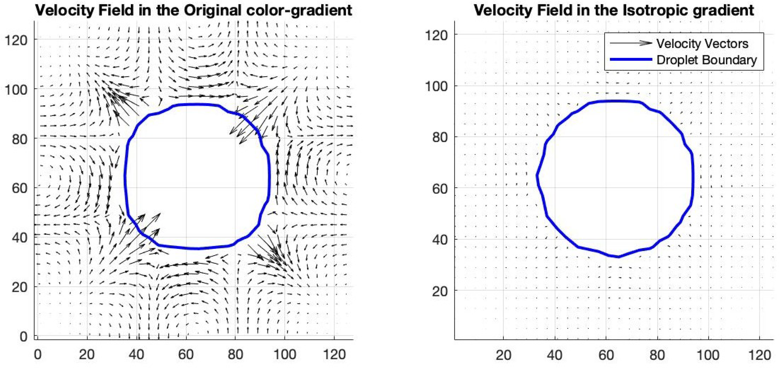The measured values of $\Delta P$ are slightly improved (panel (F)), and the droplet shape attains the desired circular shape (panel (C)). A comparison of panel (B) to panel (C) shows that the isotropic gradient is clearly preferable to the original gradient under these test conditions.

Moreover, there is a distinct difference in the generated spurious velocities in the original color gradient and the isotropic color gradient methods. For the test case shown in Figure 4 when R = 32 l.u., the maximum spurious velocities are equal to $2.3\times {10}^{-4}$ l.u./t.s. when using the original gradient calculation but are reduced to $7.1\times {10}^{-6}$ l.u./t.s. when the isotropic color gradient is used. These results are in agreement not only with the observations of Leclaire et al. [70] but also with those of Lafarge et al. [93] and Mora et al. [94]. The subject of spurious velocities in these simulations will be revisited in Section 7.

Therefore, in general, we recommend the isotropic gradient calculation (Equations (31) and (32)) over the original gradient calculation (Equation (17)). The simulation results are improved without any meaningful increase in the complexity or run time of the computer codes. However, when employing the isotropic color gradient, the user must be certain to use Equation (22) rather than Equation (21) when calculating the A parameter to yield a desired value of $\sigma$.

6. Application of a Force or Acceleration to the Fluids

A fluid flows in response to a pressure gradient or in response to a force acting on the fluid. Therefore, to simulate either single-phase or multi-phase flow, we must have methods for incorporating pressure gradients and/or external forces acting on the fluid(s). One way to do this is by specifying boundary conditions, e.g., specifying the fluid pressure or the fluid velocity on the boundaries of the domain [95]. Another approach is by including forces into the LBM simulations; methods that incorporate forces are often referred to as “forcing schemes” [56,96].

Many forcing schemes have been presented in the literature; a thorough review has been provided by Bawazeer et al. [96] for the flow of a single fluid. Here, we consider two of the most common forcing schemes and demonstrate how to apply them to a multi-phase flow simulation. In the first approach, originally proposed by Shan and Chen [20], external forces acting on the fluid are accounted for by including an acceleration term in the equilibrium distribution function $f^{\mathrm{eq}}$. In the second approach, proposed by Luo [97,98], a source term is added to include the force or acceleration as part of the collision step of the CGM.

In the method of Shan and Chen [20], the macroscopic velocity $\mathbf{u}$ in the computation of $f^{\mathrm{eq},k}$ is replaced by a new velocity ${\mathbf{u}}^{\mathrm{eq},k}$ that includes the effects of an acceleration ${\mathbf{a}}^k$ acting on fluid k. The acceleration ${\mathbf{a}}^k$ need not necessarily be the same on the red fluid and the blue fluid. Thus, Equation (14) becomes

$$f_i^{\mathrm{eq},k}(\mathbf{x},t)={\rho }^k\left(C_i^k+w_i\left[3\left({\mathbf{e}}_i·{\mathbf{u}}^{\mathrm{eq},k}\right)+{\displaystyle \frac{9}{2}}{\left({\mathbf{e}}_i·{\mathbf{u}}^{\mathrm{eq},k}\right)}^2-{\displaystyle \frac{3}{2}}\left({\mathbf{u}}^{\mathrm{eq},k}·{\mathbf{u}}^{\mathrm{eq},k}\right)\right]\right)$$

(33)

in which

$${\mathbf{u}}^{\mathrm{eq},k}(\mathbf{x},t)=\mathbf{u}(\mathbf{x},t)+{\mathbf{a}}^k\tau$$

(34)

and $\tau$ represents the interpolated relaxation time at location $\mathbf{x}$ and time t. The remainder of the color gradient algorithm remains unchanged. Thus, in practice, only the calculation of $f^{\mathrm{eq},k}$ needs to be changed to implement this forcing scheme.

The method of Luo [97,98] accounts for forces in a different manner than the method of Shan and Chen [20]. Here, the macroscopic velocity $\mathbf{u}$ and the calculation of $f^{\mathrm{eq},k}$ remain unchanged, i.e., Equation (14) is used as presented. To account for the acceleration ${\mathbf{a}}^k$ acting on the fluids, a source term $S_i^k$ is calculated as:

$$S_i^k(\mathbf{x},t)=w_i{\displaystyle \frac{{\rho }^k(\mathbf{x},t)}{{\left(c_s^k\right)}^2}}\left({\mathbf{e}}_i·{\mathbf{a}}^k\right)$$

(35)

in which $w_i$ is given by Equation (7). The source term $S_i^k$ must be calculated for both fluids at each location $\mathbf{x}$, each time t, and for each of the nine directions. As with the method of Shan and Chen [20], the method of Luo [97,98] allows for a different acceleration acting on the red and blue fluids. The source term is then incorporated into the collision step as follows:

$$f_i^k(\mathbf{x}+{\mathbf{e}}_i,t+1)=f_i^k(\mathbf{x},t)+{\left({\Omega }_i^k\right)}^1+S_i^k(\mathbf{x},t)$$

(36)

in which ${\left({\Omega }_i^k\right)}^1$ is given by Equation (16) assuming that the BGK algorithm is used.

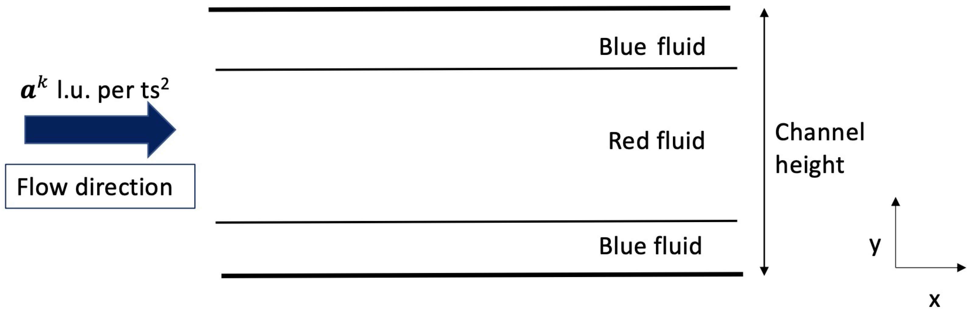
We compared the two forcing schemes described above via a layered Poiseuille flow validation test. In this test, red and blue fluids both flow between two parallel plates. A layer of red fluid is “sandwiched” in the middle of the channel between two layers of blue fluid. An acceleration a is applied in the $+x$ direction to the red fluid only, which induces flow. The situation is depicted graphically in Figure 5. This is a classic validation test for simulations of multi-phase flow because there is an analytical solution for the resulting velocity profile in the channel; see, for instance, Liu et al. [88].

We performed the test using a domain of 10 nodes in the x-direction and 120 nodes in the y-direction. As shown in Figure 5, the top and bottom walls are solid boundaries at which a no-slip boundary condition (half-way bounceback) is imposed. Periodic boundary conditions are applied on the left and right boundaries, which is why only 10 nodes are required in the x-direction. We performed the test for both the Shan and Chen [20] forcing scheme, which we now call the “feq-accel” method following Bawazeer et al. [96], and the Luo [97,98] forcing scheme, which we now call the “source term” method. For both methods, we tested viscosity ratios (${\nu }^r/{\nu }^b$) of 0.25 and 4.0; thus, a total of four simulations were performed. For all tests, the interfacial tension $\sigma =0.010$, the applied acceleration on the red fluid was $a^r=1.5\times {10}^{-8}$ l.u./(t.s.)², the interface thickness parameter $\beta =0.9$, the fluid densities ${\rho }^r={\rho }^b=1.0$, and simulations were run for at least 80,000 time steps to ensure that steady state was reached.

The results of the simulations are shown in Figure 6. The figure shows the velocity profiles of the fluids between the two parallel plates. At the top and bottom of the domain (i.e., at the two plates), the fluid velocity is 0 because of the no-slip boundary condition. The velocity reaches a maximum in the middle of the channel. There are two key findings as illustrated in Figure 6: first, there is no noticeable difference between the the left two panels [20] and the right two panels [97,98] of the figure, indicating that the two forcing schemes yield indistinguishable results for this test problem; second, both methods yield results that agree nearly perfectly with the analytical solution, indicating that either method is acceptable for the conditions tested.

The equivalence of the two forcing schemes in Figure 6 is not surprising for the particular test problem considered. An examination of Equations (10), (14), (16) and (33)–(36) shows that the two methods are mathematically equivalent for cases in which the last two terms of the $f^{\mathrm{eq}}$ distribution functions can be ignored. This is the case for grid-aligned Poiseuille flow; see Ginzburg et al. [91]. Also, the relationship and agreement between these two methods for the case of single-fluid flow have been elucidated by Huang et al. [99].

Based on the agreement between the two methods, it is not the case that one method is generally “better” than the other for multi-phase flow simulations that use the BGK collision operator. Nevertheless, we find it useful to present and compare the two proposed approaches here, for a few reasons. First, some previous papers have indicated that using gravitational acceleration in multi-phase simulations is not preferred (e.g., [19,75]), which points toward the use of an “external” forcing scheme. Second, Silva [100] demonstrated that if the applied force is spatially varying, including the acceleration term in the $f^{\mathrm{eq}}$ expression leads to a discrepancy between the CGM and the incompressible Navier–Stokes equations with an external body force under steady-state conditions; this also argues in favor of the source term forcing scheme. Finally, we found that when deploying more advanced CGM techniques, such as multiple relaxation times instead of the BGK collision scheme, one or the other of these two proposed forcing schemes can sometimes be easier to implement or code in practice. It is therefore useful to the reader to be familiar with both approaches in case a particular problem favors one over the other from a practical standpoint.

7. Challenges of Simulating Multi-Phase Flow in CGM

A multi-phase simulation in the CGM must be free from artificial fluid effects, which can arise near fluid–fluid and fluid–solid boundaries. For example, a good multi-phase simulation involves distinct phases separated by a thin interface, maintains fluid continuity between the phases, provides minimal fictitious or spurious velocities, and provides minimal fluid distortion. Therefore, a main challenge in the CGM is accurately depicting fluid flow while eliminating any artificial fluid effects. There is no numerical multi-phase flow model that is 100% accurate and free from error. However, by understanding the principles and theoretical foundations of the CGM, such errors can be minimized, and the method can provide a reasonable depiction of fluid flow processes.

One common error in the CGM is the presence of spurious velocities, i.e., the presence of fictitious fluid velocities where the fluids are supposed to be stationary. Such spurious velocities can arise near the interface of a bubble or droplet, as in Section 5. In that section, we discussed how the calculation of the color gradient can influence the droplet shape, as shown in Figure 4. The calculation of the color gradient can also affect the magnitude of spurious velocities. The algorithms discussed heretofore in this paper have made efforts to reduce or eliminate those fictitious velocities, but they usually do not disappear completely [68,70,94]. Specifically, for the case shown in Figure 4, the maximum magnitude of these spurious velocities is around $2.3\times {10}^{-4}$ l.u./t.s. when using the “original” color gradient and around $7.1\times {10}^{-6}$ l.u./t.s. when using the isotropic color gradient; see Figure 7. By using a higher-order gradient discretization, artificial velocities can be reduced, which also accompanies a reduction in the distortion in fluid shape (as seen in Figure 4).

In a CGM simulation, the major challenges are minimizing the presence of spurious velocities, ensuring pressure continuity between phases, minimizing the interface thickness, and minimizing distortion in fluid shape (e.g., droplet shape). This paper focused on the BGK-CGM formulation, and errors were considered in the context of common CGM code-validation tests that can be implemented with the BGK collision algorithm—which means that we considered relatively “easy” test conditions. In cases where simulations must account for fluid wettability, a higher viscosity ratio, and/or a higher density ratio, errors are likely to become more prominent. In future papers in this series, we will review efforts that have been made to minimize errors in more sophisticated contexts [87,101,102].

Another challenge in executing the LBM simulations—not limited to the color gradient method—is appropriately determining the relationship between “LBM variables” and “real-world variables”. This is achieved by using appropriate unit conversions for length, time, and mass. For instance, what real-world length scale is represented by one lattice unit, and what real-world time scale is represented by one time step? The concepts of scaling the LBM units have been considered previously by Pan et al. [5], Krüger et al. [56], and Baakeem et al. [103], among others. A key point is that, in many instances, particularly if we want to model the flow of low-viscosity fluids, the LBM lattice unit and time step must correspond to very small values of real-world length and time—millimeters and milliseconds, or perhaps even smaller. Thus, a simulation that takes hours to run might only simulate, say, the fluid flow through a 10 cm × 10 cm square for a period of a few minutes. Therefore, modeling fluid flow through large domains (a scale of meters) over time scales of hours or days can be very computationally expensive. A way to address the challenge of computational expense is through the parallelization of the LBM algorithms, which has been considered elsewhere [12,15,18,19,104].

8. Summary and Conclusions

Over the past 30 years, the lattice Boltzmann method (LBM) has become increasingly popular for modeling multi-phase fluid flow in porous media, and one popular variant of the LBM is the color gradient method. However, along with the rising popularity of the color gradient method has come a proliferation of different proposed algorithms and strategies for implementing various aspects of the method. Selecting the “best” algorithms and subroutines is daunting, especially for relatively new users of the method. Therefore, we aim to critically review the capabilities and implementation of the CGM, particularly for modeling pore-scale multi-phase flow in porous media, through a series of papers, of which this is the first.

In this paper, we provided a brief introduction to the LBM and CGM that enables and facilitates consideration of the subsequent topics. Following that introduction, we reviewed three specific aspects of color gradient modeling: different methods for modeling the flow of fluids of moderately different viscosities, different methods for calculating the color gradient, and different methods for modeling external forces or accelerations acting upon the flowing fluids. Specific findings from this paper include the following:

• Spatial interpolation of the collision relaxation times, $\tau$, enables accurate modeling of the flow of fluids of different viscosities as long as the viscosity contrast is moderate;
• Of the methods considered for $\tau$ interpolation, that of Liu et al. [88] is accurate and easy to implement;
• Using the “original” color gradient calculation of Rothman and Keller [24], Gunstensen et al. [25], and Grunau et al. [60] is sufficient in some cases, but the “isotropic” color gradient calculation of Leclaire et al. [70] improves upon the original method without any significant increase in model complexity;
• External accelerations acting on the flowing fluids can be modeled using a variety of forcing schemes, but for simple problems, there is no significant difference between the “feq-accel” forcing scheme of Shan and Chen [20] and the “source term” forcing scheme of Luo [97,98].

Understanding these aspects of the color gradient method is necessary and sufficient to allow the user to perform two common “benchmark” tests of lattice Boltzmann modeling, namely bubble tests and layered Poiseuille flow.

Future papers in the series will build upon these topics, considering phenomena or conditions such as fluids of widely differing viscosity and/or density, how to introduce the “wettability” of solid surfaces and specify a desired contact angle, how to simulate fluid flow in a domain with an open boundary condition (e.g., fluid flushing out of a porous medium), and how to extend the CGM from two spatial dimensions to three. By systematically reviewing these key aspects and features, this series of papers will extend our collective ability to apply the CGM to a variety of important problems in geosciences and engineering.