Investigation of Multiphase Flow in Continuous-Casting Water Model with Measurements and Computational Modeling

Abstract

This work introduces a 0.6-scale water model of the continuous slab-casting process and a MATLAB-based model to study the effects of non-primed and multiphase flow on pressure and flow rate. The water model uses stopper-rod flow control and features pressure and velocity measurements at multiple locations. The new computational model, PFSR V4 (Pressure-drop Flow-rate model of Stopper Rod metal delivery systems, Version 4), improves upon a prior one-dimensional Bernoulli-based framework by incorporating a bubble accumulation zone. This zone represents a region of bubbly flow with an intermediate gas fraction between constant-pressure gas pockets below the stopper tip and the downstream bubbly flow regime. Parametric studies with the water model show that flow remains fully primed at low gas flow rates but transitions to non-primed flow as the gas flow rate exceeds 10–16 SLPM. Three different flow regions are observed inside the water model nozzle: air pocket, bubble accumulation, and bubbly flow, which are also captured by the new computational model. Above a critical gas flow rate, the flow becomes unstable and difficult to control, though higher hot gas flow rates are expected for similar transitions in a real steel caster due to gas expansion at high temperatures. Pressure changes are minimal in the air pocket region and increase significantly in the upper bubble accumulation zone, where liquid velocity is much higher than in the classic bubbly-flow region, found lower in the nozzle. The new model was successfully calibrated to match the observed flow regimes and shows good agreement with the water-model measurements.

1. Introduction

Multiphase flow involves the simultaneous flow of two or more phases of gas, liquid, or solid [1]. Multiphase flow involving significant fractions of liquid and gas is encountered in numerous industrial applications, such as boiling and condensation processes [2,3], aerosol flows in the environment [4,5], natural gas and petroleum flows [6], nanofluids [7], processing and refining of molten metals, including aluminum [8] and, most importantly for this study, steel [9]. Such multiphase flows inside a pipe can experience many different flow regimes, including stratified smooth and wavy flows [6,10,11,12], plug flow [13,14,15,16,17], slug flow [18,19,20,21,22], annular flow [23,24,25,26] and bubbly flow [27,28,29,30,31].

Numerous experimental investigations into two-phase liquid–gas multiphase flows during molten metal processing have been conducted [32,33,34,35,36,37,38,39,40]. In the continuous casting of steel, liquid metal/gas flow has been investigated in several laboratory-scale models using analogue liquid metals for molten steel [35,36,37,38,39,40]. Terzija et al. [35,36] studied such flows in a 1:10-scale model of a commercial caster utilizing the eutectic liquid alloy GaInSn, owing to its similar properties to molten steel, including viscosity, surface tension, and electrical conductivity. Argon gas was injected through the stopper-rod tip, and the two-phase metal/argon flow behavior was observed, including the influence of electromagnetic braking systems. A novel inductive sensor array was implemented to measure the flow velocities. Periodic oscillation patterns were observed, which make the argon gas distinguishable from the main liquid phase and is more evident with increasing gas injection.

Eckert et al. [37] explored improved contactless measurement techniques for liquid metal flows by studying channel flows with liquid sodium or lead. These include ultrasound Doppler velocimetry and contactless magnetic tomography, which are used to quantify the internal velocity distribution. Timmel et al. [38] and Gerbeth and Eckert [39] investigated electromagnetic effects on multiphase flow patterns in the steel continuous-casting mold region using a tin–bismuth alloy (Sn60Bi40) and the eutectic alloy GaInSn. This included the Submerged Entry Nozzle (SEN) or stopper-rod metal delivery system.

Recently, Timmel et al. [40] used X-ray imaging to investigate two-phase flow regimes in a vertical pipe, with a downward flow of molten GaInSn and horizontal argon gas injection through the wall. Electromagnetic stirring was observed to induce swirling flow, directing the heavy liquid metal outward and driving the gas inward, promoting uniform bubble distribution. Without stirring, gas accumulates near the walls. Increasing stirring transitions the flow through three regimes: a twisted wall void zone, a central void zone, and a central bubble chain.

Computational models have been used extensively to study multiphase flow in continuous steel casters and physical laboratory models [41,42,43,44,45,46,47,48,49,50,51,52]. These include the effect of clogging on flow in the continuous casting of steel [41,43], flow in the nozzle [42,43,44,45,53], and mold/strand [54,55,56]. This is summarized in prior reviews [57,58]. Most previous models use computational fluid dynamics (CFD) methods, where partial differential equations for mass and momentum balance are solved using finite-difference, finite-volume, or finite-element methods, which discretize the three-dimensional domain into small volumes [44,45]. Recently, a simpler Bernoulli-based energy-balance approach has been applied, using a one-dimensional (1-D) discretization in the flow direction [41,42,43].

Bai and Thomas [46] demonstrated that pressure drops extensively just below the flow restriction caused by the stopper or slide gate and usually falls below atmospheric pressure. This negative gauge pressure is problematic because any air aspiration through cracks or joints in the refractories causes reoxidation inside the nozzle, leading to nozzle clogging and inclusion quality problems in the product. Argon gas injection is able to raise the pressure, in part by taking space, which requires the opening to increase and lessen the flow restriction. However, the argon flow rates needed to completely alleviate the negative pressure problem are usually excessive.

Liu et al. [43] applied a Bernoulli-based model to quantify how increasing clogging requires greater stopper-rod openings to maintain a constant flow rate. Yang et al. [47] further refined this methodology to analyze pressure distribution in slide-gate systems and show that reducing submerged entry nozzle (SEN) diameter at a given casting speed and gas flow rate enables larger openings, lessening the negative pressure problem.

Javurek et al. [48,49] introduced a Bernoulli-based model with empirical loss coefficients for single-phase and multiphase flows, offering pressure predictions across the system. Eck [50] proposed a similar model with a user-friendly graphical user interface (GUI), emphasizing single-phase flow in stopper-rod systems with a single-tip radius.

Only a few previous computational models have investigated pressure distributions within steel continuous-casting systems [34,35,36,37,49,50,51] with slide-gate [44,45,46,47,59,60] or stopper-rod [60,61] flow-control systems. Bai et al. [53] modeled the flow of argon gas through the tundish nozzle refractory, including the effect of thermal expansion and pressure changes. Recently, Olia et al. [51,52] developed two Bernoulli-based models in MATLAB v2022a to calculate the pressure and flow rate distributions during continuous-casting of steel in slide-gate (PFSG) and stopper-rod (PFSR) flow control systems. Both programs are versatile and computationally efficient modeling packages that include user-friendly graphical interfaces and inverse-modeling solvers. They account for argon gas injection with gas volume expansion based on the local pressure, three-radius stopper-rod tip geometries, and spatially variable clogging within the nozzle. Although they are 1-D models, they were successfully verified against full 3-D CFD simulations. The PFSR model introduces the effects of cavitation and non-primed flow, which can overcome issues with excessive negative gauge pressure predicted with conventional models in steel casters [52].

2. Previous Water Modeling

Many water model experiments have been conducted to better understand multiphase flow in real steel continuous casting [61,62,63,64,65,66]. These physical models enable easy visualization of the flow pattern and measurements such as pressure, velocity, and temperature. However, to capture flow in a caster with a water model, major differences must be overcome. First, the important differences in fluid properties, such as density, viscosity, surface tension, and multiphase contact angle, must be considered. The top surface is often open to the atmosphere, whereas the real caster is covered with mold slag. Most importantly, the water model lacks shell solidification; thus, the liquid flow volume is different [54]. The water model has a bottom, delivering flow to a return reservoir and pump, while the liquid domain of the steel caster decreases gradually. If the water model is not long enough, flow in the mold can be altered by a deflection off of the bottom [67]. Only flow in the mold can be studied because deeper in the caster, buoyancy forces due to temperature variations and solutal density differences become significant relative to the small inertial forces [68].

Many water models are constructed at full scale, which enables the use of real plant parts (such as nozzles) and also facilitates easy operating training. To lower construction costs, space requirements, operating costs, and other complexities, water models often have reduced scale. Thus, several parameters should be considered when constructing a water model to match the flow pattern in a real caster. These include characteristic length L [m], velocity V [m/s], density $\rho$ [kg/m³], dynamic viscosity $\mu$ [Pa·s], surface tension $\sigma$ [N/m], and contact angle with other phases $\theta$. Of course, the density and dynamic viscosity can be reduced to the single parameter of kinematic viscosity $\upsilon$ [m²/s].

To ensure that flow is the same in the water model and steel caster, the dimensionless groups that govern the relevant forces should match. As follows, these include the Reynolds number, Froude number, and also Weber number if the multiphase flow is involved:

$$Re={\displaystyle \frac{\rho VL}{\mu }}={\displaystyle \frac{VL}{\upsilon }}={\displaystyle \frac{\mathrm{Inertial} \mathrm{Force}}{\mathrm{Viscous} \mathrm{Force}}}$$

(1)

$$Fr={\displaystyle \frac{V^2}{gL}}={\displaystyle \frac{\mathrm{Inertial} \mathrm{Force}}{\mathrm{Gravitational} \mathrm{Force}}}$$

(2)

$$We={\displaystyle \frac{\rho V^{2}L}{\sigma }}={\displaystyle \frac{\mathrm{Inertial} \mathrm{Force}}{\mathrm{Surface} \mathrm{Tension} \mathrm{Force}}}$$

(3)

where $g$ is gravitational acceleration [9.81 m/s²]. It is important to note that at 25 °C, the kinematic viscosity of water is almost the same as that of molten steel. Simultaneous Re and Fr similarity can be achieved with a full-scale water model. Previous work has shown that achieving Re similarity may not be required if the flow is fully turbulent [54]. In multiphase flow, it is more important to satisfy We and Fr number similarity, which can be achieved by careful choice of the scale factor, $\lambda$ [54], as follows:

$$\lambda ={\displaystyle \frac{L_w}{L_s}}$$

(4)

• First, setting the Froude numbers of the water model (subscript w) and actual steel caster (subscript s) to be equal gives the following:

  $${\left({\displaystyle \frac{V^2}{gL}}\right)}_w={\left({\displaystyle \frac{V^2}{gL}}\right)}_S$$

  (5)
• Canceling the gravity constant and rearranging Equations (4) and (5) gives the following relationship between the scale factor and the flow speed ratio:

  $$\lambda ={\left({\displaystyle \frac{V_w}{V_s}}\right)}^2$$

  (6)
• Next, setting the Weber numbers equal and rearranging Equations (4) and (6) gives another following relationship between the scale factor and the velocity ratio:

  $$\lambda ={\displaystyle \frac{{\rho }_s}{{\rho }_w}}{\displaystyle \frac{{\sigma }_w}{{\sigma }_s}}{\left({\displaystyle \frac{V_s}{V_w}}\right)}^2$$

  (7)
• Solving Equations (6) and (7) for $\lambda$ gives the following:

  $$\lambda =\sqrt{{\displaystyle \frac{{\rho }_s}{{\rho }_w}}{\displaystyle \frac{{\sigma }_w}{{\sigma }_s}}}$$

  (8)
• Finally, inserting typical values of density and liquid–gas surface tension (${\rho }_s$ = 7020 kg/m³, ${\sigma }_s$ = 1.6 N/m, ${\rho }_w$ = 998 kg/m³, ${\sigma }_w$ = 0.073 N/m) gives the following [54]:

  $$\lambda \approx 0.6$$

  (9)

Based on the above calculations, simultaneous We–Fr similarity can be achieved with a 0.6-scale water model. Inserting this value into Equation (6), the velocities of the molten steel and water systems are related by the following:

$$V_s={\lambda }^{-0.5} V_w$$

(10)

The corresponding gas flow rates in the full-scale steel caster are more difficult to estimate. Aiming to match the flow behavior inside the nozzle, the gas flow rate in the water model should correspond to the hot gas flow rate in the steel caster. Further assuming the same hot gas fraction inside the nozzle for both the water model and steel caster using Equation (28) in Section 4.2, the injected flow rate of air in the water model, $Q_{air}$, can be used to estimate the corresponding hot flow rate of argon gas in the steel caster, $Q_{ar}$, by the following:

$$Q_{ar}={\displaystyle \frac{Q_{air}{Q}_s}{Q_w}}=Q_{air}{\displaystyle \frac{V_s}{V_w}}{\displaystyle \frac{A_s}{A_w}}=Q_{air}{\lambda }^{-2.5}$$

(11)

where $Q_s$ and $Q_w$ are the liquid flow rates (LPM) of steel and water, which are calculated from the velocities ($V_s$ and $V_w$), knowing the corresponding cross-sectional areas ($A_s$ and $A_w$), and taking into account the effect of $\lambda$ on those areas (which is proportional to the square of $\lambda$, based on Equation (4)). The cold gas flow rate, reported at standard conditions in SLPM, is naturally the same as the hot gas flow rate in the water model; hence, this is not considered in the evaluation of the current results. This is because, in the steel caster, the cold gas flow rate is ~5× smaller, owing to its lower temperature and higher pressure relative to the hot gas. This value and the corresponding cold argon flow rate are calculated using Equation (29), which is presented and discussed in Section 4.2.

However, even with fully turbulent flow and matching Fr and We (the above 0.6 scale model), the multiphase flow in a water model still differs from that in the corresponding steel caster [69,70], especially when slag is involved [67,70]. This is because multiphase flow phenomena are very complex, involving slag–steel interaction, bubble size distribution, slag/steel viscosities, slag/steel densities, slag/steel surface tensions, interfacial slag/steel/gas/refractory contact angles, bubble breakup and coalescence, droplet emulsification, bubble and droplet coalescence, and many other phenomena.

The aim of this paper is to better understand multiphase flow, pressure drop and velocity relations in continuous-casting nozzles using both physical water model experiments and a new Bernoulli-type mathematical model. This is accomplished by (1) observing the flow regimes and measuring pressure drop and velocity vs. vertical distance and (2) modeling the corresponding flow regions, pressure drops and velocities. The new model extends our previous PFSR model, which was already verified with CFD simulations and validated with measurements in previous work [52].

3. Current Water Model

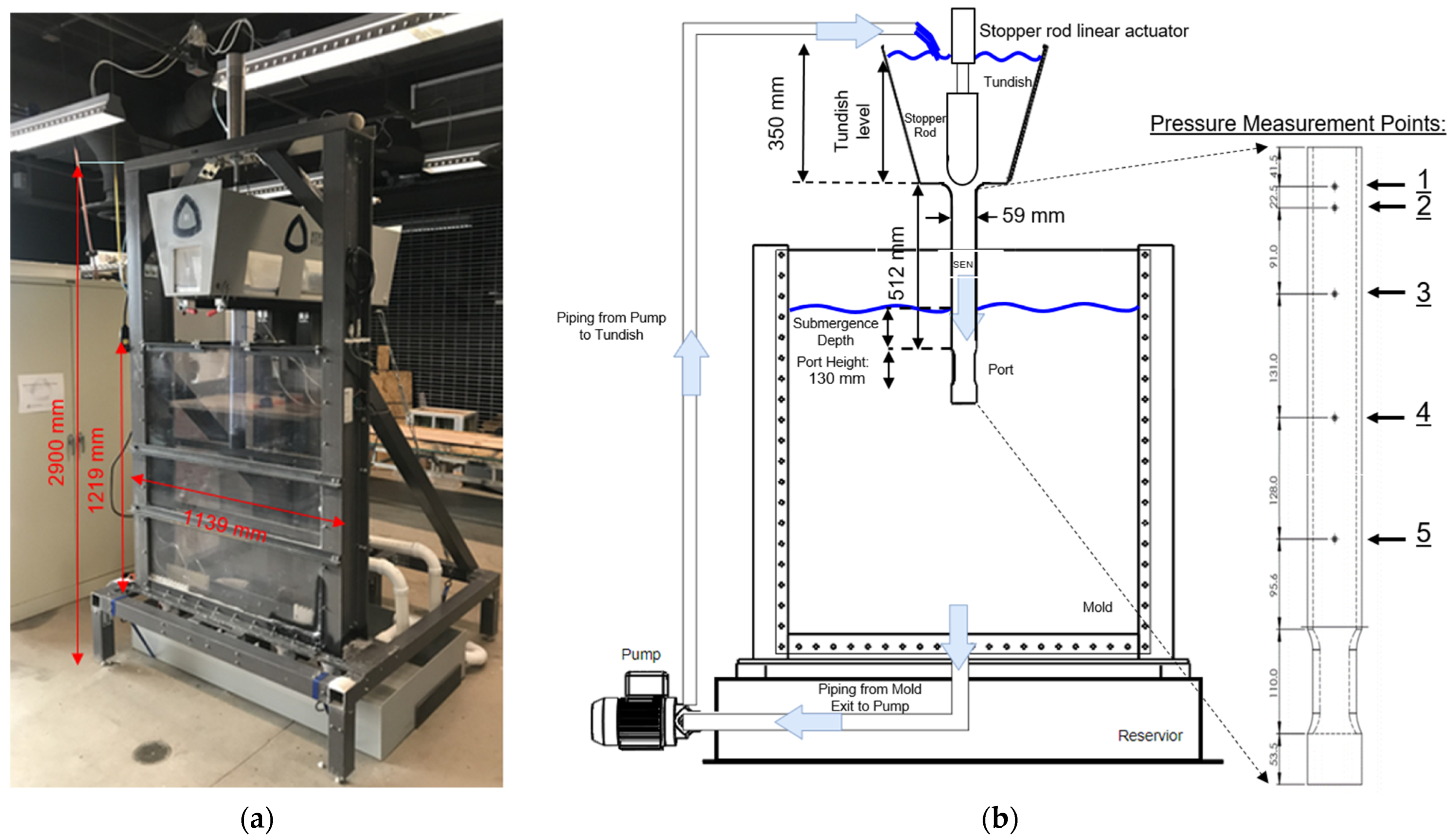
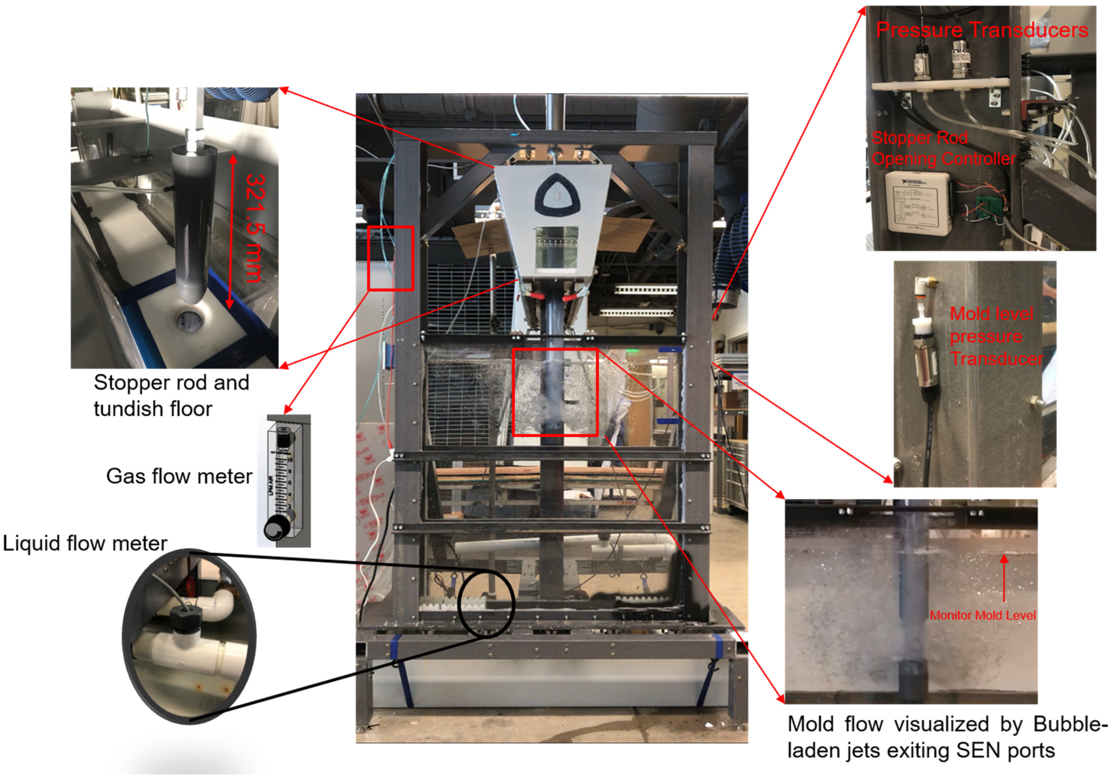
A 0.6-scale water model of a typical continuous caster of steel slabs was constructed at the Colorado School of Mines (Golden, CO, USA) from 2017 through 2020 [71]. As shown in Figure 1 and Figure 2, this physical model is equipped with a tundish, a stopper-rod with a linear actuator and an air injection system, an SEN, mold, a water overflow reservoir, a piping system with a paddlewheel-type water flow meter, and a centrifugal pump, as well as pressure diaphragm transducers to monitor the liquid level in the mold and to measure pressure at different points inside the SEN.

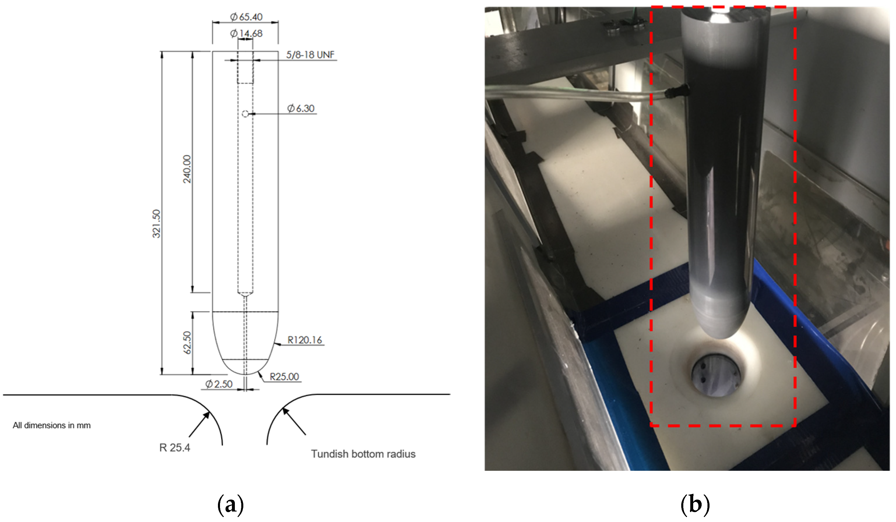
The steel tundish has an epoxy–glass composite floor with a single outlet to deliver water into the SEN. Geometric details of the stopper-rod and the tundish bottom outlet shape are shown in Figure 3. The curved walls of the tundish bottom outlet are typical of an Upper Tundish Nozzle (UTN) in a commercial steel plant. The plastic (poly-vinyl chloride) stopper-rod features a two-radius tip design, which was manufactured via 3-D printing. The stopper contains a drilled central hole for air injection through its tip. The air injection rate into the stopper is measured with a rotameter-type flow meter with max uncertainty +/−0.2 SLPM. Vertical movement of the stopper-rod is achieved by a linear actuator attached to its top with a Teflon (PTFE) coupling. The stopper-rod position is measured with a potentiometer integrated within the linear actuator with an estimated error of +/−1.5 mm. This large uncertainty is due to the flexibility of the plastic tundish bottom floor, which allows some deflection while the stopper-rod closes and then tries to open. Then, during the stopper-rod opening, the unbending of the floor maintains some contact while the stopper-rod moves upward. Therefore, the measurement system shows an opening (up to 1.5 mm) even while there is still no flow through the SEN. Even though efforts were made to compensate for this, some uncertainty remains.

Table 1. Experimental conditions and corresponding real caster conditions.

Casting Conditions	Water Model	Corresponding Real Caster
Tundish Height [mm]	330	550
Casting Speed [m/min]	1.00	1.29
Mold Thickness [mm]	150	250
Mold Width [mm]	1137	1895
Tundish Bottom to Top of Port Distance [mm]	512	852.7
Nozzle Submergence Depth [mm]	55	92
Stopper-Rod Diameter [mm]	65.4	109
Stopper Tip Radius [mm]	25	42
Stopper Bend Radii [mm]	120	200
Stopper-Rod Opening: vertical lift [mm]	14–18	23–30
UTN and SEN Diameter [mm]	59.0	98.3
Absolute Wall Roughness (SEN Walls) [mm]	0.005	0.008
Absolute Wall Roughness (Stopper) [mm]	0.25	0.42
Port Height [mm]	110	183
Port Width [mm]	48.4	81
SEN Wall Thickness [mm]	5	8.3
Tundish Bottom Width [mm]	257	428
Tundish Bottom Length [mm]	1389	2315
Liquid Density [kg/m3]	997	7000
Liquid Flow Rate [tonnes/min]	0.17	4.28
Cold Gas Flow Rate [SLPM]	0–16	0–12
Hot Gas Flow Rate [LPM]	0–16	0–57
Clogging [mm]	0 (everywhere)	0

shows the standard baseline experimental conditions and the corresponding conditions in a full-scale real steel caster. The water model casting conditions and geometry are generally kept constant throughout the parametric studies, except where otherwise indicated for tundish height, submergence depth and gas flow rate. Note that the “corresponding real caster” represents an actual operating commercial caster, except that the dimensions of the nozzle ports in the operating caster are much smaller, and the SEN wall roughness is much larger.

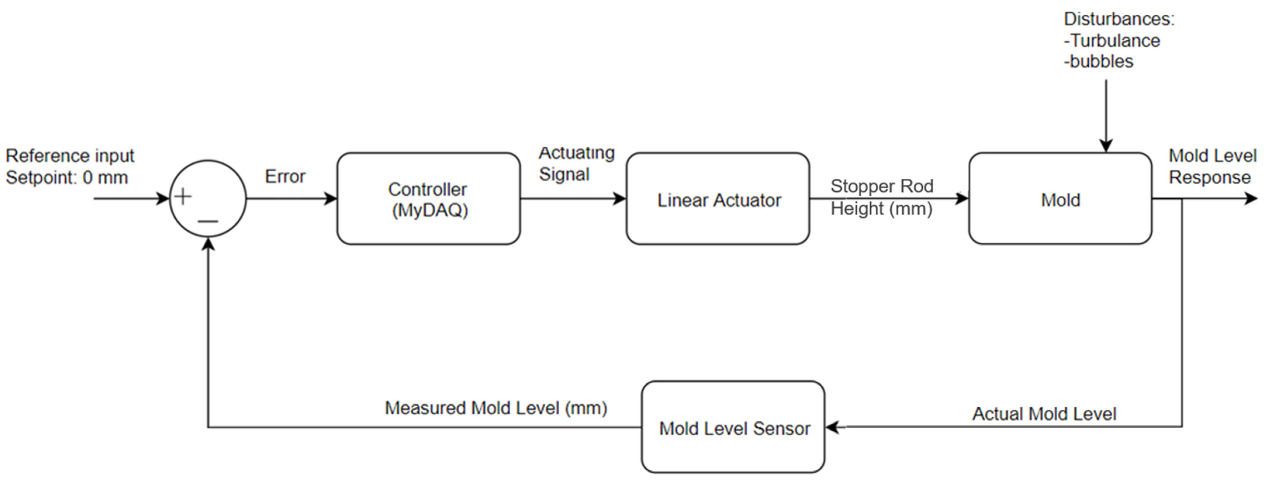
The classic feedback control system of the water model is shown in Figure 4. Its goal was to adjust the linear actuator position to alter the stopper-rod position (vertical opening) and corresponding water flow rate to maintain a constant liquid level in the mold. Error input to the controller is defined by the difference between the user-desired mold level and the height measured by the sensor defines. The linear actuator then adjusts the vertical position of the stopper-rod, which affects the water flow rate into the mold, and, therefore, the level of the liquid surface. This system aims to maintain a steady state mold level to allow the operators to focus on gathering data [71].

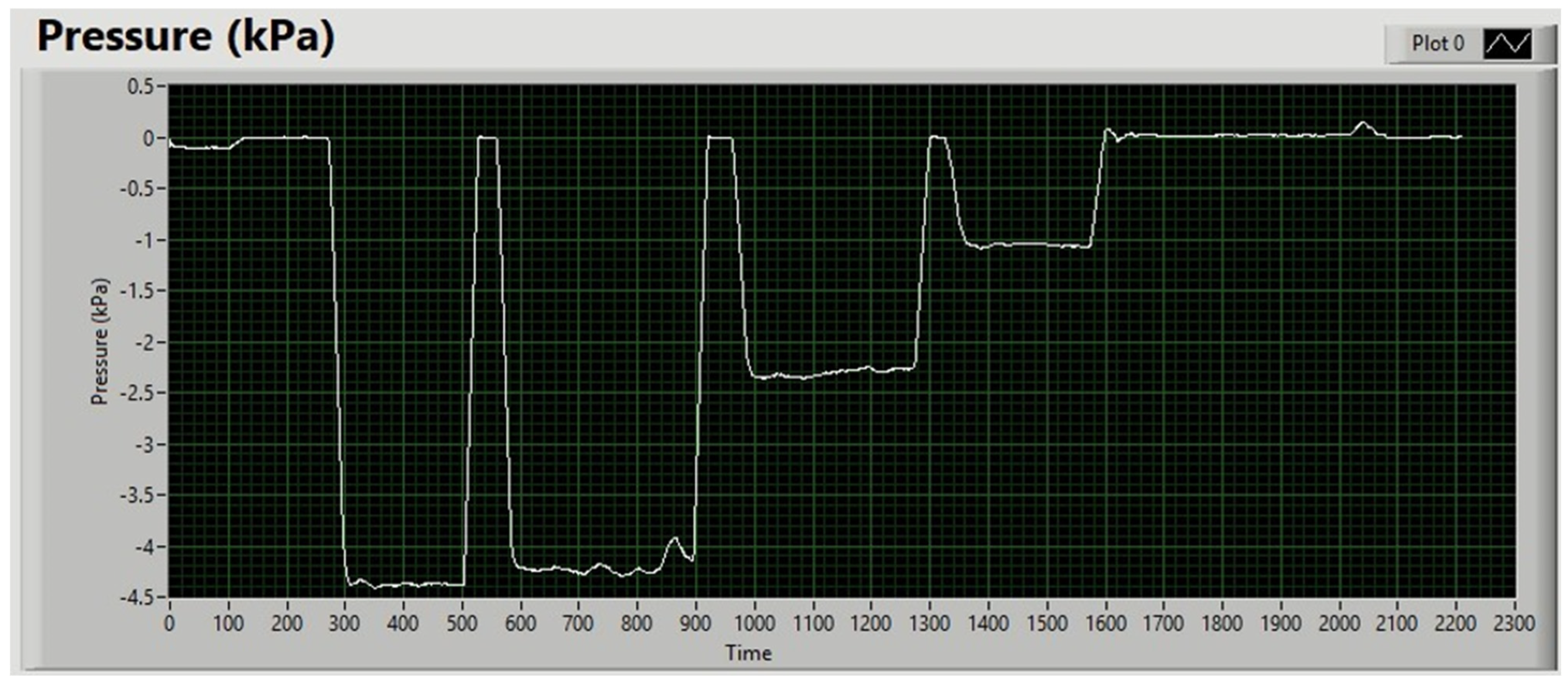
Figure 5 illustrates the CSM water model GUI, showing an example of the recorded pressure for a test with steady-state flow conditions. The tube connected to the pressure sensor is moved between sensing ports during each test to record the pressure at all five locations down the SEN shown in Figure 5. This enables data acquisition at all positions with only one sensor, as shown in Figure 2. The sensor data are collected using a DAQ card that displays the graph and saves it to an Excel file through LabVIEW 2019 [71].

Figure 6 shows the flow stability results of many tests conducted at different stopper-rod openings and air injection rates for other conditions given in Table 1, including constant tundish level and constant pump flow rate for a casting speed of 1 m/min. Results are presented in a grid to map stable operating conditions (cases with green circles and numbers indicating mold liquid level) relative to cases with insufficient flows (red circles) and cases with excessive flows (black triangles). For cases with stopper-rod openings above 20 mm, the liquid level continuously increases, even at smaller air injections, until the water model overflows. This indicates stable casting greater than 1m/min. For cases with stopper-rod openings of 12 mm or less, the liquid level continuously drops until the mold cavity completely drains, regardless of the air injection rate. This indicates that the stable casting speed is less than 1 m/min for these cases. In between, there is an operating window, where the stopper-rod opening can be adjusted (increased between 13 and 18 mm) to compensate for the extra flow resistance caused by the gas injection to enable stable flow without either drainage or overflow.

The contours of the liquid level in Figure 6 show that the stable liquid level increases with increasing stopper opening. This is because increasing the liquid level in the mold decreases the pressure head, which is controlled by the difference between the tundish level and the mold level. This decrease in the gravity driving force can be compensated by increasing the stopper opening. This effect is stronger than the qualitatively similar effect of increasing the gas injection rate, as indicated by the generally shallow average slope of the contour lines. It is interesting to note that increases in air injection rate between 8 and 12 SLPM have a more significant effect on the pressure contour slopes for these conditions, requiring larger stopper opening changes than at other gas flow rates. This suggests important changes in the flow regime for these flow conditions, which will be revealed later.

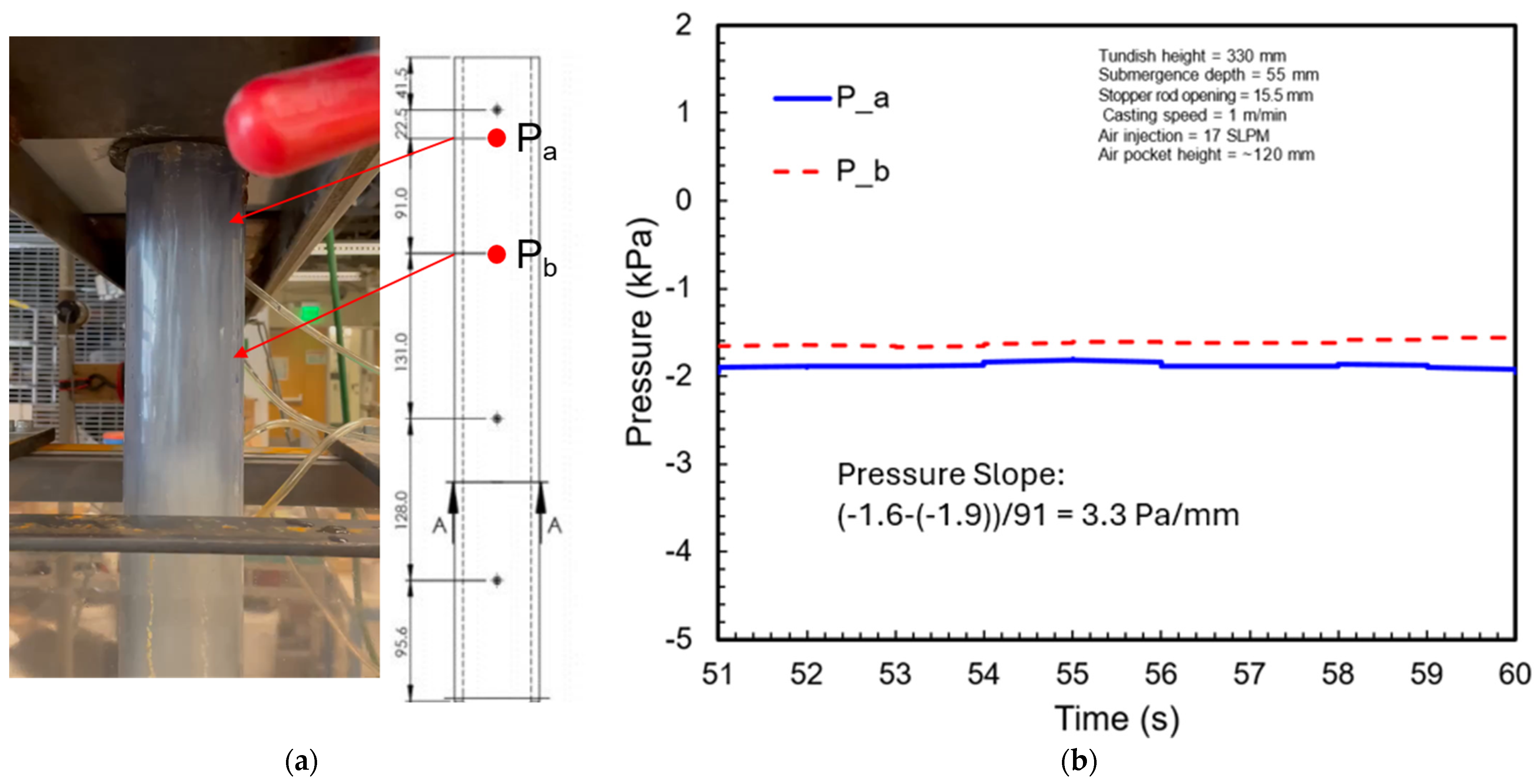
Figure 7 shows pressures measured inside a region below the stopper that contained a large fraction of air. Specifically, the increasing pressure slope from points a to b is ~3.3 Pa/mm. This is much smaller than the hydrostatic pressure increase of ~10 Pa/mm found in the bubbly flow regime of the nozzle. The results here are consistent with previous modeling studies that state that pressure inside an air pocket should be constant [52]. This is because the pressure can equilibrate in a region where the gas phase is continuous. These new results suggest it is rare to obtain a “perfect” gas pocket with fully continuous gas and zero pressure drop. However, these new results confirm the presence of flow regimes with very large gas fractions, which sustain very small pressure drops.

4. New PFSR Model Description

To better understand the results of the water model studies, a computational model was applied to simulate pressure and flow in each experimental case, using a simple but accurate approach validated in previous work [52]. An improved version of the previous PFSR model of pressure and flow rate in stopper-rod continuous-casting systems [52], PFSR V.4.0, is introduced here. Specifically, this version improves PFSR V.3.0 [52] by including a possible gas accumulation region between regions of gas pockets and bubbly flow. PFSR V.4.0 is applied here only to the CSM water model, so, unlike in commercial steel casters, where cavitation was often predicted [52], there is no cavitation for the conditions in this paper.

4.1. Pressure–Energy Model Equations

PFSR solves a one-dimensional system of pressure–energy balance equations (Bernoulli-type), considering kinetic energy, potential energy, and turbulent pressure/energy losses [51,52]. Similar to the approach used for slide-gate systems, PFSG [51], and for stopper-rod systems, PFSR [52], general analytical expressions are obtained for the pressure/energy losses between selected points distributed vertically down the flow system (pictured in Figure 1). Rearranging the pressure drop equations, gauge pressure is calculated at each point by the following:

$$P_i=P_{i+1}+{\rho }_{m}g{h}_{i+1}-{\rho }_{m}g{h}_i+{\displaystyle \frac{1}{2}}{\rho }_m{V_{i+1}}^2-{\displaystyle \frac{1}{2}}{\rho }_m{V_i}^2+{\displaystyle \sum }\Delta P_L$$

(12)

where $P_i$ is gauge pressure of point i [Pa], ${\rho }_m$ is mixture fluid density between points i and i + 1 [kg/m³], $V_i$ is velocity at point i [m/s], and $h_i$ is the height of point i [m]. Details on how the fluid velocities at each point are calculated are discussed elsewhere [51,52]. As the boundary conditions, gauge pressure at the top surface levels of the tundish and the mold are set to 0. Fluid velocities at these two locations, $V_1$ and $V_{10}$, are considered to be negligible [51,52]. The pressure–energy loss terms, $\Delta P_L$ and [Pa], are explained later.

Evaluating Equation (12) for the 12 points in the flow system shown in Figure 8 gives the following 12 equations:

Point 1 (Tundish Level)

$$P_1=P_2-{\rho }_{L}g{h}_{1-2}$$

(13)

Point 2 (Bottom of Tundish)

$$P_2=P_3+{\displaystyle \frac{1}{2}}{\rho }_{L }{V_3}^2+\Delta P_{L,cont}+\Delta P_{L,tun}+\Delta P_{L,two}+\Delta P_{L,stopper}$$

(14)

Point 3 (Minimum Gap)

$$P_3=P_4-{\displaystyle \frac{1}{2}}{\rho }_L{V_3}^2+{\displaystyle \frac{1}{2}}{\rho }_L{V_4}^2+\Delta P_{L,3-4}$$

(15)

Point 4 (Air Pocket Region)

$$P_4=P_{5A}$$

(16)

Point 5A (Bubble Accumulation Zone Entry)

$$P_{5A}=P_{5B}-{\rho }_{mb}g{h}_{5A-5B}-{\displaystyle \frac{1}{2}}{\rho }_L{V_{5A}}^2+{\displaystyle \frac{1}{2}}{\rho }_{mb}{V_{5B}}^2+\Delta P_{L,5\mathrm{A}-5\mathrm{B}}$$

(17)

Point 5B (Inside Bubble Accumulation Zone)

$$P_{5B}=P_{6A}-{\rho }_{mb}g{h}_{5B-6A}-{\displaystyle \frac{1}{2}}{\rho }_{mb}{V_{5B}}^2+{\displaystyle \frac{1}{2}}{\rho }_{mb}{V_{6A}}^2+\Delta P_{Lf,5B-6A}$$

(18)

Point 6A (Bubble Accumulation Zone Exit)

$$P_{6A}=P_{6B}-{\displaystyle \frac{1}{2}}{\rho }_{mb}{V_{6A}}^2+{\displaystyle \frac{1}{2}}{\rho }_{mf}{V_{6B}}^2+\Delta P_{L,6A-6B}$$

(19)

Point 6B (Bubbly Flow Zone Entry)

$$P_{6B}=P_7-{\rho }_{mf}g{h}_{6B-7}-{\displaystyle \frac{1}{2}}{\rho }_{mf}{V_{6B}}^2+{\displaystyle \frac{1}{2}}{\rho }_{mf}{V_7}^2+\Delta P_{Lf,6B-7}$$

(20)

Point 7 (Lower SEN Entry)

$$P_7=P_8-{\rho }_{mf}g{h}_{7-8}-{\displaystyle \frac{1}{2}}{\rho }_{mf}{V_7}^2+{\displaystyle \frac{1}{2}}{\rho }_{mf}{V_8}^2+\Delta P_{Lf,7-8}$$

(21)

Point 8 (Lower SEN Exit, Same Height as Point 9)

$$P_8=P_9-{\displaystyle \frac{1}{2}}{\rho }_{mf}{V_8}^2+{\displaystyle \frac{1}{2}}{\rho }_{mf}{V_9}^2+\Delta P_{L,port}+\Delta P_{L,tee}$$

(22)

Point 9 (Port Exit)

$$P_9={\rho }_{L}g{h}_{sub}$$

(23)

Point 10 (Mold Level)

$$P_{10}=0$$

(24)

where ${\rho }_L$ is the pure fluid density, ${\rho }_{mb}$ is the mixture density in the bubble accumulation zone, and ${\rho }_{mf}$ is the density in the bubbly flow region. These densities are defined as follows:

$${\rho }_{mb}={\rho }_L\left(1-{\alpha }_{mb}\right)$$

(25)

$${\rho }_{mf}={\rho }_L\left(1-{\alpha }_{mf}\right)$$

(26)

where ${\rho }_L$ is the liquid density [kg/m³]; ${\alpha }_{mb}$ is the local gas fraction inside the entire bubble accumulation zone, (5A to 6B), which must be given as input; ${\alpha }_{mf}$ is the local gas fraction in the bubbly flow zone; and $h_{i-i+1}$ is the length (height difference) between points i and i + 1 z. Note that points 6A and 6B are at the same height but are at the boundary between two adjacent zones (bubble accumulation to bubbly flow). Further details on these equations are discussed elsewhere [51,52].

4.2. Velocity and Area Calculations

Velocities are calculated assuming circular cross-sections, as found in the CSM water model. Accounting for the space occupied by the gas, the mixture velocity at each point in the system, $V_i$ is calculated as follows:

$$V_i={\displaystyle \frac{Q_L}{A_{eff,i}}}$$

(27)

where $Q_L$ is liquid flow rate [m³/s], and $A_{eff,i}$ is the effective area of the local cross-section [m²] considering gas injection. Injected gas decreases the effective cross-section area for fluid flow according to its volume fraction, ${\alpha }_i$, which varies with vertical position according to [51,52] as follows:

$${\alpha }_i={\displaystyle \frac{Q_{gas,i}}{Q_{gas,i}+Q_L}}$$

(28)

where $Q_{gas,i}$ is the air flow rate at point i [L /min], which is assumed to model the ‘‘hot’’ argon gas (i.e., at molten steel temperature, $T_{hot}$ = 1823 K) and is calculated in the steel caster from the “cold” gas flow rate at standard conditions as follows [51,52]:

$$Q_{gas,i}=Q_{SLPM}{\displaystyle \frac{P_{atm}}{P_{atm}+\left(\frac{P_i+P_{i+1}}{2}\right)}}{\displaystyle \frac{T_{hot}}{T_{amb}}}$$

(29)

where $Q_{SLPM}$ is the flow rate at standard temperature $T_{amb}=298$ K) injected in standard liters per minute; $P_{atm}$ is the standard (atmospheric) pressure 101 kPa; and $P_{i+1}$ is the gauge pressure at point i + 1 [kPa] (downstream pressure). This equation is inverted to find the cold gas flow rate for the equivalent steel caster in Table 1. In the water model, the hot and cold gas flow rates are naturally the same.

Finally, based on the above equations, the local effective area at point i, $A_{eff,i}$, is calculated [51,52] as follows:

$$A_{eff,i}=A_i\left(1-{\alpha }_i\right)$$

(30)

where $A_i$ is the local cross-section area [m²] of the nozzle at point i, according to the given geometry. The local effective area carries the liquid flow and is used to calculate the local liquid velocity, knowing the total system flow rate and applying a mass balance. In regions of bubbly flow, the liquid and gas velocities are the same and can be used to calculate the gas fraction. In regions of high gas fraction, however, including a gas pocket or the upper length of the new bubble accumulation zone, the effective area is small. Therefore, the liquid velocity is high, and the average gas velocity is lower.

The minimum gap area between the stopper-rod and tundish bottom radius is calculated based on a stopper-rod geometry with three radii: a tip radius and two bend radii [52]. For the CSM water model, the bend radii are equal; hence, the second and third radii have the same value (Table 1).

4.3. Pressure Losses

The extra pressure loss terms in Equations (14)–(22), $\Delta P_{L,cont}$, $\Delta P_{L,tun}$, $\Delta P_{L,two}$, $\Delta P_{L,stopper}$, $\Delta P_{L,port}$, and $\Delta P_{L,tee}$ [Pa] are discussed in detail elsewhere [51,52]. Therefore, only the new and updated terms are presented here. One of the largest pressure drops is between points 3 and 4, which depends on whether the liquid expands or contracts as it flows past the minimum gap, as follows:

$$\{\begin{array}{ll}\Delta P_{L,3-4}={\displaystyle \frac{1}{2}}{\rho }_L{V}_3^2{(1-{\displaystyle \frac{A_3}{A_4}})}^2\hfill & \mathrm{Sudden} \mathrm{Expansion}\hfill \\ \Delta P_{L,3-4}={\displaystyle \frac{1}{2}}\chi {\rho }_L{(V_4)}^2\hfill & \mathrm{Sudden} \mathrm{Contraction}\hfill \end{array}$$

(31)

where $A_3$ and $A_4$ are the cross-section areas of the annular-shaped liquid jet at points 3 and 4, respectively [m²]. $V_4$ is the velocity at point 4 [m/s], which is defined as follows:

$$V_4=\delta V_3$$

(32)

$\delta$ is a fraction between 0 and 1 if the flow expands from point 3 to 4, and it is greater than 1 if the flow is contracting. Expansion is usually expected in both water models and steel casters. Contraction may occur in water models at high air injection rates through the stopper, which pushes the liquid stream to the walls, resulting in high-momentum liquid jets. $\chi$ is the effective fraction of the nozzle diameter with recirculating flow and is defined as follows [52]:

$$\chi ={\left({\displaystyle \frac{1}{\nu }}-1\right)}^2$$

(33)

where $\nu$ is the Weisbach contraction coefficient, as follows [52]:

$$\nu =0.63+0.37{\left({\displaystyle \frac{A_4}{A_3}}\right)}^3$$

(34)

Moving further down the nozzle, $\Delta P_{L,5\mathrm{A}-5\mathrm{B}}$, the expansion pressure drop between points 5A to 5B, caused by the transition from the air pocket region, where liquid jets have high velocity, to the bubble accumulation zone [Pa], where liquid velocity is lower, is defined as follows [51,52]:

$$\Delta P_{L,5A-5B}={\displaystyle \frac{1}{2}}{\rho }_{mb}{V}_{5A}^2{\left(1-{\displaystyle \frac{A_{5A}}{A_{5B}}}\right)}^2$$

(35)

where $A_{5A}$ is the effective cross-section area of the liquid jets at point 5A, just above where the jets impact and $A_{5B}$ is the entire nozzle cross-sectional area at point 5B [m²] inside the new bubble accumulation region; $V_{5A}$ is the velocity of the annular water jet at the bottom of the air pocket region where it hits the bubble accumulation zone. This velocity is constrained as follows [52]:

$$V_{5A}=\sqrt{V_4^2+2g{h}_{air}}$$

(36)

where $h_{air}$ is the air pocket height [m]. Velocity here refers only to the liquid flow and decreases through the upper length of the bubble accumulation zone until reaching point 5B, where liquid velocity stays constant until reaching the end of this zone at point 6A.

Next, a small pressure increase is caused by expansion of the flow at the transition from the high gas-fraction bubble accumulation zone to the lower gas-fraction, higher-density, uniform bubbly-flow region at point 6A to 6B, $\Delta P_{L,6A-6B}$ [Pa]:

$$\Delta P_{L,6A-6B}={\displaystyle \frac{1}{2}}{\rho }_{mb}{V}_{6A}^2{\left(1-{\displaystyle \frac{A_{6A}}{A_{6B}}}\right)}^2$$

(37)

where $A_{6A}$ and $A_{6B}$ are the effective cross-section areas [m²] at point 6A (bottom of the bubble accumulation zone) and point 6B (top of the bubbly flow region), which differ due to the different local gas fractions, even though both regions have primed bubbly flow.

Finally, $\Delta P_{Lf,5B-6A},$ $\Delta P_{Lf,6B-7}$ and $\Delta P_{Lf,7-8}$ are the wall friction losses [Pa] [41,42], as follows:

$$\Delta P_{Lf,5B-6A}={\displaystyle \frac{1}{8}}{\rho }_{mb} f_{SEN}\left[{(V_{5B})}^2{L}_{5B-6A}{\displaystyle \frac{\left(D_{5B}+D_{6A}\right)\left({D_{5B}}^2+{D_{6A}}^2\right)}{{D_{6A}}^4}}\right]$$

(38)

$$\Delta P_{Lf,6B-7}={\displaystyle \frac{1}{8}}{\rho }_{mf} f_{SEN}\left[{(V_{6B})}^2{L}_{6B-7}{\displaystyle \frac{\left(D_{6B}+D_7\right)\left({D_{6B}}^2+{D_7}^2\right)}{{D_7}^4}}\right]$$

(39)

$$\Delta P_{Lf,7-8}={\displaystyle \frac{1}{8}}{\rho }_{mf} f_{SEN}\left[{(V_7)}^2{L}_{7-8}{\displaystyle \frac{\left(D_7+D_8\right)\left({D_7}^2+{D_8}^2\right)}{{D_8}^4}}\right]$$

(40)

where $V_{5B}$, $V_{6B}$ and $V_7$ are velocities at points 5B, 6B and 7 [m/s]; $L_{5B-6A}$, $L_{6B-7}$ and $L_{7-8}$ are lengths of the SEN from points 5B to 6A, 6B to 7, and from points 7 to 8 [m], respectively; $D_{5B}$, $D_{6A}$, $D_{6B}$, $D_7$, and $D_8$ are the nozzle hydraulic diameters at points 5B, 6A, 6B, 7, and 8 [m]; and $f_{SEN}$ is the friction factor in the SEN region, which depends on the relative wall roughness, $ϵ/D_i$, where $ϵ$ is the absolute wall roughness in [m] [47].

4.4. Solution Procedure

Using the input geometry and casting conditions (including the bubble accumulation zone length and gas fraction at the bubble accumulation zone), the fully coupled system of 13 equations is solved simultaneously using the implicit FSOLVE solver in MATLAB v.2022a [72]. These equations are derived from 11 pressure-drop–energy balance equations between the 12 model points and two boundary conditions. These equations are rearranged into 12 equations for the pressures at each point and the error, F₁, from the boundary Equation (13) at the top boundary, which represents the liquid level in the tundish, where gauge pressure should be zero. This approach solves for one missing user-selected unknown (in addition to 12 pressures at 12 points) by minimizing F₁, which minimizes error in the entire system as follows:

$$F_1=P_2-{\rho }_{L}g{h}_{1-2}$$

(41)

The total system of equations has 15 unknowns, consisting of 12 pressures, an air pocket height, expansion/contraction coefficient (δ) at point 4, and any missing casting condition [51,52]. Note that the length of the upper part of the bubble accumulation zone, between 5A and 5B ($h_{5A-5B}$ in Equation (17)), the total bubble accumulation zone length, between 5A and 6B, and gas fraction inside the bubble accumulation zone are required inputs; hence, they are not allowed to be unknown.

With 15 unknowns and only 13 equations, two additional degrees of freedom must be specified to achieve a unique solution. These two can be chosen from any of the following options:

• The missing casting condition (to fully define all casting parameters, such as the stopper-rod opening distance),
• Air pocket height,
• Expansion/Contraction coefficient of flow $\delta$ at point 4, or
• Any gauge pressure within the system, such as pressure at one of points 2, 5–9, might be found from plant measurements or other sources.

The FSOLVE algorithm solves an inverse problem by adjusting the value of the user-selected unknown until the error in Equation (41) is less than the tolerance of 10⁻¹² kJ/m³. This unknown could be almost any model parameter, such as casting condition, velocity, length of a flow region, etc. Convergence is usually very fast, as runs finish in <10 s on a standard personal computer.

5. Results

Parametric studies were conducted with both the experimental water model and the PFSR computational model for base conditions, as shown in Table 1. The only difference is that PFSR simulations assumed the same absolute roughness of 0.005 mm for all surfaces. The following subsections compare measured and predicted results for the flow regime, pressure distribution, and flow velocity for two parametric studies to investigate the effect of varying gas flow rates.

5.1. Flow Regime

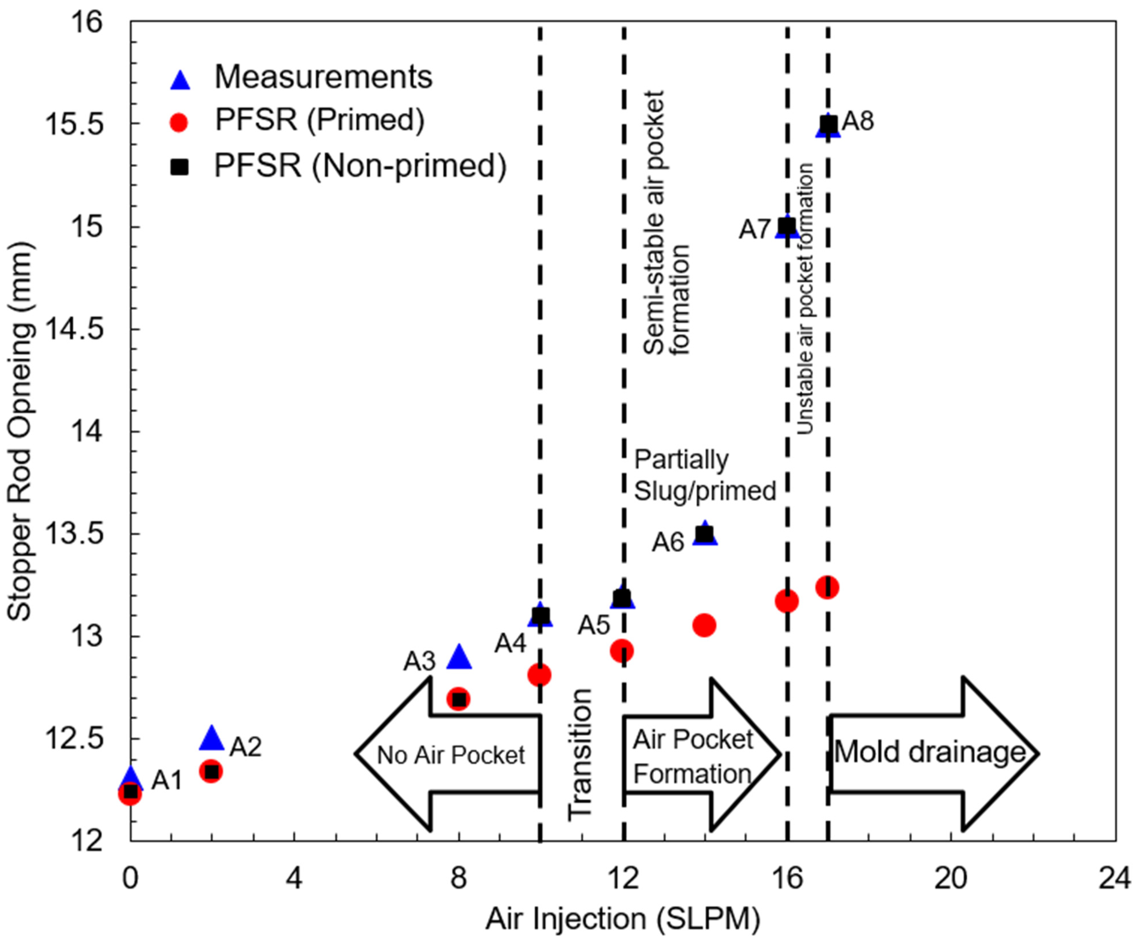
Figure 9 shows experimental measurements taken using the CSM water model, compared with PFSR model predictions, for Cases A1–A8. The casting speed was kept constant at 1 m/min by fixing the pump flow rate. The tundish height and submergence depth were maintained at 330 and 55 mm, respectively, by varying the stopper-rod opening. Other geometrical and casting conditions are given in Table 1. The primed PFSR model refers to PFSR V.2.1 (or PFSR V.3.0 with no cavitation and no air pocket formation) [52], while non-primed PFSR refers to the new model, which includes a bubble accumulation zone.

With less than 10 SLPM air injection, there is no air pocket height formation; hence, the system is fully primed. In this portion of the figure, the flow regime is a fully-primed bubbly flow, and the primed PFSR model matches reasonably well with stopper-rod measurements for all air injection rates. The measurement is always a little higher than the model prediction and grows slightly with increasing air injection, which indicates that there may be a small bubble accumulation region, which was not modelled here.

Increasing air injection from 10 to 12 SLPM, the flow transitions into a regime that is not fully primed but has no significant air pocket. This flow regime has a higher accumulation of gas and bubbles.

Above 12 SLPM air injection, a relatively stable air pocket forms, which partially contains slug flow and evolves into a bubble accumulation region below, followed by a fully-primed flow below that. The deviation in the primed PFSR model prediction increases significantly. The new PFSR model is able to match the measurements exactly.

When air injection exceeds 16 SLPM, unstable air pockets form, with an unstable slug flow regime, and the mold starts to drain. Again, the new non-primed PFSR model was calibrated to match the measured stopper-rod position and the observed air pocket height for each case by adjusting the velocity at point 4. The resulting calculated air pocket heights are shown in

Table 2. Comparison of Measured Air Pocket Height with Non-Primed PFSR Prediction.

Type	Dimension/Condition	A4	A5	A6	A7	A8
Measurements	Gas Flow Rate [SLPM]	10	12	14	16	17
	Stopper-Rod Opening [mm]	13.1	13.2	13.5	15	15.5
	Air Pocket Height [mm]	0–10	0–10	20–30	130–150	200–260
Model Inputs	Expansion Coefficient from Points 3–4, $\delta$ *	0.69	0.70	0.73	0.86	0.84
	Bubble Accumulation Zone Total Length [mm] *	0.	0.	0.	0.	0.
Model Outputs	Air Pocket Height [mm]	3	5	23	140	231
	Stopper-Rod Opening [mm]	13.1	13.2	13.5	15	15.5
	Liquid Velocity at Point 4 [m/s]	3.29	3.3	3.34	3.44	3.29
	$\mathrm{Gas} \mathrm{Fraction}, {\alpha }_{mf}$ in Bubbly Flow Region	0.055	0.066	0.076	0.086	0.091

* indicates calibrated values.

for A-Cases.

Estimation of the corresponding gas flow rates in the steel caster for these flow regimes and transitions is very difficult, as discussed previously. Owing to gas expansion, the critical hot gas flow rate for the transition (16 LPM) is expected to be much higher in the corresponding steel caster (57 LPM) due to the high temperature inside the nozzle. The corresponding critical cold gas flow rate in the steel caster is estimated to be only slightly lower than measured in the water model (~12 SLPM), assuming the same critical gas fraction and that the similarity criteria hold.

5.2. Pressure

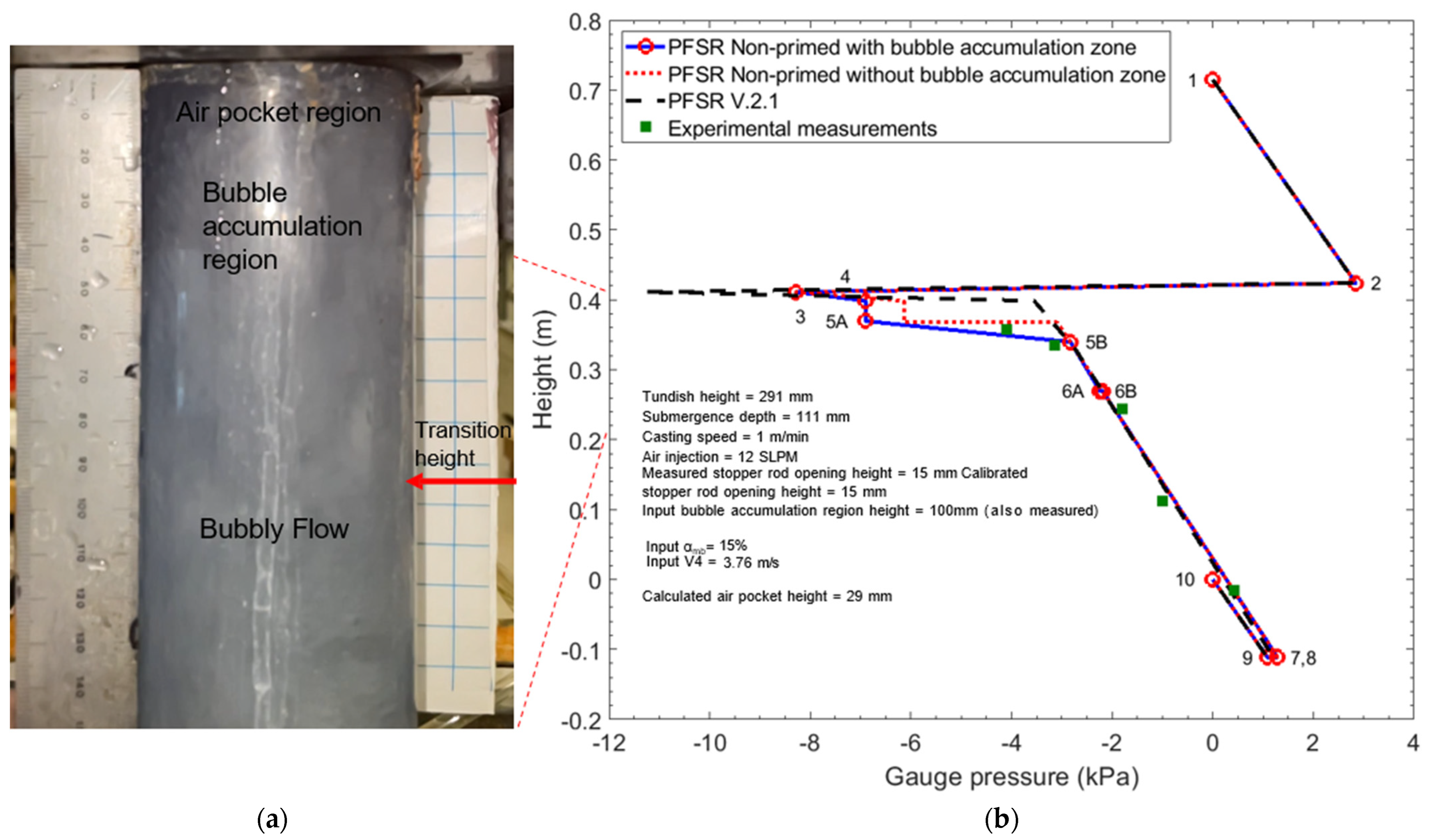
Next, a parametric study of five cases (B-cases) was conducted to compare the new non-primed PFSR model with pressure measurements in the water model. Specifically, pressures were measured (and calculated) at five points, with locations shown in Figure 1b. Except for the changed conditions given in

Table 3. Validation B-cases Conditions.

Type	Dimension/Condition	Cases
		B1	B2	B3	B4	B5
Measurements (and Model Inputs)	Tundish Height [mm]	300	280	291	307	320
	Gas Flow Rate [SLPM]	0	3	12	12.5	13
	Submergence Depth [mm]	95	152	111	87	135
Measurements (Additional)	Air Pocket Height [mm]	0	0	20–30	30–40	30–40
	Stopper-Rod Opening [mm]	14	15	15	15	15
Model Inputs: Calibrated for PFSR (Non-Primed)	Stopper-Rod Opening [mm]	14	15	15	15	15
	Expansion Coefficient from Points 3 4, $\delta$	0.79	0.83	0.92	0.95	0.95
	Bubble Acc. Zone Upper Length 5A–5B [mm]	0.07	80	30	50	40
	Bubble Acc. Zone Total Length 5A–6B [mm]	0.1	100	100	100	100
	$\mathrm{Gas} \mathrm{Fraction} \mathrm{in} \mathrm{Bubble} \mathrm{Acc}. \mathrm{Zone}, {\alpha }_{mb}$	0	0.02	0.15	0.13	0.19
Model Outputs PFSR (Primed)	Stopper-rod Opening [mm]	13	13.8	14	13.6	14
	Velocity in Bubbly Flow Region	1.04	1.06	1.11	1.12	1.12
	$\mathrm{Gas} \mathrm{Fraction}, {\alpha }_{mf}$ in Bubbly Flow Region	0	0.017	0.066	0.068	0.071
Model Outputs PFSR (Non-Primed)	Air Pocket Height [mm]	0.1	0.2	29	38	32
	Liquid Velocity at Point 4 [m/s]	3.49	3.37	3.76	3.86	3.88
	Velocity in Bubbly Flow Region	1.04	1.06	1.11	1.12	1.12
	$\mathrm{Gas} \mathrm{Fraction}, {\alpha }_{mf}$ in Bubbly Flow Region	0	0.017	0.066	0.068	0.071

, all other input conditions are the same as in Table 3.

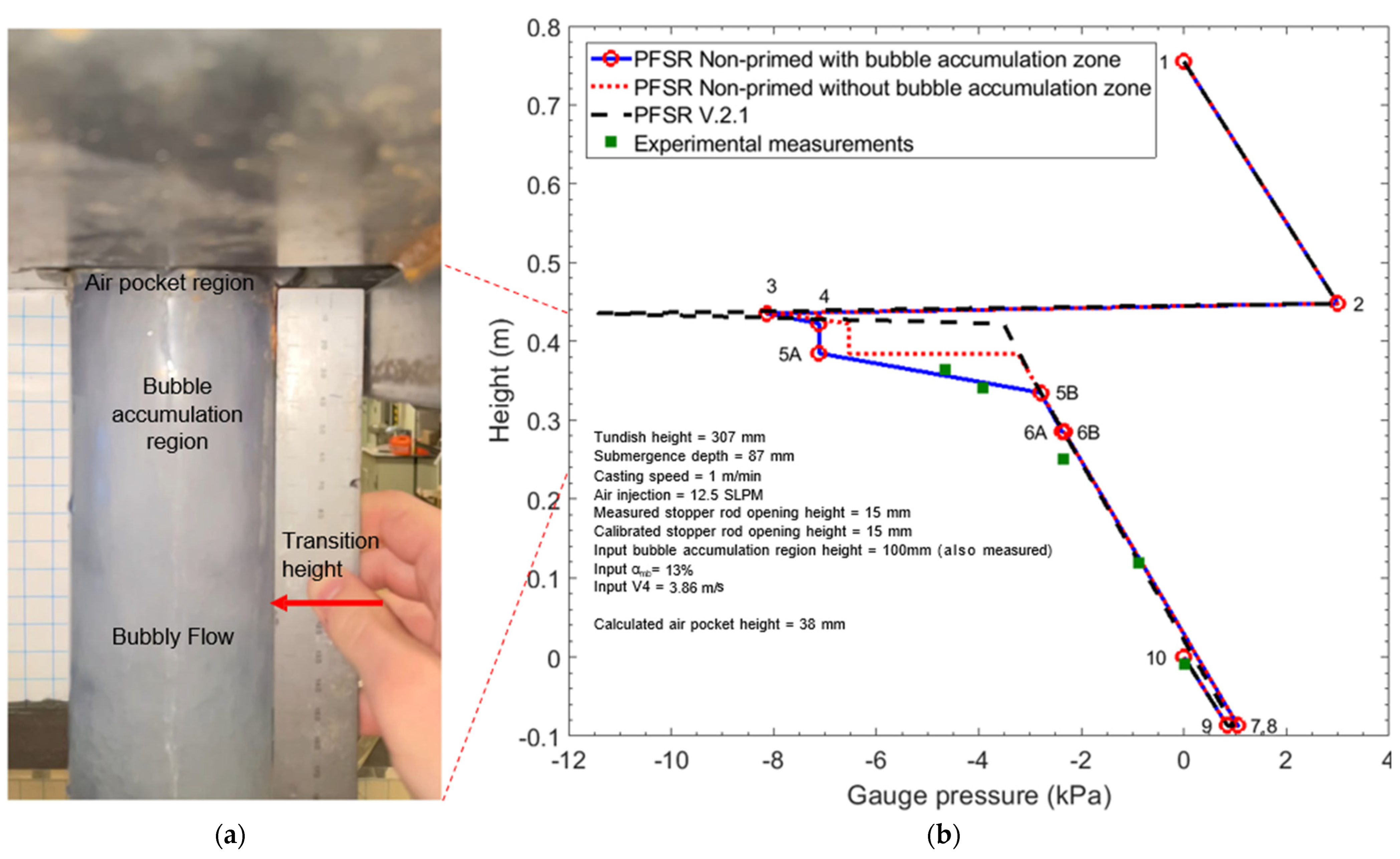
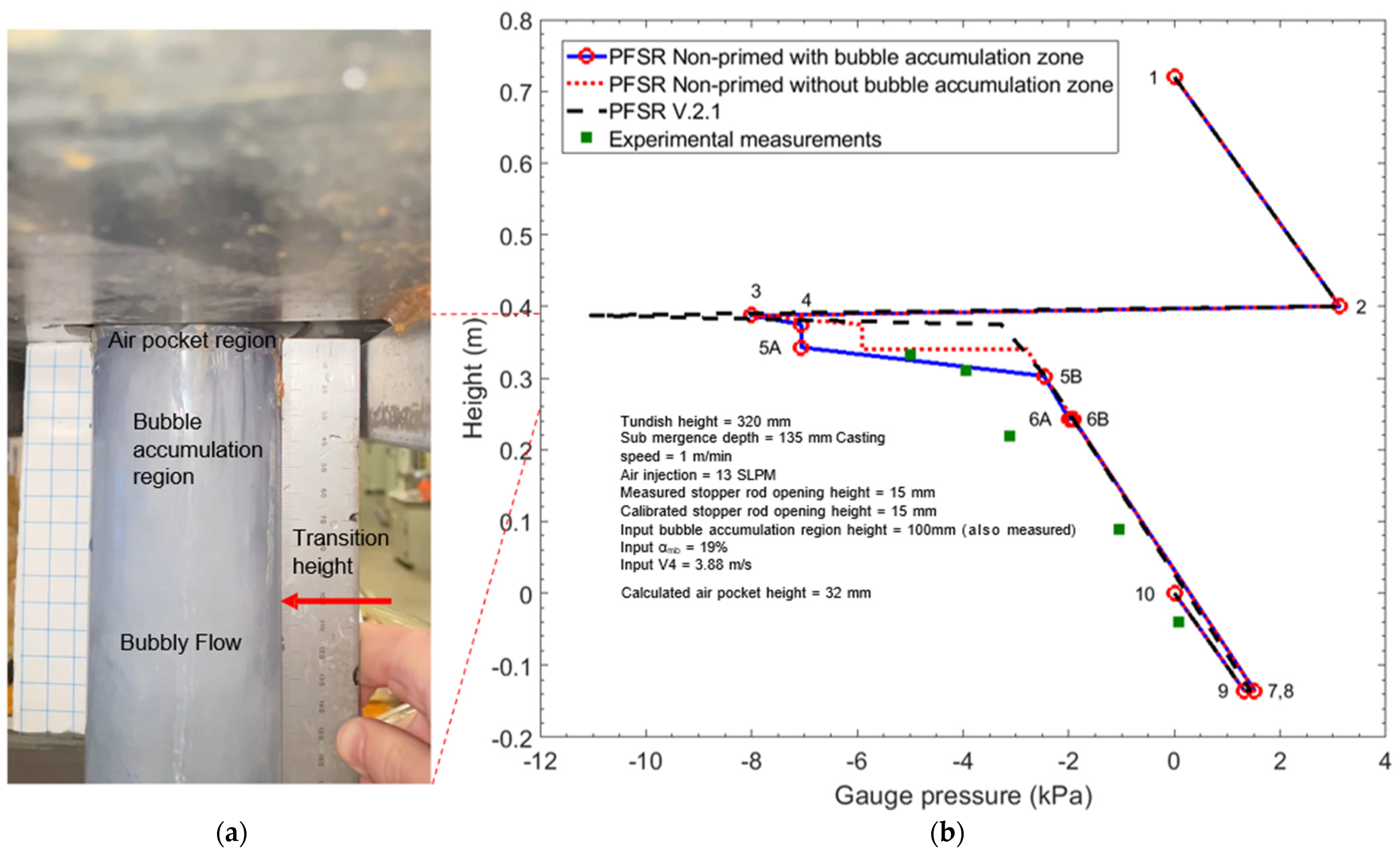
Figure 10, Figure 11, Figure 12, Figure 13 and Figure 14 compare the pressure distributions predicted by the primed and non-primed PFSR models, along with the measurements for Cases B1–B5. For cases B1 and B2, the flow is fully primed. The pressure distributions calculated by the primed PFSR model almost match the pressure measurements, except at measurement points 1 and 2, just below the stopper tip. This mismatch is likely due to the highly turbulent recirculating flow just below the stopper tip, which is difficult to capture with a 1-D model [52]. The PFSR non-primed model with a bubble accumulation zone, however, matches the measurements much better, especially for case B2 (3 SLPM air injection).

Note that the pressure distributions of the two models do not exactly match, even for these two primed flow cases (no air pocket). This is because the stopper-rod openings are slightly different.

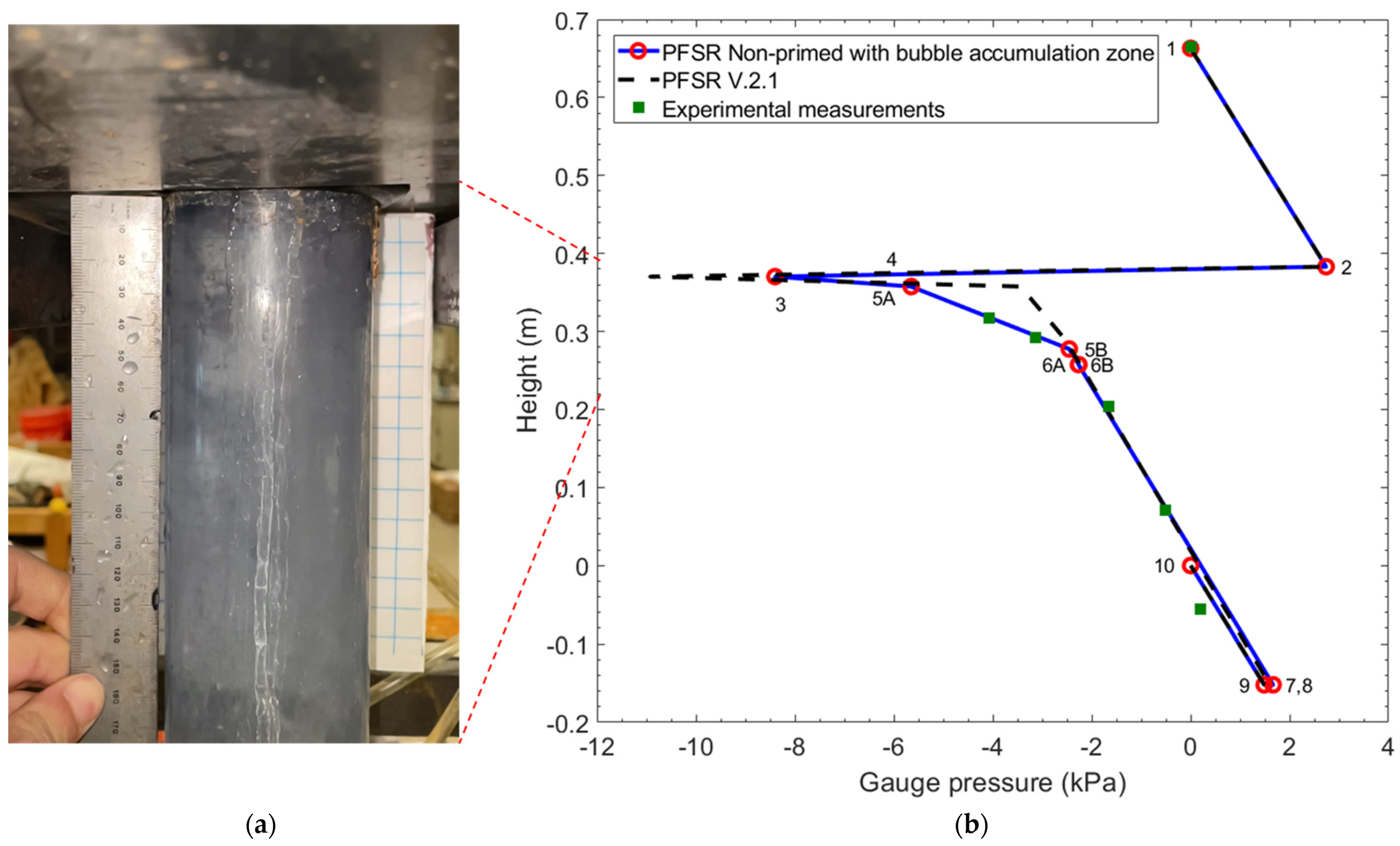
As gas injection increases, gas pockets and bubble accumulation regions increase in likelihood and size. Therefore, the non-primed PFSR model was applied to improve upon the prediction of case B3. This was accomplished by inputting two lengths, a gas fraction for the bubble accumulation zone and an expansion fraction $\delta$, (which defines the velocity at point 4) while outputting the gas pocket length and various velocities, as given in Table 3. As shown in Figure 10, the new model pressure prediction matches even better with the pressure measurements, specifically at the high-gas-fraction points 1 and 2 (5A and 5B).

Note that the new bubble accumulation zone, between points 5A and 5B, shows a large increase in pressure, with a large slope (~140 Pa/mm), relative to elsewhere in the nozzle. This is due to the liquid flow expanding and experiencing a large increase in cross-sectional area from where the annular liquid jets impact the bottom of the air pocket region at point 5A to within the bubble accumulation zone at point 5B, which has an effective area of almost the entire nozzle cross-section. This causes the liquid velocity to decrease significantly from points 5A to 5B. The associated loss of kinetic energy is transformed into a large pressure increase, which is seen in both the measurements and PFSR calculations in this region.

In the lower portion of the bubble accumulation zone (points 5B to 6A), the pressure slope drops to only slightly higher than in the bubbly flow region, but the difference is difficult to discern in the figure. Finally, the bubbly flow region, where the velocity is lowest, has an even smaller pressure slope (~10 Pa/mm).

The new non-primed PFSR model was next applied to cases B4 and B5, which also have high gas injection rates. The same method was used for cases B3–B5, and Table 3 gives the input and output data. The same improvement in agreement with the pressure measurements was found, as illustrated in Figure 13 and Figure 14. It is important to note that for each of these three cases, the calculated air pocket height is in the range of the measurement observations.

5.3. Velocity

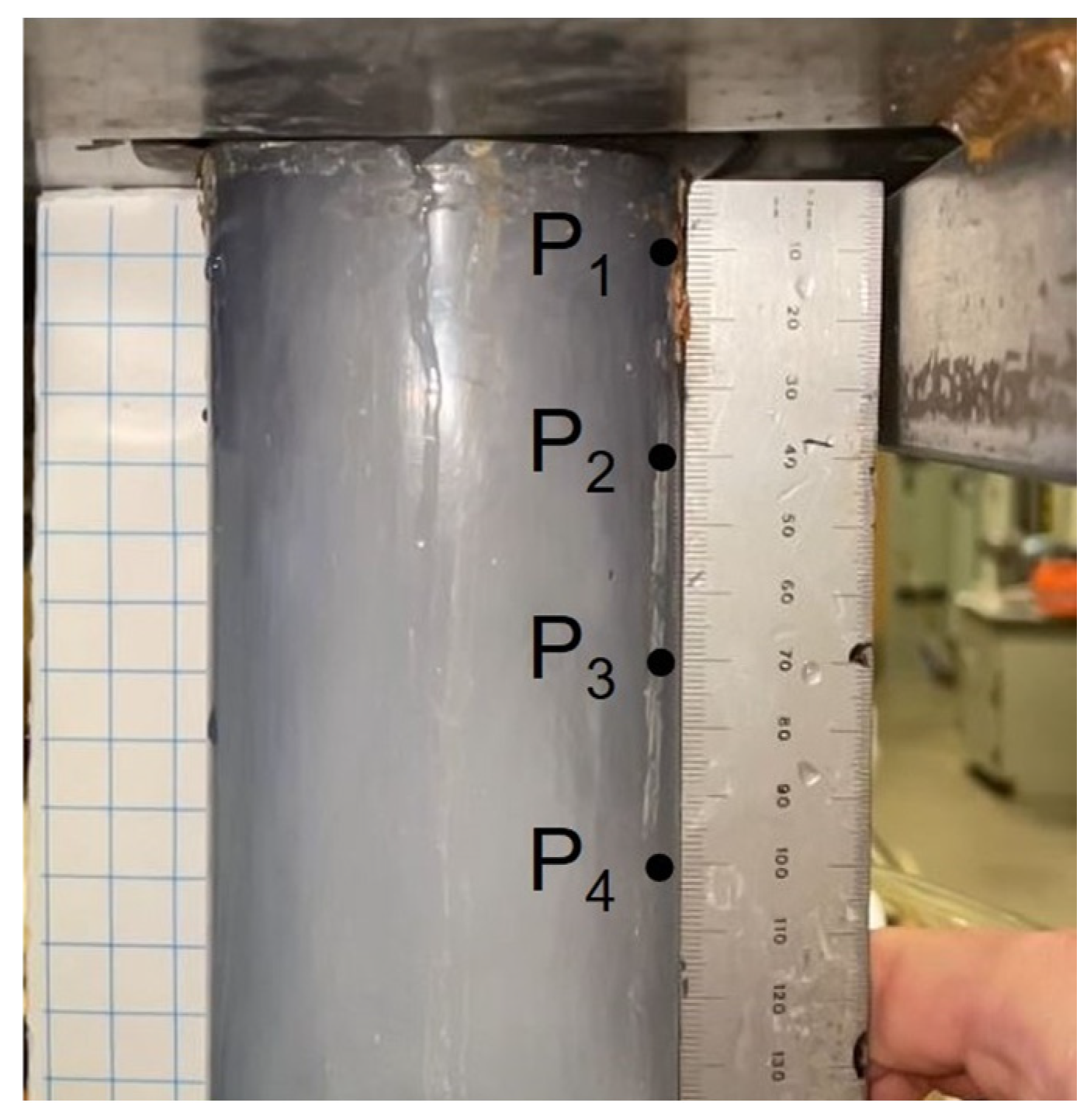
Next, velocity measurements were conducted for both the primed and non-primed B cases to compare with the model predictions. For each case, videos were recorded on an iPhone 14 Pro Max (Apple, Cupertino, CA, USA) camera at 240 frames per second (FPS) for about 2 min. Next, VLC Player v3.0.18 x64 with millisecond precision was applied to playback videos at 30 FPS. For each case, velocity was estimated from the video images at four points down the nozzle, P₁ to P₄, which have 30 mm spacing. Their relative distances from the top of the plate are d1 = 10 mm, d2 = 40 mm, d3 = 70 mm, and d4 = 100 mm, as shown in Figure 15. Knowing the travelled distance and the elapsed time between video frames, the instantaneous velocity is estimated as follows:

$$V={\displaystyle \frac{\Delta x}{\Delta t}}$$

(42)

The distance travelled by random particles in the flow (typically small gas bubbles) over the roughly 30 mm distance (from about 15 mm above the point to about 15 mm below the point) was measured from the photographs over the fixed time interval of 33 ms between adjacent frames in the video playback. This gives average velocity at four points along a 120 mm vertical region near the top of the nozzle (see Figure 15). To improve accuracy, this velocity calculation procedure was repeated for each case by measuring four different particles, taken at time intervals of about 20 s. The average of each of the four measured velocities is presented in

Table 4. Flow velocity in the nozzle at different points for B cases.

Location	Case B1		Case B2		Case B3		Case B4		Case B5
	Meas.	PFSR	Meas.	PFSR	Meas.	PFSR	Meas.	PFSR	Meas.	PFSR
P1 (@ 5A)	1.00	1.04	1.03	1.06	3.85	3.84	3.92	3.96	4.00	3.96
P2	1.00	1.04	1.03	1.06	2.07	-	2.11	-	2.15	-
P3 (@ 5B)	0.99	1.04	1.03	1.06	1.16	1.22	1.18	1.20	1.28	1.28
P4 (@ 6B)	0.99	1.04	1.03	1.06	1.04	1.11	1.06	1.12	1.12	1.12

for each case, together with the corresponding predictions from the non-primed PFSR model.

It is important to note that P₁, P₃, and P₄ refer to the velocity measurement locations (Figure 15), and their corresponding locations in PFSR are 5A, 5B, and 6B, respectively (Figure 8). However, point P2 is inside the bubble accumulation zone between points 5B and 6A; hence, it is not included directly in the PFSR.

For cases B1 and B2, the velocity is almost constant in this upper region of the nozzle because the flow is fully primed. Its value matches a classic mixture velocity calculation for bubbly flow, as also found in the lower nozzle. For cases B3, B4, and B5, however, liquid velocity is much higher towards the top of the nozzle, where the flow is non-primed and contains large gas fractions. Once the annular liquid jets from the stopper merge together to ensure that the flow extends across the entire cross-section of the nozzle, the liquid flow velocity becomes lower and relatively uniform. This is found in both the measurements and the model predictions, which match well with the measurements.

In all non-primed flow cases, the liquid velocity is highest at the bottom of an air pocket below the stopper, where the annular liquid jets from the stopper gap contract in a cross-sectional area and accelerate as in a waterfall. Upon hitting the gas accumulation zone, these jets rapidly decelerate (from points 5A to 5B), as mentioned earlier. The decrease in liquid velocities through this region is quantified by both the measurements and calculations in Table 4. These liquid velocities in Table 4 are greater than the corresponding average gas velocities, owing to the high gas fraction in this zone. In the lower portion of the bubble accumulation zone (points 5B to 6), the liquid velocity is constant and lower. The average gas velocity is even lower. Finally, in the bubbly flow region that comprises most of the lower nozzle, the flow is uniform as liquid velocity decreases even further and gas velocity increases to reach the same constant value.

6. Conclusions

This work presents a new 0.6-scale experimental water model, as well as a new MATLAB-based program to study non-primed multiphase flow in water models of steel continuous casting with gas injection. The new water model at Colorado School of Mines includes the tundish, stopper-rod, submerged entry nozzle and mold region of a continuous slab caster. It includes an air injection system, a pumping system for water recirculation, and a control system to regulate stopper-rod movement to maintain a stable liquid level. It also features measurements of air and water flow rates, mold level, stopper position, pressure at multiple locations, and some velocities.

The new computational model, PFSR V4, solves a one-dimensional system of Bernoulli equations for the pressure distribution and flow rate in stopper-rod nozzle systems for air–water flow systems. This model improves existing models [52] by allowing a new bubble accumulation zone between the air pocket and bubbly-flow regions. This new region can improve the pressure prediction to match better with water-model measurements [52].

Parametric studies with the water model showed that the flow regime is fully primed bubbly flow at low gas flow rates. Increasing the gas flow rate above 10–15 SLPM in the water model (estimated to be slightly less in the corresponding real steel caster) causes a gradual transition to non-primed flow with three different flow regimes inside the nozzle. These consist of a possible air pocket region just below the stopper-rod, a transition region where gas bubbles accumulate to produce a high gas fraction, and a large region of classic, bubbly flow in the lower SEN, where the gas fraction is low. When gas flow exceeds a critical rate, the bubble accumulation region grows rapidly, the flow becomes unstable, and the mold level becomes difficult to maintain with the current system. Although the hot gas flow rates needed for these transitions are expected to be much higher in the real caster, owing to the gas expansion at liquid steel temperature and lower pressure, the critical cold gas flow rate is estimated to be only slightly lower.

The measurements also confirmed the model assumption that pressure change within an air pocket region is relatively small. Pressure below the stopper then increases greatly as the annular liquid jets decelerate through the upper portion of the bubble accumulation zone. Furthermore, both the measurements and model calculations show that the downward liquid flow velocity in this high-gas-fraction region of gas bubble accumulation is much faster than the classic mixture velocity observed in the bubbly-flow region below. In the fully-primed, uniform-velocity, bubbly-flow region that comprises most of the nozzle, the pressure increase is intermediate and is readily predicted with the multiphase model.

Finally, the new PFSR V.4.0 model can be calibrated to match the different flow regimes observed in the water model. The model then shows a very reasonable match with the water-model measurements of both pressure and velocity, with a maximum error in velocity of 7%. The new PFSR model is ready to be applied in future work to investigate pressure drops and flow rates in real continuous casting systems with stopper-rod flow-control systems.

7. Future Work

There are many ways to improve our new PFSR model in future work. A comparison with advanced CFD of the multiphase flow could reveal additional insights to provide more equations and constraints on the PFSR model’s degrees of freedom in order to make it a more predictive model. The CFD model should include gas pockets, bubble size distribution evolution, bubble coalescence and breakup, pressure and temperature-dependent gas expansion, and other important phenomena. Better water model measurements could apply advanced sensors, such as Particle Image Velocimetry (PIV) and high-speed cameras, to accurately measure gas fractions and velocity profiles to validate the model improvements.

Finally, PFSR should be applied to real continuous steel casting conditions, including the effects of temperature and pressure on gas expansion. The predictions should be compared with pressure measurements in the real plant. A better understanding would enable better equations for scale-up and interpretation of water model measurements. An accurate PFSR model of the steel caster could be applied in parametric studies to investigate improved stopper and nozzle designs, gas injection locations, and bore shapes prior to expensive plant trials and implementation.