Abstract
High-performance control valves are essential components in power plants. High-parameter control valves are specialized valves for controlling high-pressure, high-flow, high-temperature, and highly corrosive media. Control valve performance is critical for the stable operation of power plants. The multi-stage counter-flow passage is a common structure in pressure-reducing control valves, effectively mitigating cavitation and erosion on the valve walls. However, in practice, vibration issues in multi-stage passage valves are particularly pronounced. This study employs FSI (fluid–structure interaction) to simulate the vibration characteristics of multi-stage passages. Flow field data for the multi-stage passage are obtained through FLUENT software. A time-frequency analysis of the lift coefficient in the multi-stage passage flow field was performed. The vibration characteristics of the valve core’s inlet and outlet surfaces were studied using Transient Structural software. The results show that when high-pressure fluid passes through the valve core’s passage, it undergoes buffering, steering, and rotating motions, leading to a gradual pressure drop and generating resistance and lift. These phenomena are primarily caused by vortex shedding in the flow field, with the dominant frequency observed to be approximately 5400 Hz. Additionally, as the valve core progresses through the P1 phase at the inlet and the P2 phase at the outlet, the vibration intensity gradually decreases, reaching a minimum in the sixth phase, before increasing and peaking in the final stage. Analysis of the flow field characteristics within the valve core passage reveals the significant impact of vortex shedding on the valve core’s vibration and lift. Phase analysis of the valve core’s vibration intensity further clarifies its behavioral changes at different operational stages. These findings help optimize the design of multi-stage buffering valve cores, improving their performance and stability.
1. Introduction
High-parameter control valves are essential components in power plants. These valves control high-pressure, high-flow, high-temperature, and highly corrosive media. Severe cavitation, erosion, and flow instabilities induced by turbulence can occur inside the valves during the construction and operation of supercritical units. Fluid–solid interaction can cause severe vibrations in the valves and connected pipelines, potentially leading to system destruction and significant economic losses. Vibrating valve components and pipelines can deform internal parts or the pipelines, affecting flow field distribution and causing significant deviations from design values, threatening control system stability. The multi-stage counter-flow passage is commonly used in pressure-reducing control valves to effectively mitigate cavitation and erosion on the valve walls. Despite recent advancements, several critical limitations persist in current research. For instance, the vibration mechanism of multi-stage flow channels lacks in-depth analysis, and the accuracy and reliability of numerical simulations require further improvement. Additionally, experimental data must be more comprehensive and precise to ensure robust validation. Therefore, a systematic investigation into the vibration mechanisms and dynamic characteristics of multi-stage flow channel valves is imperative. With the rapid development of computational fluid dynamics (CFD), numerical simulation has become an indispensable tool for analyzing valve flow fields and vibration behavior. CFD enables the direct visualization of internal flow patterns and facilitates the assessment of flow-induced vibrations, thereby providing a theoretical basis for valve optimization and performance enhancement. However, numerical simulations alone are insufficient; experimental validation remains essential to verify their accuracy. By correlating simulation results with experimental data, the reliability of numerical models can be significantly improved. Integrating high-fidelity simulations with rigorous experimental testing will enable a more comprehensive understanding of the vibration mechanisms in multi-stage flow channel valves. Such a combined approach will yield a robust theoretical foundation for practical valve design and application.
Fluid-induced vibration can be categorized into two types: longitudinal and transverse, distinguished by the direction of the movement. Longitudinal vibrations occur parallel to the axis, whereas transverse vibrations happen at a perpendicular angle to it. Even with minimal flow rates, transverse flow can induce tube vibration. Various flow velocities result in distinct vibration phenomena, such as vortex-induced vibration, turbulent buffeting, fluid elastic instability, and acoustic resonance. Since the 1970s, substantial advancements have been achieved in the comprehension of fluid-induced vibrations in tube bundle structures. The control valve plays a pivotal role, significantly influencing the safe and cost-effective functioning of a nuclear power plant’s pipeline system. Lin et al. [1] conducted a study on the vibration characteristics of a sleeve control valve, clarifying the origins of the vibrations that arise from the flow rates within the valve. Jiang et al. [2] undertook an analysis on the vibration fatigue life of liquid-filled pipelines under external random excitation and internal flow-induced vibrations, employing both finite element simulation and practical experiments. Their research provides valuable guidelines for evaluating the vibration fatigue life and for the anti-fatigue design of liquid-filled pipelines. Zachwieja et al. [3] utilized known vibration velocity, amplitude, and frequency as kinematic inputs to ascertain the maximum strain, thereby determining the stress–strain state of the pipeline and subsequently addressing the failure issues in engineering pipelines. Yang et al. [4] addressed the significant vibration issue in the outbound process pipeline at a natural gas transfer station by proposing a structural innovation methodology. This approach was designed to eliminate vibrations in non-compressor pipelines through a combination of experimental research and numerical simulations. The team carried out vibration tests and spectral characteristic analyses across diverse operational conditions, successfully pinpointing the main sources of pipeline vibration. As a result, they proposed effective strategies to reduce pipeline vibrations. Bolin et al. [5] clarified the mechanism responsible for the vibrations caused by the unsteady flow around the valve core, and performed an analysis on the valve core’s unsteady flow, noise, and vibration characteristics. Within the oil transmission station, the plunger action of the positive displacement pump produces a significant amount of vibrational effects. Lu et al. [6] illustrated that by optimizing the resonance between the pipeline and equipment, the support for the pipeline can be alleviated, and its natural frequency can be increased to reduce the impact of pipeline vibrations. This study provides significant insights for the engineering design of positive displacement pump pipeline systems. Presently, there is a dearth of research that concentrates on the coupled interaction between fluid and structure. Zhang et al. [7] undertook a study to investigate the vibration characteristics of axial flow pumps, employing a bidirectional iterative fluid–structure coupling method. Their findings revealed the time-frequency patterns of fluid pressure pulsation and structural vibration at corresponding locations within the axial flow pump. Pei et al. [8] conducted a study on the deformation and stress within the impeller, providing reliability and specific theoretical guidance to ensure the optimal design of pump device structures. Nevertheless, international standards do not adequately address the acceptance and screening criteria for pipeline vibration in relation to structural integrity. Oinonen [9] conducted a study on this subject, and the results suggested that the inherent vibrations of pipeline structures could be activated by high-intensity non-harmonic forces. Wang et al. [10] undertook a thorough investigation into the pressure pulsation characteristics of hose pumps throughout the entire flow channel under diverse operating conditions, employing both numerical simulation and experimental approaches. Their objective was to improve the operational reliability of the pump during the optimization phase of pump design. Chen et al. [11] expanded upon this by utilizing a bidirectional fluid–structure coupling method to examine the vibrational behavior of fluids on both the shell side and tube side, in relation to the elastic tube bundle, under varying inlet velocities. Wang et al. [12] subsequently employed the bidirectional coupling fluid–structure interaction (FSI) method to analyze the corresponding structural vibration characteristics, providing a significant reference for the design of tubular pumps. Chen et al. [13] validated the effectiveness of their proposed semi-analytical model by comparing the natural frequencies and mode shapes of valves and pipes derived from ANSYS 2020 R2 finite element simulations and experimental data. The results demonstrated that the errors in natural frequencies for each order were less than 5%, offering valuable insights for the investigation of natural frequencies and mode shapes in flow channels. Jin et al. [14] explored the pressure reduction mechanism within the flow channel of a pressure-reducing valve, establishing a theoretical foundation for the study of flow channel vibration protection discussed in this paper. As a critical component in fluid control systems, the pressure reduction mechanism in the flow channel not only influences valve performance but is also intrinsically linked to the dynamic behavior of the fluid. Liu et al. [15] developed a three-dimensional model of the flow and solid fields in a gas proportional valve using a bidirectional fluid–structure interaction (FSI) coupling method. This study analyzed flow field characteristics and valve core stability, providing significant guidance for safety predictions related to valve core behavior. Sun et al. [16] examined the time and frequency domain results of stem-end vibrations in a control valve under supercritical flow conditions at varying degrees of openness. Xie et al. [17] investigated the impact of fluid–structure interaction on the calculation of modal frequencies for large pneumatic valve plugs, highlighting its non-negligible influence on the dynamic response of pressure pipeline safety valve systems. To further explore this mechanism, Zong et al. [18] designed a test platform incorporating vessels, pipes, and valves, enabling an in-depth analysis of their combined working behavior. Ren et al. [19] confirmed the accuracy of computational fluid dynamics (CFD) methods through experimental validation. Ye et al. [20] introduced a fluid–structure coupling analysis method based on the scaled boundary finite element method (SBFEM). By employing SBFEM to construct semi-analytical models for both the structural and fluid domains, the study investigated the fluid–structure coupling characteristics of liquid oscillation. This approach provides a novel perspective for understanding complex fluid–structure interactions, particularly at the intersection of fluid dynamics and structural mechanics.
Although the vibration mechanisms induced by complex valve flows have been extensively studied in recent years, research on the fluid–structure interaction (FSI) in multi-stage hedging channels remains limited. Current literature predominantly focuses on single flow channels or simplified models, which fail to capture the intricate multi-scale and multi-physics phenomena inherent in multi-stage hedging systems. The present study addresses this critical gap by employing high-fidelity FSI simulations to elucidate the vibration response mechanisms of multi-stage hedging channels under fluid excitation. To further advance understanding, this work introduces an advanced time-frequency analysis methodology to characterize the transient lift coefficient of the flow field, enabling the precise identification of instantaneous dynamic variations. This approach provides unprecedented insights into the root causes of flow-induced vibrations. Moreover, leveraging Transient Structural in ANSYS 2020 R2,we systematically investigate the spool’s vibration characteristics, including amplitude, frequency, and modal variations—key parameters for developing effective vibration and noise mitigation strategies. A key innovation of this study lies in its comprehensive two-way coupled FSI framework, which rigorously accounts for bidirectional fluid–structure interactions. This methodology not only advances the fundamental understanding of multi-stage channel dynamics but also establishes a robust foundation for future research and engineering applications in flow-induced vibration control.
2. Model Description
2.1. Geometric Model
Based on the differences in spool structures, current multi-stage pressure-reducing valves can be broadly categorized into three widely used and research-intensive types: labyrinth laminated, string, and multi-layer sleeve configurations. These designs share a common objective: to achieve a gradual change in the pressure and velocity of the medium, thereby avoiding abrupt pressure and velocity fluctuations. This approach effectively mitigates issues such as cavitation, erosion thinning, high vibration responses, and excessive noise, which are often caused by high-pressure differentials and high flow rates.
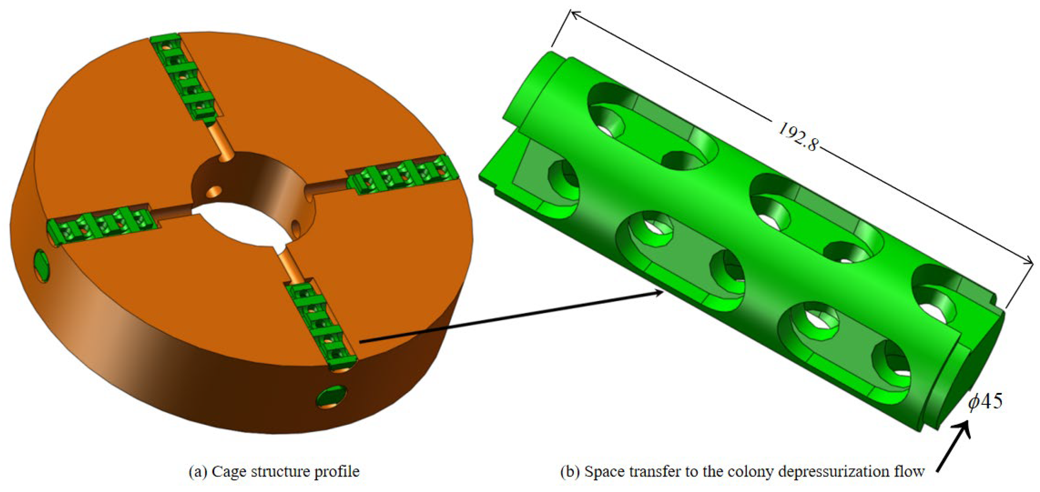
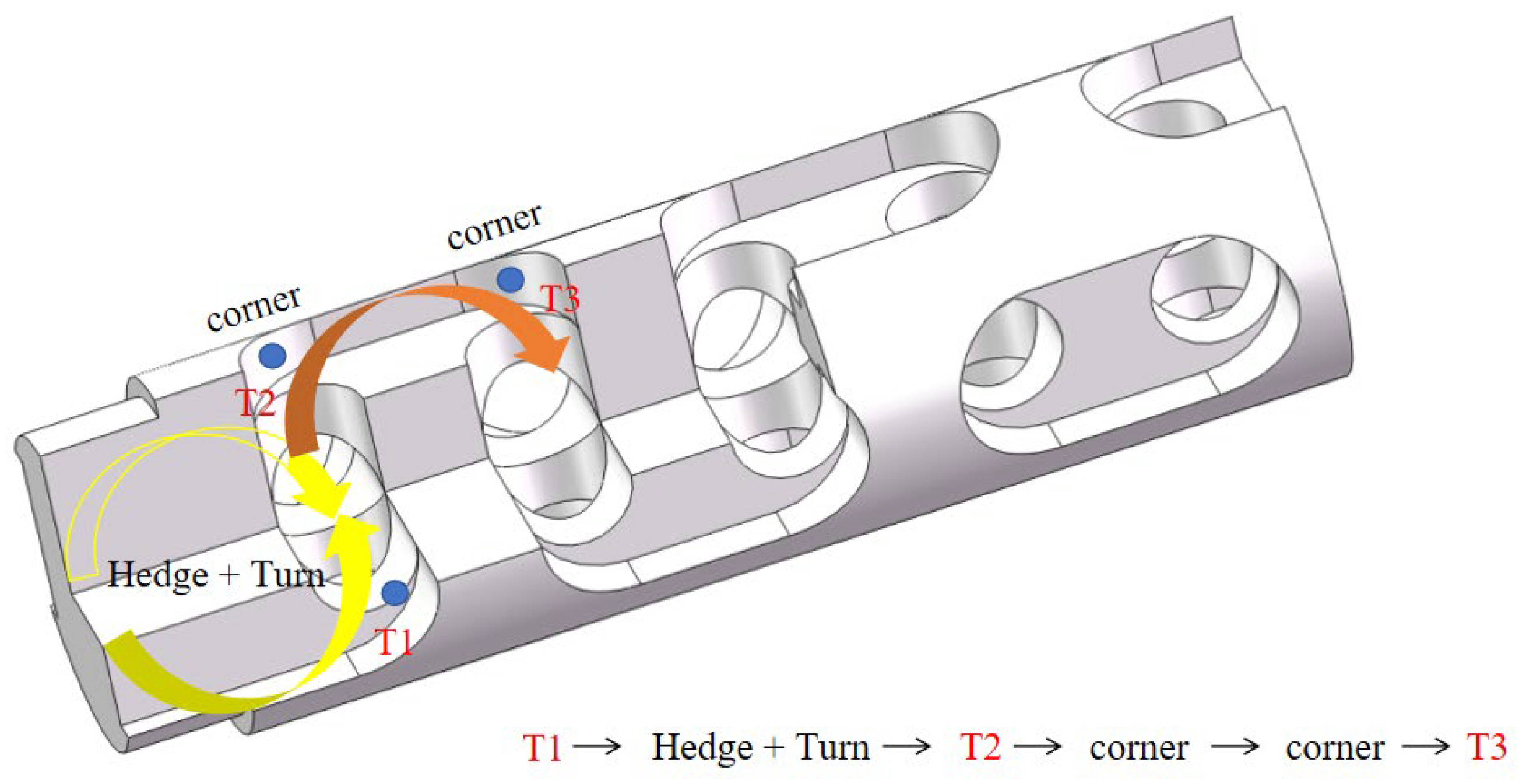
The structure of the pressure-reducing channel in the valve core examined in this study is illustrated in Figure 1, while Figure 2 provides a schematic diagram of the pressure-reducing process in the multi-stage flow channel. When high-pressure fluid enters the pressure-reducing flow channel from the outer barrel region of the valve core, it not only flows through various apertures and U-shaped grooves, altering its flow area and repeatedly changing direction, but also undergoes flow mass hedging. The pressure is distributed across multiple stages, with each throttling element sharing the load. This design ensures a smooth transition from critical pressure to working pressure, meeting the operational requirements for high-pressure differential parameters.
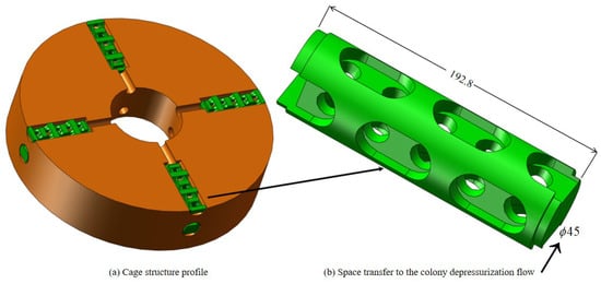
Figure 1.
Spool step-down runner structure.
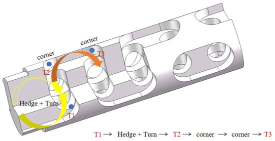
Figure 2.
Schematic diagram of the multi-stage offset flow channel pressure drop process.
In this study, the spatial transfer anthill pressure-reducing channel is investigated and analyzed independently, with its specific structure illustrated in Figure 1. The spool features an outer wall diameter of 45 mm and an overall length of 192.8 mm. Figure 2 provides a schematic representation of the pressure drop process within the multi-stage hedging channel. A bidirectional fluid–structure interaction (FSI) method is employed to discretize both the solid domain of the spool runner and the fluid domain of the flow channel, as depicted in Figure 3 and Figure 4.
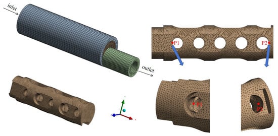
Figure 3.
Solid domain grid.
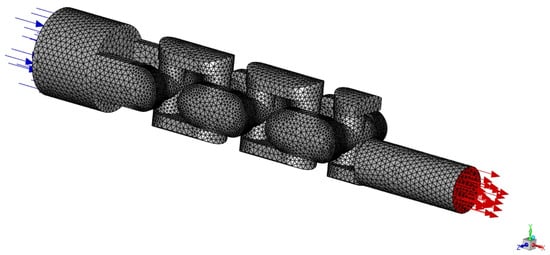
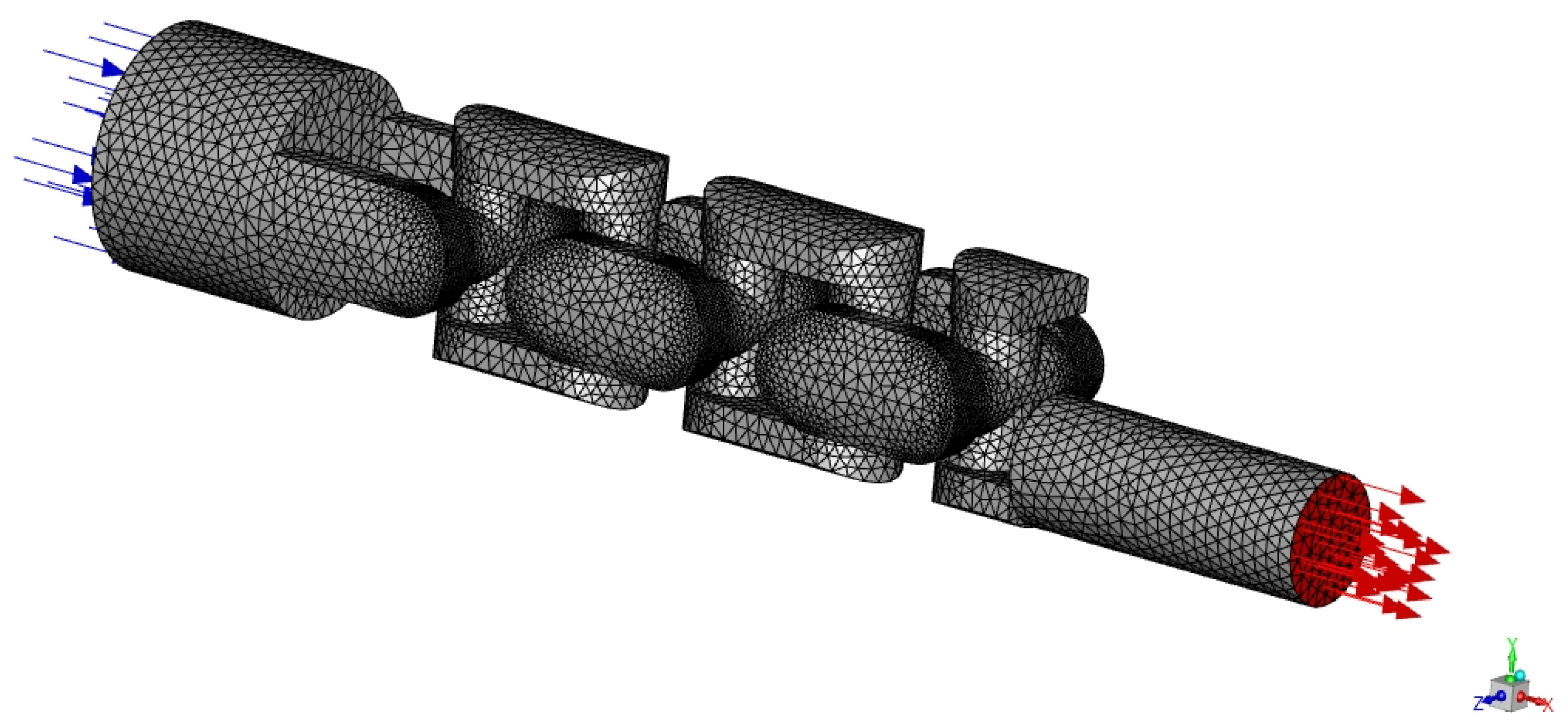
Figure 4.
Fluid domain grid.
The quality of the mesh significantly influences the accuracy of numerical simulations. Mesh generation is conducted using the Mesh platform. Given the complex geometry of the flow channel and the intricate nature of the internal flow field, discretization through scanning alone is insufficient. For both the fluid and solid domains, the polyhedral mesh method is employed to discretize the inlet and outlet outer cylinders as well as the valve core flow channel. This approach accommodates the complex structural features, reduces the total number of mesh elements, and enhances computational efficiency. The component size is set to 4 mm for the inlet and outlet outer cylinders and 2 mm for the spool flow channel, with local mesh refinement applied in critical areas, as illustrated in Figure 3.
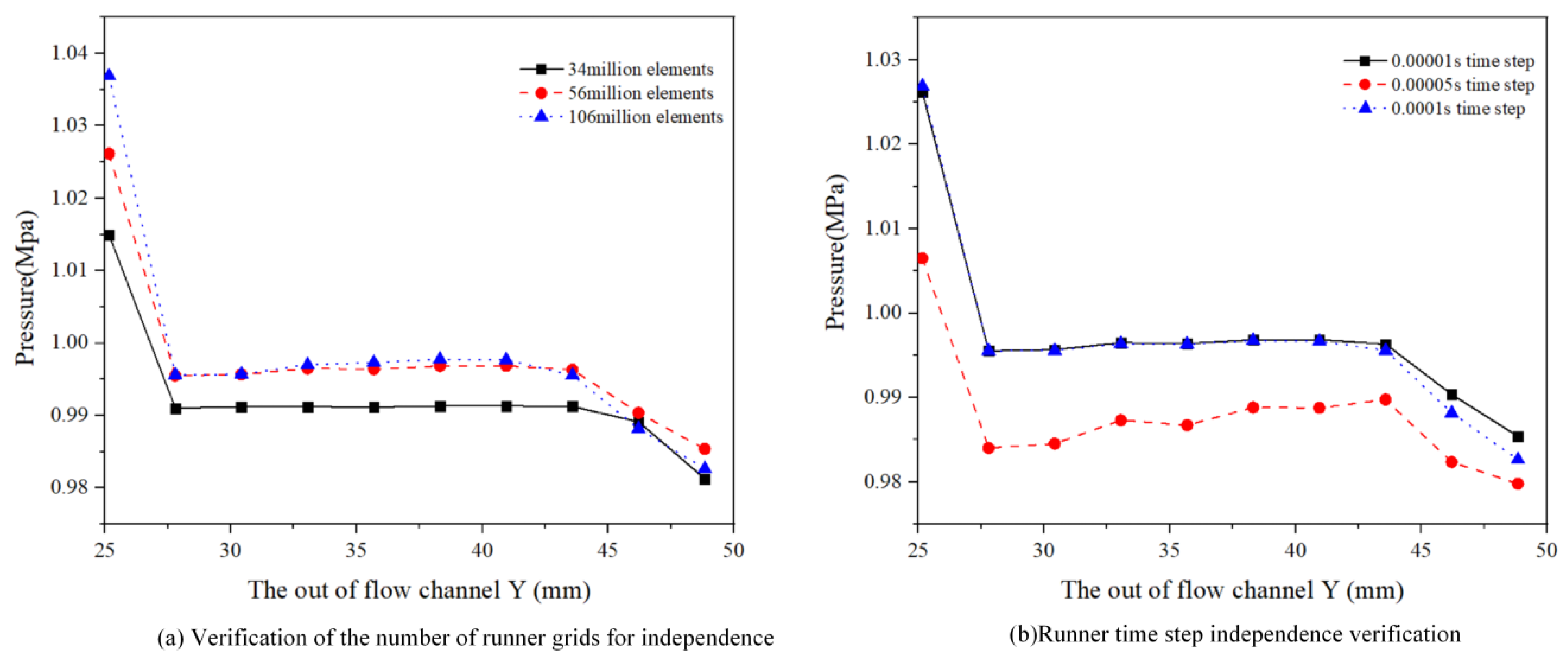
As illustrated in Figure 4, the watershed of a single pressure-reducing channel is extracted and subsequently meshed. The mesh is configured with a minimum size of 1 mm and a maximum size of 3 mm. To accurately capture the complex flow behavior at the watershed boundary, the flow channel boundary layer is set to 5 layers. Mesh generation for the single pressure-reducing channel is performed, and the sizing control values are adjusted to produce meshes with varying element counts. The outlet line pressure is calculated for mesh counts of 340,000, 560,000, and 1.06 million, respectively. As shown in Figure 5, when the mesh count reaches 560,000, the pressure trend at the outlet line of the flow channel stabilizes, and the pressure reduction value exhibits minimal variation. Therefore, a mesh count of 560,000 is selected for numerical simulations of the single pressure-reducing channel. To validate the independence of the results from the time step, three distinct time steps—0.00001 s, 0.00005 s, and 0.0001 s—were selected for simulation. Each simulation was conducted until a steady state was achieved. As illustrated in Figure 5b, the results reveal no significant differences in the trends across the three time steps, with the outcomes for 0.00001 s and 0.0001 s being nearly identical. However, the accuracy at 0.00005 s was slightly lower. Considering the extremely short duration of the flow channel vibration, a time step of 0.00001 s was identified as the optimal choice. As presented in Table 1, the maximum equivalent stress and stress strength of the solid domain mesh were calculated for the flow channel in the static structure at mesh sizes of 170,000, 290,000, and 560,000. The results demonstrate that when the mesh size exceeds 290,000, the deviations in equivalent stress and stress strength are 5.8% and 15.8%, respectively. In contrast, when the mesh size is below 290,000, the deviations are significantly reduced.
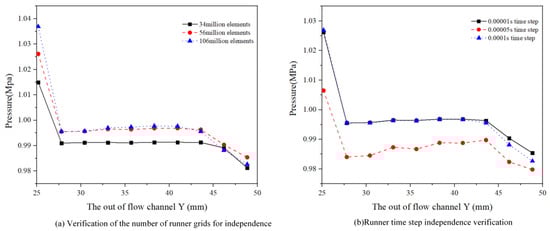
Figure 5.
Runner grid independence verification.

Table 1.
Solid domain grid independence verification.
2.2. Mathematical Model and Computational Model
2.2.1. Fluid Flow Mode
The flow analysis entails resolving the equations for unsteady, incompressible, turbulent flow, which are derived from the conservation laws of mass and momentum, employing the FLUENT in ANSYS 2020 R2.To comprehend the intricate dynamics and transfer mechanisms of turbulent flow within the valve and step-down channel systems, it is crucial to accurately capture and analyze the turbulent patterns in the complex and confined channel flows examined in this study. The realizable k-ε model, which operates under the assumption of Reynolds time averaging, is employed for this particular application. Within this conventional framework, two fundamental variables are computed, accompanied by their respective transport equations:
The following formula applies:
In the above formula, is the generation term of the turbulent kinetic energy caused by the average velocity gradient; is the generation term of the turbulent kinetic energy caused by buoyancy, for the incompressible fluid; ; is the dissipative term; is the compressibility correction term, and is the contribution of pulsation expansion in compressible turbulence. is the generated of the item; is the buoyancy correction term; is the dissipative term; and are the equation and the source term of the equation, respectively; is the speed of sound; is the coefficient of thermal expansion .
In the realizable k-epsilon model, the values of the empirical constants are as follows:
2.2.2. Fluid–Structure Coupling Model
For a structure, the equation of motion for its dynamic analysis is as follows:
Each representative meaning of the above formula is as follows: represents the inertial force, represents the damping force, represents the elastic force; the right side of the equation is used to represent the acting load, through the above formula, and the meaning of free vibration is added in the natural frequency; if the structure is not subject to external forces, and no damping occurs, then and .
Then its dynamic equation becomes as follows:
Fluid–structure interaction (FSI) occurs exclusively at the interface between the two phases, where the fluid and the solid structure share identical velocity and pressure conditions. These shared conditions serve as the boundary conditions for the fluid–structure interaction. By implementing this setup, we can more accurately model the FSI process, capturing the dynamic effects of the fluid on the structure as well as the feedback of structural deformation on the flow field. These boundary conditions play a pivotal role in the coupled analysis of fluid dynamics and structural dynamics, providing a robust theoretical foundation for our subsequent in-depth investigation of the flow field, lift forces, and vibration characteristics of the spool. The coupling in the governing equations is introduced through the equilibrium and compatibility conditions at the two-phase interface. The finite element method (FEM) is employed to solve the fluid–structure interaction problem. Specifically, the fluid domain and structural domain are discretized using FEM, and the boundary conditions are enforced during the assembly of the finite elements. Assuming is the variable increment of the coupled system, the simplified coupled vibration equation is obtained according to the different physical domains where the nodes are located:
where the following applies: and are, respectively, represented as the fluid domain and structural domain; and are represented as variables at the coupling interface and internal nodes, respectively; , is the equivalent mass matrix of the coupled system; are node unknown vectors in the fluid domain, coupling interface, and structure domain, respectively. are the external force vectors in the fluid domain, the coupling interface, and the structural domain.
FSI follows the most basic conservation principle. It satisfies the equality or conservation of the variables such as stress and displacement at the solid–liquid interface.
In the formula, the subscripts and represent the fluid and the solid, respectively. is the shear stress.
2.2.3. Boundary Conditions and Physical Parameters
For the boundary conditions of fluid calculations, the spool runner operates with a liquid water medium at 15 °C. The density and viscosity of liquid water are 997.0034 kg/m3 and 8.9004 × 10⁻⁴ kg/m·s, respectively. The inlet pressure is 30 MPa and the outlet pressure is 1 MPa. A significant pressure differential can induce cavitation, whereas a minor one might not cause perceptible vibrations. The operational settings accommodate both scenarios. The entire boundaries of the flow domain have been designated for system integration. The realizable k-epsilon model, renowned for its reliability, has been extensively utilized in engineering practices and serves as the foundation for our computations.
For the boundary conditions applied to the solid domain, the material of the spool flow channel is specified as YGB, while the inlet and outlet outer barrels are constructed from Structural Steel. The material properties are detailed in Table 2. Given that the components are rigidly connected, the contact relationship between them is defined as “binding”. The wall surface of the inlet outer cylinder is set as a fixed support to constrain its motion. The walls in contact with the fluid are designated as Fluid–Solid Interfaces to facilitate the coupling between the fluid and solid domains. All boundary condition settings and calculations are performed within the transient structural analysis module.
Table 2.
Material properties of the major components.
2.3. Numerical Method Verification
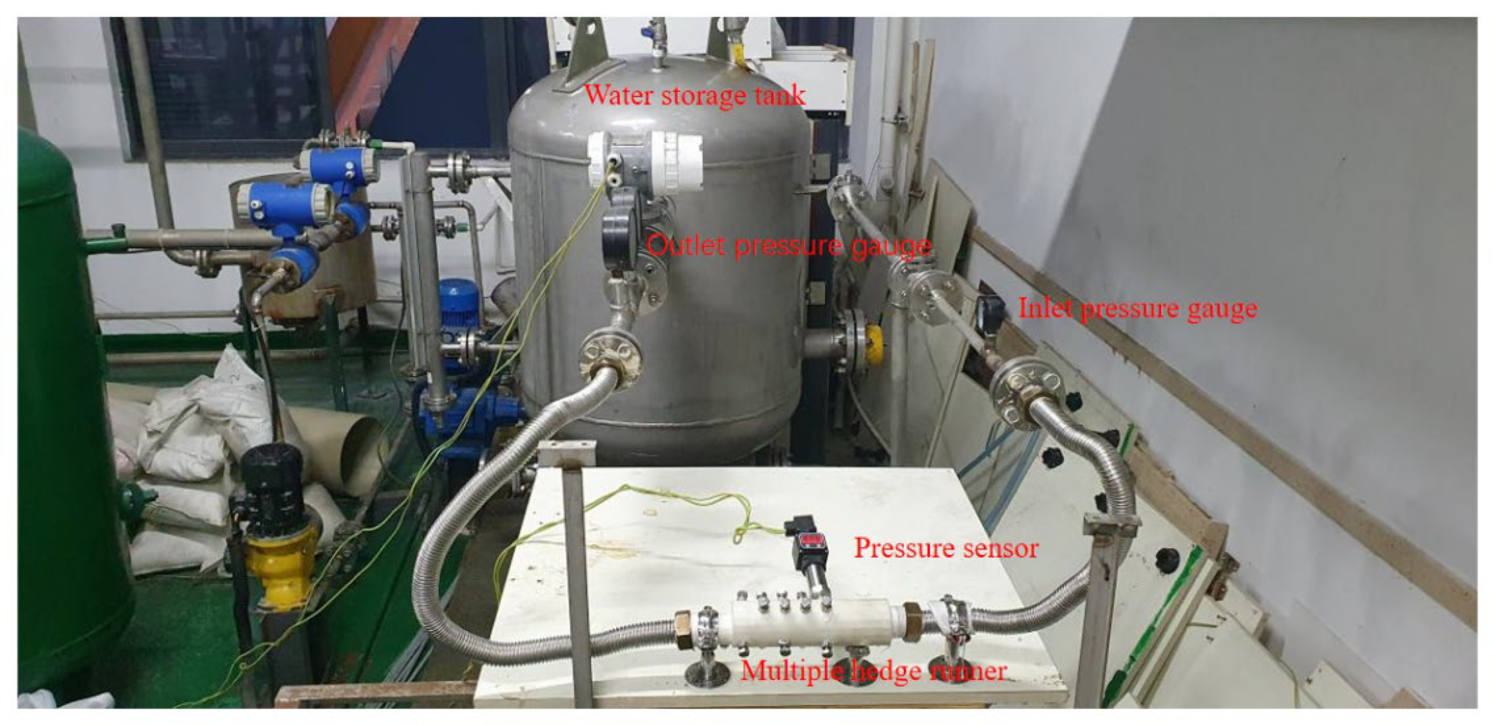
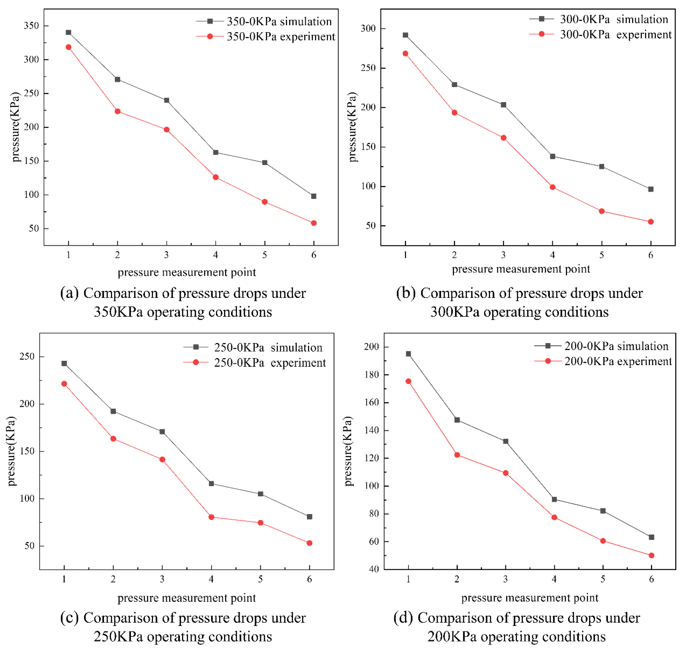
An experimental platform was constructed to establish a simplified numerical calculation model, as illustrated in Figure 6. Based on the operating range of the centrifugal pump (up to 500 kPa), four specific working conditions were designed: 350–0 kPa, 300–0 kPa, 250–0 kPa, and 200–0 kPa, where the inlet pressures were 350 kPa, 300 kPa, 250 kPa, and 200 kPa, respectively, and the outlet pressure was maintained at 0 kPa. The experimental results are presented in Figure 7. Pressure measurement points were selected at the first stage of the flow channel and the hedging stage, and the simulated and experimental pressure drop profiles under different working conditions were compared. The results demonstrate that, under all four conditions, the overall pressure decreases stepwise, and the pressure drop trends are consistent. This aligns with the multi-stage hedging and transfer design of the spatial transfer anthill flow channel, which achieves effective energy dissipation through hedging, transfer, and directional changes within the complex flow channel, thereby reducing the pressure of the high-pressure fluid. The simulated pressure values at the measurement points are higher than the experimental values. This discrepancy arises because the numerical calculations assume an ideal state for the fluid flow within the channel. In the experimental setup, the inlet pressure gauge is positioned above the flow channel and connected via flanges, pipes, and threads, which introduce significant hydraulic losses, including both frictional losses along the path and local losses at connections. These losses result in additional pressure reduction, creating a gap between the inlet pressure and the pressures at the measurement points. For example, under the 350 kPa condition, the error rate at measurement point 1 is 6.47%, the smallest among the six measurement points, while the error rate at measurement point 6 is the largest, reaching 42%. This larger error is attributed to the location of the final pressure measurement point, which is positioned directly above the outlet and adjacent to a closed blind plate. This configuration can cause back-flow and pressure instability. Both numerical simulations and experimental results confirm that the spool flow channel design effectively achieves multi-stage pressure reduction, with a significant pressure drop effect. The pressure drop trends observed in the simulations and experiments are in good agreement, validating the numerical simulation methods employing the mixture and realizable k-ε models for studying the internal flow characteristics of the spatial transfer anthill pressure-reducing valve. The experimental verification provides a robust foundation for the numerical calculations presented in this study.
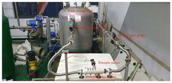
Figure 6.
Schematic diagram of the experimental apparatus.
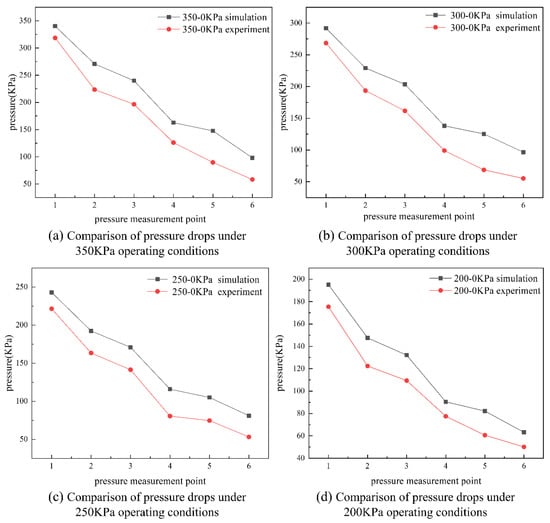
Figure 7.
Comparison of the pressure drop in simulation experiments under various operational conditions.
3. Results and Discussion
3.1. Spool Channel Flow Field
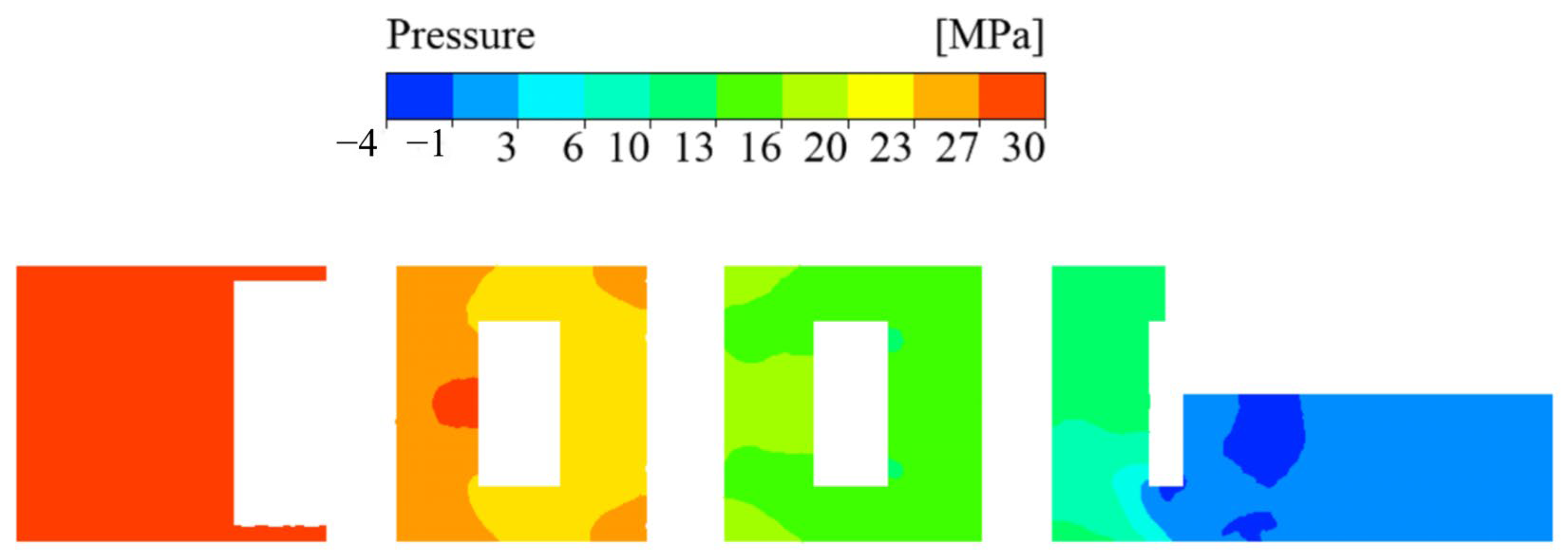
Flow characteristics are critical for fluid–structure coupling calculations, necessitating an initial evaluation of the flow field. Figure 8 illustrates the pressure distribution within the spool channel. Following the multi-stage pressure reduction process, the fluid pressure decreases progressively, with a significant pressure drop observed. High-pressure fluid is initially hedged at the front of each stage, then directed into a U-shaped groove, where it undergoes a change in direction before connecting to the subsequent stage. This process leads to a substantial reduction in fluid pressure. As the fluid passes through the impact walls at the U-shaped slots of the second and third stages and changes direction, the pressure decreases further due to the effective energy dissipation achieved through the angled geometry of these slots. The sequential hedging, turning, and redirection of the high-pressure fluid facilitate a gradual reduction from critical pressure to working pressure. Under typical operating conditions, which involve significant pressure differentials, a pronounced low-pressure zone forms at several locations, including the flow channel outlet, the convergence cavity of the valve core, and the diffusion cavity.

Figure 8.
Flow channel pressure distribution diagram.
The average velocity distribution within the spool runner is illustrated in Figure 9. Higher flow velocities are observed after the initial hedging of the fluid mass and at the outlet of the flow channel, which is consistent with the pressure field distribution. Compared to the flow velocity at the inlet, the velocities in the convergence cavity and the diffusion cavity are significantly higher. This indicates that the pressure is reduced to the working pressure while the velocity increases due to the multi-stage pressure-reducing flow channels of the valve core structure. Even after convergence and diffusion, the fluid maintains a considerable flow rate at the outlet. In terms of velocity magnitude, the maximum outlet velocity of the flow channel reaches 126 m/s. At this speed, the fluid can cause erosion at the outlet end of the valve core, potentially leading to thinning of the flow channel walls and damage to the valve core. Additionally, in the U-shaped groove section of the flow channel, the velocity near the wall surfaces is relatively low. This is because the fluid undergoes directional changes within this narrow region, experiencing energy dissipation at each corner of the U-shaped groove. This energy dissipation is not reflected as an increase in velocity but rather as turbulence and impact forces. Consequently, the fluid velocity near the U-shaped groove walls remains relatively low.
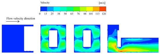
Figure 9.
Flow channel velocity profile.
The turbulent flow within the valve spool’s channel was analyzed. As shown in Figure 10, the fluid undergoes significant changes in velocity and direction as it enters the serpentine curves and offset channels, resulting in substantial mixing. This mixing process generates chaotic turbulence, which consumes energy, reduces pressure, and inhibits a rapid increase in flow rate. Additionally, vortices formed during this process may contribute to fluid-induced vibrations. Turbulence is particularly concentrated at the hedging centers and critical regions within the U-shaped grooves. Moreover, a notable increase in turbulence intensity is observed at the core of the valve, where the flow crosses the convergence point of the buck flow channels. This intensified turbulence is attributed to the vigorous mixing effect caused by the high flow rates.
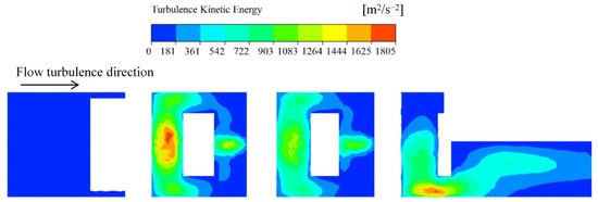
Figure 10.
Flow channel turbulence intensity distribution diagram.
3.2. Lift Analysis of Flow Field
When the fluid flows in the flow field, it exerts resistance on the downstream plane and generates lift perpendicular to the downstream plane. These forces are crucial for the interaction between the flow field and structure, leading to fluid-induced vibration. Drag and lift are primarily caused by vortex shedding in the flow field, which can be described using drag coefficient (Cd) and lift coefficient (CL).
In the formula, is the vortex-induced lift, is the vortex-induced drag, and is the cross-sectional area of the incoming flow.
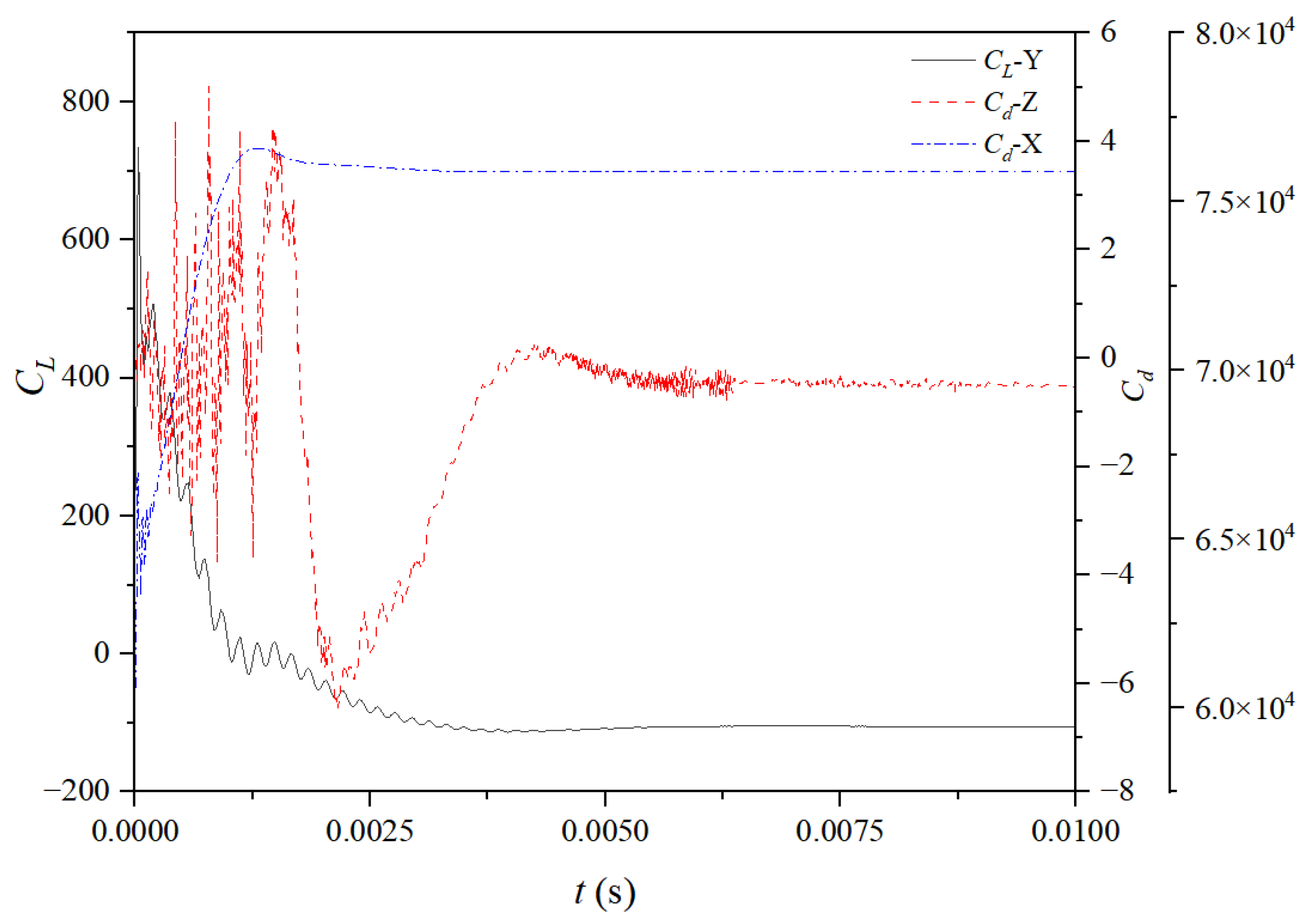
The flow direction within the spool flow channel determines the generation of the drag coefficient (Cd) along the X-axis and Z-axis, while the lift coefficient (CL) is generated along the Y-axis, as illustrated in the coordinate system of Figure 11. The variation in Cd-X values is particularly significant. Analysis of the flow field forces reveals that Cd along the X-axis initially peaks at 60,600, a value substantially higher than the force coefficients in the other two directions, and eventually stabilizes at approximately 75,893. This phenomenon can be attributed to the X-axis serving as the inlet for pressurized water, resulting in a significantly greater impact force compared to the other directions. The temporal variation curves of CL and Cd are depicted in Figure 11. In terms of magnitude, Cd-X, CL-Y, and Cd-Z differ by approximately one order of magnitude, indicating that the flow field force is greatest along the X-axis, followed by the Y-axis, and smallest along the Z-axis. Over time, CL-Y rapidly increases to a peak value of 735 from an initial instantaneous value of 236, then gradually decreases and stabilizes at around −108. The negative sign indicates that the fluid flows downward along the Y-axis. Initially, Cd-Z exhibits fluctuating positive and negative values, reaching a minimum of −6.33 at approximately 0.002 s, before increasing and stabilizing at around 0.21. During its initial phase, Cd-Z undergoes the most pronounced fluctuations in flow field force before ultimately stabilizing near −5.
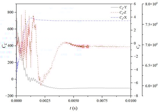
Figure 11.
Curve of CL and Cd with time.
To better understand the characteristics of the flow field lift, we further analyzed the trends of Cd-X, CL-Y, and Cd-Z and their relationship with the fluid flow state. The significant numerical fluctuations of Cd-X in the initial stage may be attributed to the sudden changes in the shape and structure of the valve core as the fluid enters the spool flow channel, leading to instability in the fluid flow state and generating a large impact force. The trend of CL-Y reflects the dynamic response of the fluid in the Y-axis direction. The high instantaneous value observed initially may result from the fluid being obstructed by the spool in the Y-axis direction, producing a substantial lift force. As the fluid continues to flow, CL-Y gradually increases to a maximum value, then decreases and eventually stabilizes around a negative value. This indicates that the fluid experiences a continuous downward force in the Y-axis direction, consistent with the observed downward flow of the fluid along the Y-axis. The variation in Cd-Z is more complex, with initial fluctuations between positive and negative values likely caused by the influence of the valve core’s shape and the flow channel’s structure on the fluid in the Z-axis direction, leading to an unstable flow state. As the fluid continues to flow, Cd-Z gradually increases and stabilizes around a specific value. Although the magnitude of Cd-Z is relatively small, its variation still reflects the forces acting on the fluid in the Z-axis direction.
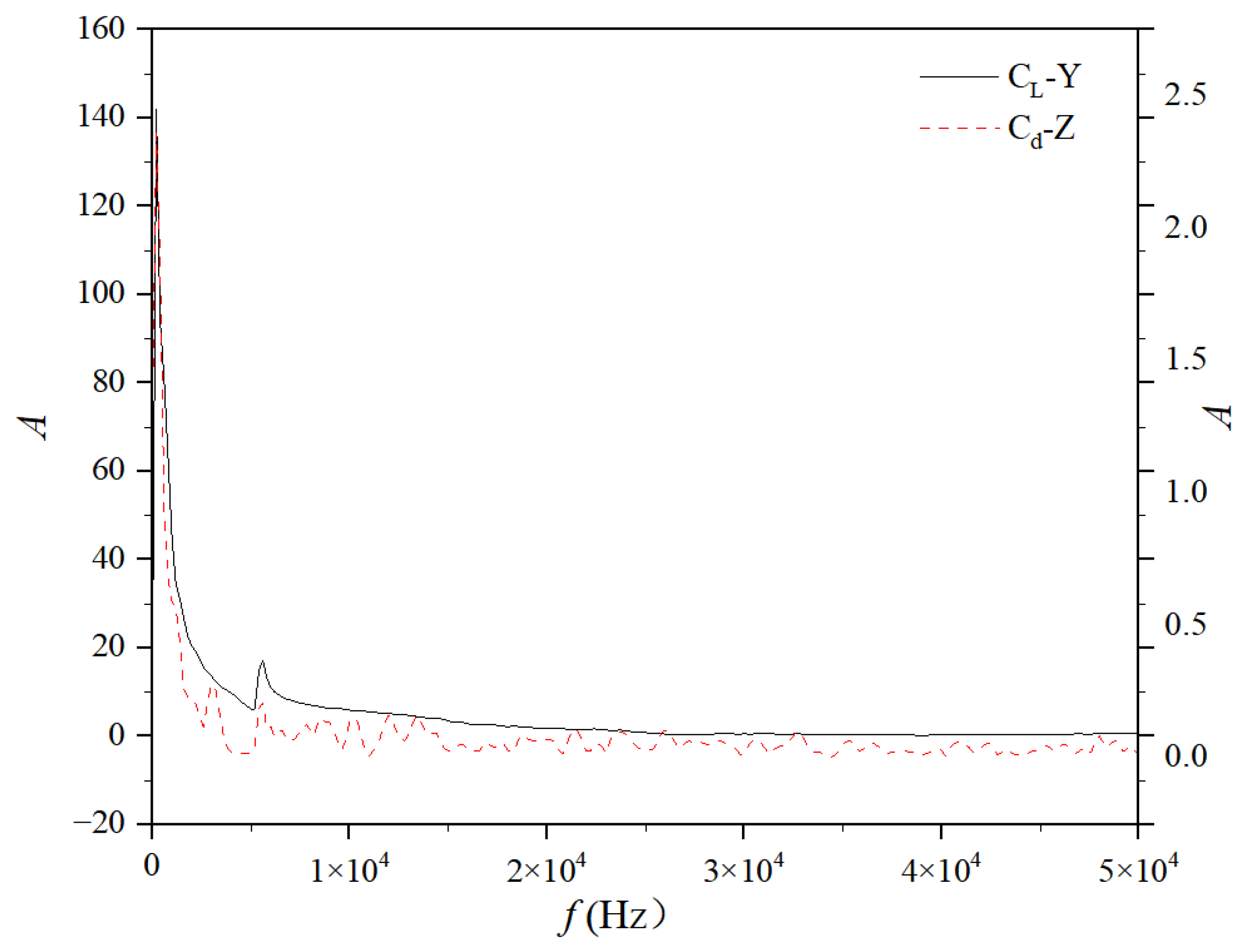
The time domain data for the spinner flow channels CL-Y and Cd-Z are converted using a fast Fourier transform (FFT), as illustrated in Figure 12 below. It is evident that, throughout the majority of the frequency spectrum, the fluctuations are largely alike, with sharp peaks at the beginning and a subsequent gradual decline, accompanied by a secondary peak at approximately 5400 Hz, which corresponds to the vortex shedding frequency range. The amplitude fluctuations of Cd are markedly greater than those of CL, suggesting a more vigorous flow field force along the Z-axis of the spinner flow path in contrast to the Y-axis, and exhibiting less instability than on the Y-axis.
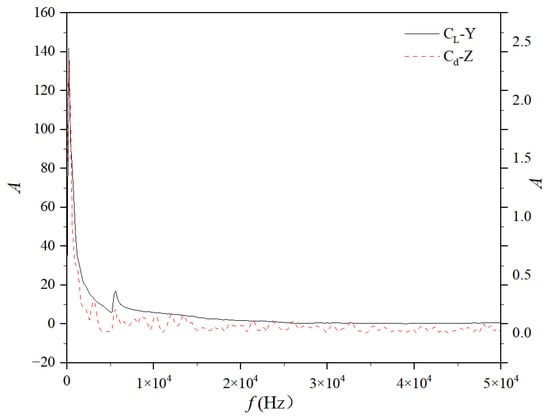
Figure 12.
Flow channel CL, Cd spectrum diagram.
3.3. Spool Vibration Analysis
Fluid-induced vibration refers to the varying excitations caused by the interaction between structural surfaces of process components and the surrounding fluid or the internal flow of the fluid. These excitations generate specific magnitudes of response within the process components, leading to corresponding structural vibrations. In this study, the configuration of the multi-stage pressure-reducing flow channel is examined under high-pressure differential conditions. A two-way fluid–structure coupling method is employed to investigate and analyze the vibrational behavior of the pressure-reducing flow channels.
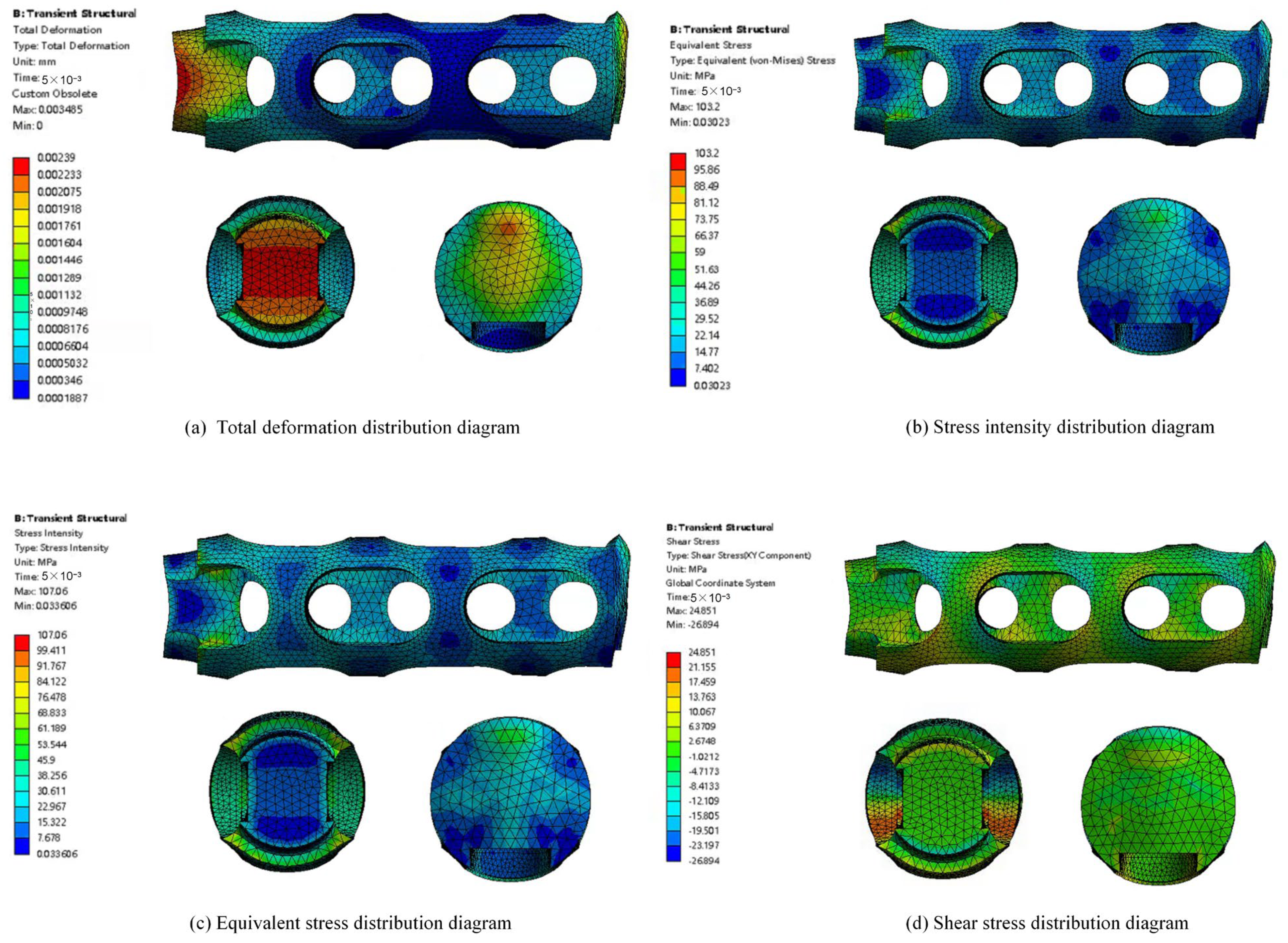
The solution induces deformation in a single flow channel under a pressure range of 30–1 MPa across its boundary domain. The deformation scale factor of the runner is 3.5 × 10³ (auto-scaling). The resulting distribution diagrams, illustrating the equivalent stress, shear stress, and stress intensity generated by the U-shaped groove, are presented in Figure 13. The analysis of the three surfaces in Figure 13a reveals that the flow channel experiences its maximum deformation (0.0034 mm) at the inlet surface of the high-pressure flow. Significant deformation also occurs during the initial stage of pressure reduction and at the terminal stage of the outlet. The substantial deformation observed in the initial phase is attributed to the positive hedging of the high-pressure medium, while at the terminal stage, it results from structural thinness, leading to pronounced deformation. The stress intensity under normal operating conditions is depicted in Figure 13b, with a peak value of 107 MPa observed at the corner edge of the U-shaped slot between the primary and secondary hedges. This value is significantly lower than the allowable stress for the YG8 material used in the flow channels. Overall, the stress intensity distribution is relatively dispersed, with large values still present at the entrance and exit ends, contributing to significant flow channel deformation. Considering the impact of shear force on the flow channels, Figure 13c illustrates the shear stress distribution, showing a peak value of 24.8 MPa at the inlets of the first and second stages of the U-shaped grooves. Notably, significant shear stresses are concentrated at the corners where fluid exits from the upper stages via the U-shaped grooves into subsequent stages. This indicates that, for an individual flow channel, shear force damage primarily manifests as corner impacts caused by high-pressure fluid within the U-shaped grooves. The equivalent stress distribution within a single pressure-reducing flow channel is depicted in Figure 13d. The location of peak equivalent stress coincides with that of maximum stress intensity, reaching approximately 103.2 MPa, which differs by about 4.2 MPa from the stress intensity peak. The analysis suggests that structural damage is predominantly caused by normal stress, while the flow channel’s damage results from the combined effects of normal and shear stresses, particularly at the corners of the U-shaped slots, where shear forces exert a more significant influence.

Figure 13.
Flow channel parameter distribution diagram.
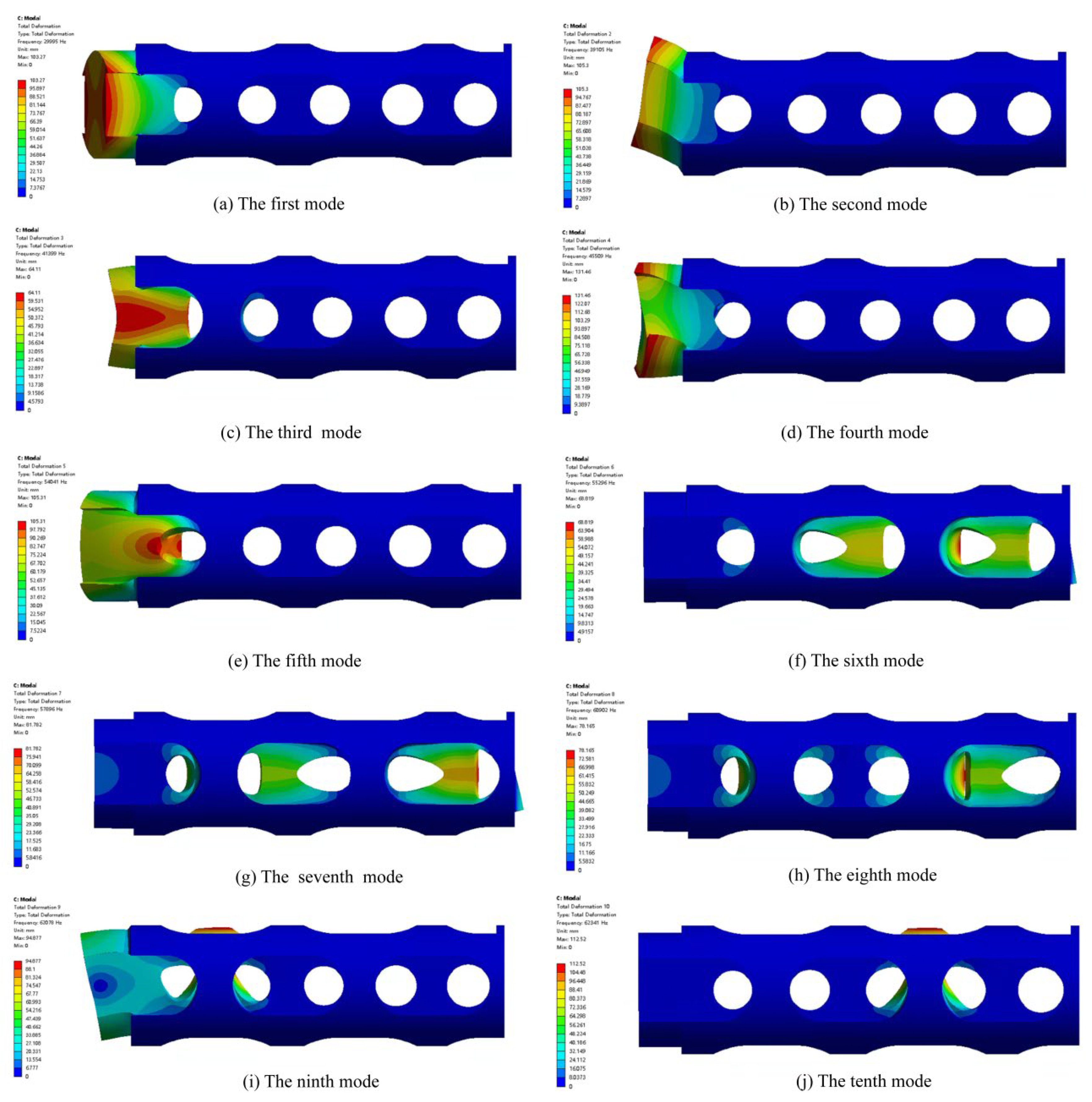
Modal analysis of the statically pre-stressed structure is conducted by calculating the solution for the tenth-order mode. The deformation diagram in Figure 14 illustrates the tenth-order mode of the flow channel. It is evident that significant deformation occurs at the entrance for the first- through fourth-order modes. Specifically, the first-, second-, and third-order modes exhibit displacement along the Z, Y, and X axes of the entrance segment, respectively, while the fourth mode demonstrates torsional bending with substantial deformation. The fifth mode’s deformation primarily affects the structure of the initial hedge channel. The sixth mode’s deformation is concentrated at the intersection of the third and fourth hedge regions. The remaining modes each exhibit distinct locations of maximum deformation. These deformation locations align with areas of high-pressure fluid impact and shear stress concentration within the flow channel, further confirming the strong correlation between flow channel damage and hydrodynamic properties. Specifically, when high-pressure fluid passes through the corners of the U-shaped grooves, the flow channel structure becomes more susceptible to deformation due to the influence of shear stress. Additionally, the modal shape deformation diagram reveals that deformation gradually extends from the inlet position toward the interior of the flow channel as the modal order increases. This phenomenon may be related to the flow velocity and pressure distribution of the fluid within the channel. Therefore, the impact of hydrodynamic characteristics on structural deformation must be thoroughly considered during the design of the spool flow channel. This approach will enable optimization of the flow channel structure, enhancing the stability and durability of the spool.

Figure 14.
Flow channel 10 mode diagram.
The modal resonance frequencies of individual flow channels are analyzed, as shown in Table 3 below. Initially, the natural frequencies of a single flow channel are calculated. It is observed that the first six natural frequencies are very small, nearly approaching zero, in the case of an unconstrained flow channel. These first six modes correspond to rigid body modes, where the vibration patterns resemble rigid body motion. Specifically, the first two modes exhibit no distortion or deformation, while the third, fourth, fifth, and sixth modes involve bending deformation. Beyond the sixth mode, the natural frequency of the seventh mode rises to 1386 Hz and continues to increase progressively up to the tenth mode. The seventh mode’s unconstrained natural frequency increases significantly to 5888 Hz, with the increment growing larger as the mode order increases. By the tenth mode, the natural frequency reaches 11,603 Hz, falling within the high-frequency range.
Table 3.
The first ten natural frequencies and modal frequencies of a single multi-stage hedge runner.
In practical operation, the flow channel is embedded within the spool structure and forms a fit with the cage sleeve, introducing constraints. To account for this, constraint surfaces are applied to the outer wall and end interfaces between the flow channel and the sleeve. The resulting natural frequencies under constraint are summarized in the table below. The constrained natural frequencies show a smaller variation compared to the unconstrained case, with the sixth-order constrained natural frequency being similar to the seventh-order unconstrained natural frequency. Under these constraints, the natural frequencies exhibit significant changes, particularly for the first six modes, while the higher modes (7th to 10th) show relatively minor variations. Overall, the natural frequencies increase from 28,602 Hz in the first mode to 59,069 Hz in the tenth mode. The frequencies of the flow-induced vibration modes, incorporating static structural pre-stress, are also presented in the table. The results indicate that the modal frequencies are close to the constrained natural frequencies, with differences ranging between 1000 and 3000 Hz for each mode. This suggests that the resonance response due to flow-induced vibration is more pronounced and densely distributed compared to that of the entire valve under a single flow channel. In the first six modes, the second-order modal frequency aligns closely with the third-order constrained natural frequency, while the third-order modal frequency corresponds to the fourth-order constrained natural frequency. This implies that, for a single flow channel, the resonance response frequency range caused by flow-induced vibration lies between 39,000 Hz and 41,000 Hz, falling within the high-frequency range. The resonance primarily manifests as simple harmonic motion along two or three orthogonal directions, predominantly affecting the deformation and damage at the inlet section of the flow channel.
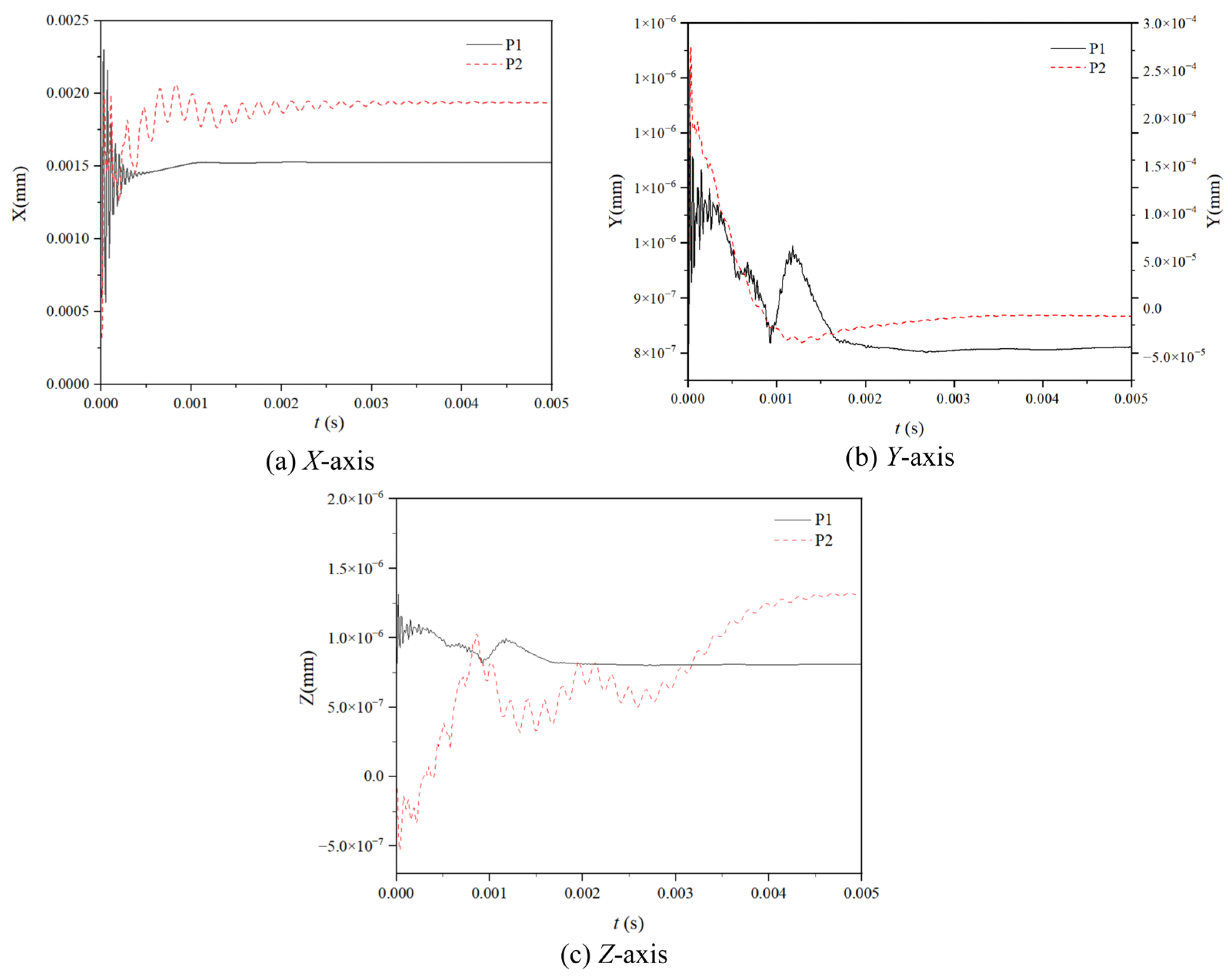
Two vibration monitoring points, designated as P1 and P2, are strategically positioned as illustrated in Figure 3, at the center of the primary corner and the midpoint of the final corner of the flow channel spool, respectively. The time-dependent vibration displacement curves for these two measurement points across the three axes are depicted in Figure 15. Each point exhibits distinct variation patterns across all three dimensions, with noticeable differences in amplitude and behavior. The amplitude of the vibrational displacement follows a consistent trend with the flow field force, peaking along the X-axis, reaching its lowest value along the Z-axis, and assuming an intermediate value along the Y-axis. Notably, there is a significant difference in the vibrational displacements between the two monitoring points along the Y-axis. The initial temporal fluctuation of P1 exceeds that of P2 across all three spatial dimensions, particularly during the initial phase when the spool flow path is opened and the vibration intensity reaches its maximum. On the X-axis, P1 stabilizes more quickly than P2, which exhibits a steady sinusoidal oscillation before eventually reaching equilibrium. The peak displacement of P2’s vibration is slightly greater than that of P1, a phenomenon attributed to structural changes in the terminal phase of the spool flow path. A sudden decrease in pressure coupled with an increase in flow rate leads to an amplification of the vibration amplitude. In the Y-axis direction, there is a notably large displacement disparity between the two measurement points. Analysis using a biaxial diagram reveals that although P1 experiences less displacement than P2, its fluctuation is more pronounced. In the Z-axis direction, P2 initially displays negative displacement, which gradually increases over time before stabilizing. This pattern indicates that a longer period is required for P2 to stabilize along the Z-axis, consistent with the previously described flow field forces.
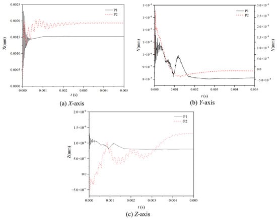
Figure 15.
Vibration displacement curves of two measuring points in different directions with time.
In summary, the analysis of the vibration displacement curves at two monitoring points across three directions provides fundamental insights into the vibration characteristics of the spool. These characteristics are crucial for a deeper understanding of the flow properties within the spool and for guiding its design optimization. Future research should focus on investigating the variation patterns of spool vibration under different operating conditions and exploring design strategies to reduce vibration amplitudes. Such efforts will enhance the stability and reliability of the valve, contributing to improved performance and longevity.
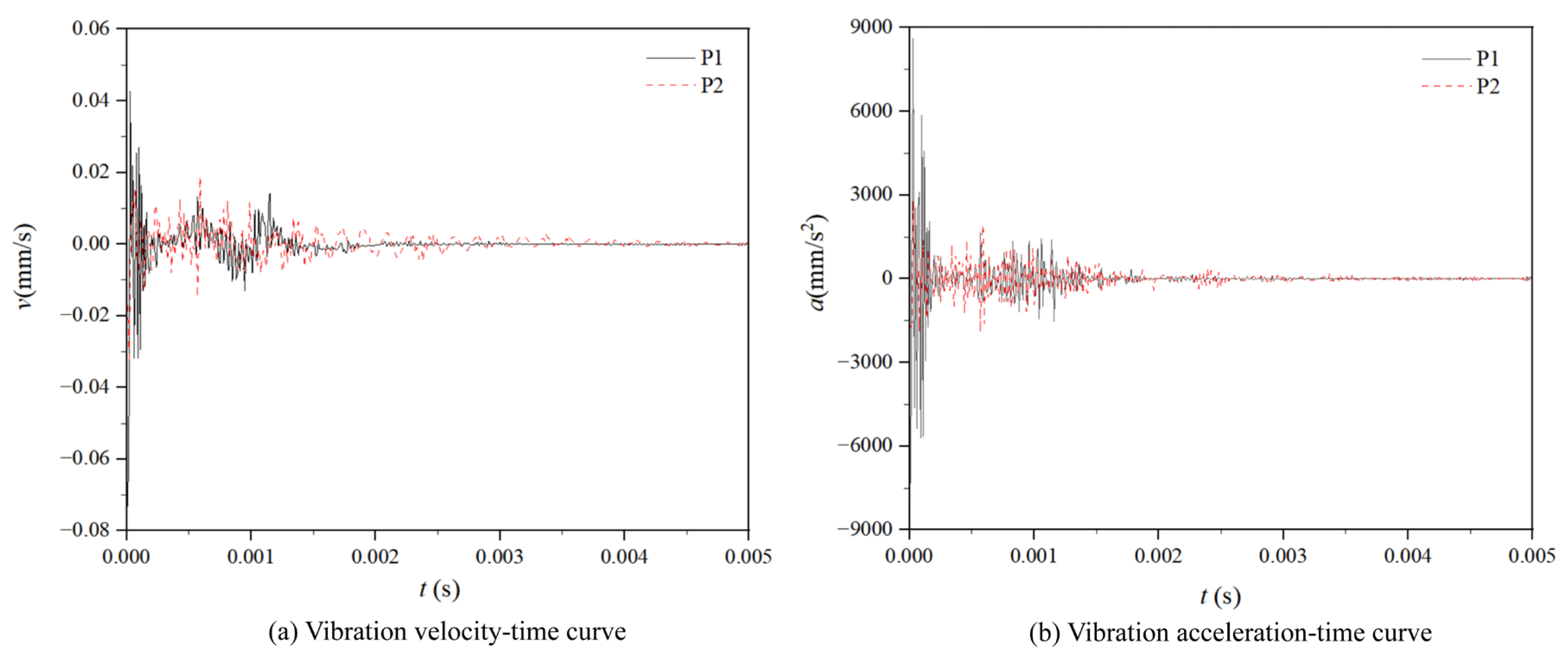
The time-domain data for vibration displacement is extracted and converted into corresponding time-domain data for vibration velocity and acceleration. The velocity and acceleration profiles along the Z-axis over time are illustrated in Figure 16. As shown in the figure, measuring point 1 achieves a peak vibration velocity of 4.27 × 10⁻² mm/s and a peak acceleration of 8621.5 mm/s2, while measuring point 2 reaches 1.19 × 10⁻² mm/s and 2772.4 mm/s2, respectively. The peak values at measuring point 1 are approximately three times those at measuring point 2. The vibration acceleration at the two measurement points stabilizes at 71.9 m/s2 and 24.3 m/s2, respectively. During the initial 0.003 s, intense vibrations occur, characterized by large alternating positive and negative velocities and accelerations. Subsequently, the vibration velocity decreases but continues to exhibit fluctuations. In terms of acceleration, a peak value of 8621 mm/s2 is observed during the rigid channel flow phase, posing significant challenges for vibration protection and potentially impacting the effectiveness of liquid pressure reduction. As depicted in Figure 17, the time-domain data for vibration acceleration in each direction is transformed using fast Fourier transform (FFT) to generate the corresponding vibration acceleration spectrum.
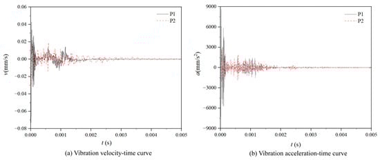
Figure 16.
The curve of vibration velocity and vibration acceleration of two measuring points in the direction of the Z-axis with time.
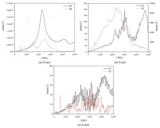
Figure 17.
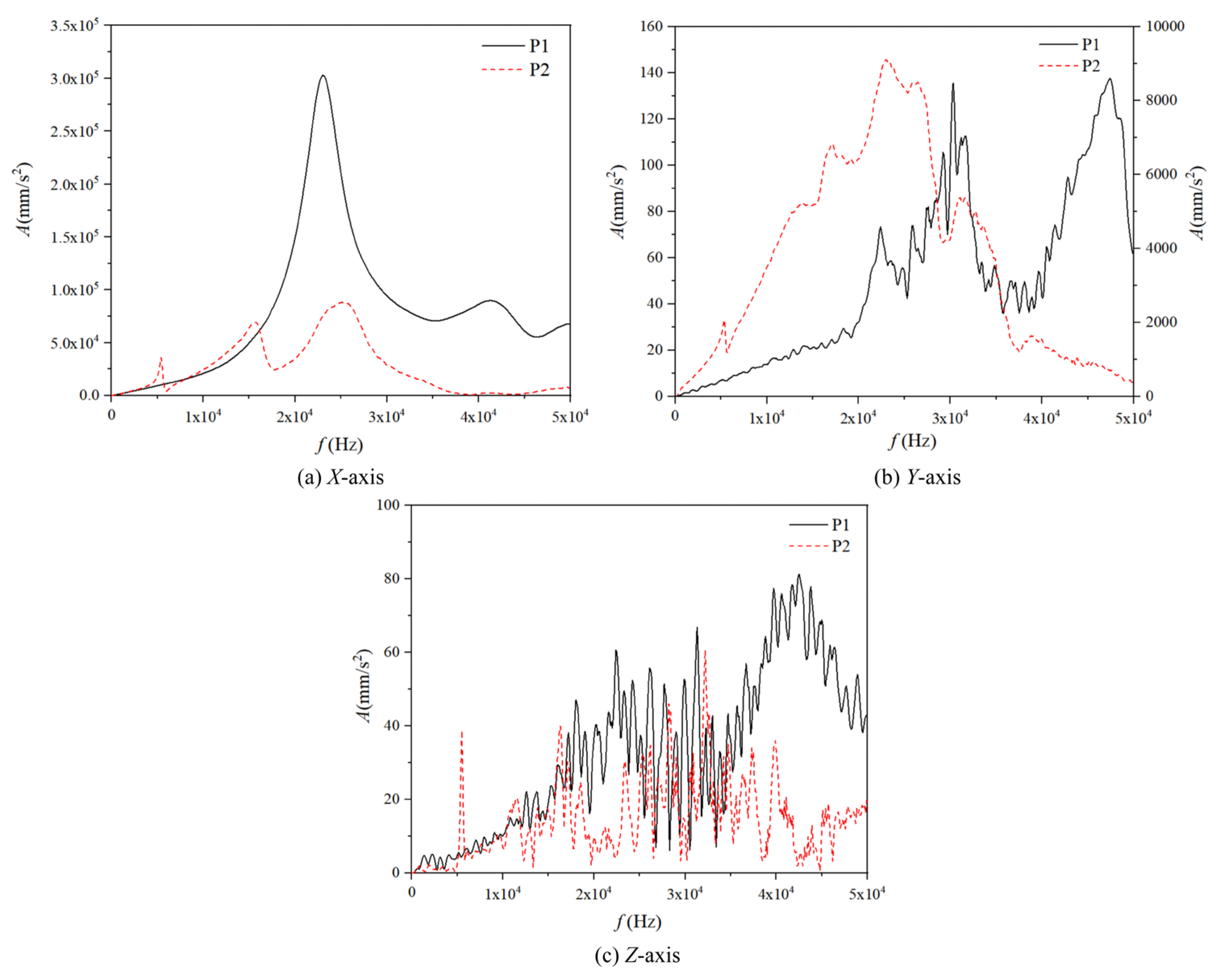
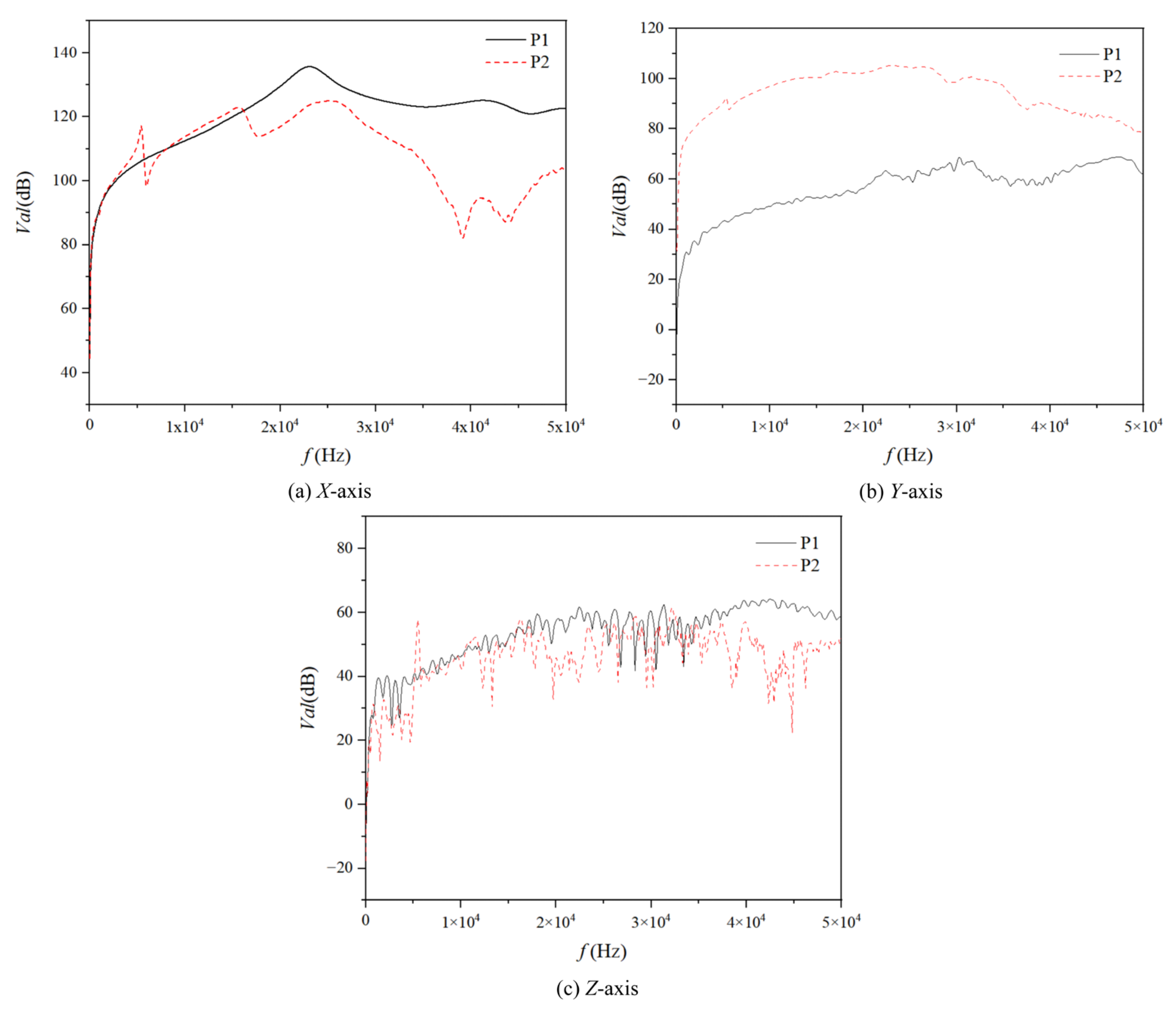
Vibration acceleration spectrum curves of two measuring points in different directions.
The characteristic curves of the vibration spectra at the two measurement points exhibit significant differences across the three axes, as illustrated in the figure above. Specifically, along the X-axis, P1 experiences vibrations primarily within the range of 20,000 to 45,000 Hz, with vibration acceleration levels fluctuating between 3.5 × 10³ and 5 × 105 mm/s2. Notably, peak accelerations occur at frequencies of 23,000 Hz and 41,800 Hz. In contrast, P2’s vibrations range between 5000 and 30,000 Hz, with a maximum peak acceleration of 8.8 × 104 mm/s2. Along the Y-axis, a significant difference in amplitude is observed between the two measurement points. At P1, pronounced vibrations occur within the range of 20,000 to 50,000 Hz, featuring multiple peaks. The maximum peaks at 30,400 Hz and 47,400 Hz approach accelerations of approximately 270 mm/s2. In contrast, P2 exhibits higher acceleration levels but less frequent variations in vibration amplitude due to its proximity to the flow channel outlet, where low-pressure fluid flows at high velocities. Along the Z-axis, the acceleration amplitudes at both measurement points are notably smaller than those in the X and Y axes. However, both points exhibit sharp changes in the Z-direction with multiple peaks. The main vibration amplitude of P1 on the Z-axis is similar to that on the Y-axis, reaching a maximum peak acceleration of 78 mm/s2. P2, however, shows different characteristics in the Z-direction, with multiple peaks and lower accelerations. The vibration range for P2 is 0–5000 Hz, with a maximum acceleration amplitude of 60 mm/s2. Furthermore, a comparison of the frequencies in Figure 14 with those listed in Table 2 reveals that the peak points correspond to the frequencies of the first, third, and fourth modes. The peak vibration positions for these modes are located at the inlet of the flow channel, aligning perfectly with the simulation results obtained from two-way fluid–structure coupling. This demonstrates that modal analysis plays a crucial role in guiding research on the characteristics of fluid-induced vibrations.
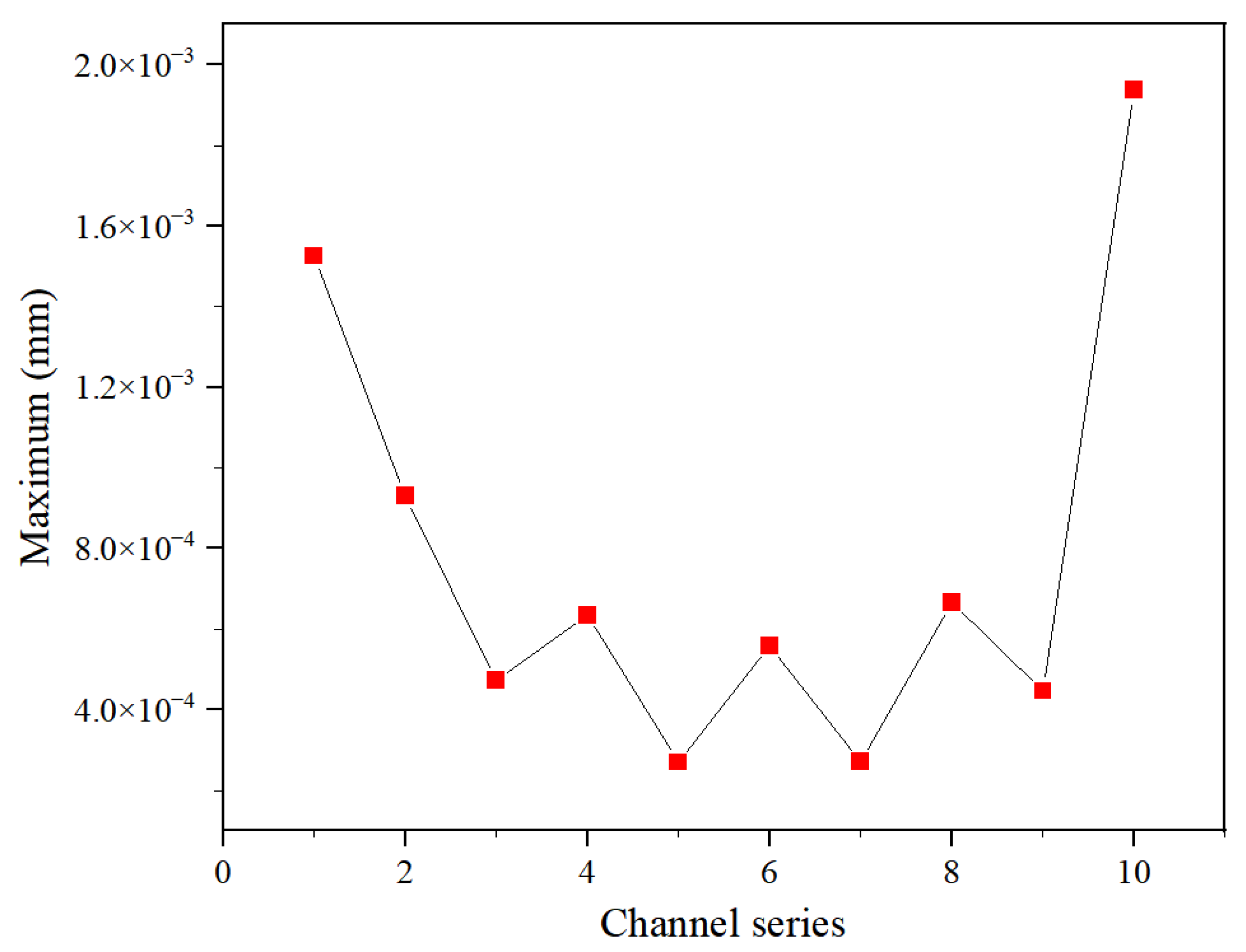
The peak deformation at the center of each stage’s groove surface within the flow channel is calculated, as illustrated in Figure 18 below. It is evident that the initial and concluding stages experience the most significant deformations, with values of 0.00153 mm and 0.00194 mm, respectively. In contrast, the deformations in the intermediate stages are all below 0.001 mm, with the least deformation occurring at the fifth and seventh stages, reaching a maximum of approximately 2.7034 × 10⁻⁴ mm. Upon entering the primary flow channel, the peak vibrational deformation progressively diminishes from stage 2 to stage 3, then increases until it peaks at stage 5, passing through stage 4, which corresponds to a bend in the flow channel. This is followed by a consistent pattern of deformation at each subsequent bend. The pressure-reducing mechanism within the spool flow channel causes a reduction in fluid pressure at each bend, thereby decreasing vibration levels. However, as the flow progresses and passes through these bends, vibration intensifies, with maximum deformation corresponding to changes in flow velocity and pressure. As the flow approaches the outlet of the final stage, where pressure is at its lowest due to structural constraints and high flow rates, intense vibrations occur, resulting in a sudden increase in deformation. To mitigate vibration-induced damage, it is essential to optimize the flow path design, particularly in areas prone to vortex shedding, to prevent such damage.
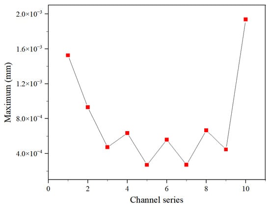
Figure 18.
The maximum deformation at the midpoint of each stage of the flow channel.
The degree of vibration at each stage can be determined with greater precision by measuring the total vibration acceleration level for each stage and transforming the vibration acceleration data from the time domain into the frequency domain. The calculation method for the vibration acceleration level is detailed in the equation provided below as Equation (9):
In the formula, Val refers to the vibration acceleration level, a refers to the vibration acceleration at each frequency, and a0 refers to the reference vibration acceleration, taking a0 as 10−3 mm/s2.
The spectrum diagram in Figure 19 illustrates the vibration acceleration levels at measurement points 1 and 2 across the three axes. It is evident that the vibration acceleration levels along the X-axis are notably high for both points, exceeding 60 dB, with point 1 consistently recording higher levels than point 2. This observation aligns with prior findings. Furthermore, the vibration acceleration levels at point 2 along the Y-axis consistently exceed those at point 1, fluctuating around and above 95 dB. In contrast, point 1 exhibits a gradual increase in vibration acceleration levels along the other two axes, reaching approximately 60 dB. In summary, the vibration acceleration levels at both measurement points are similar in magnitude along the Z-axis.
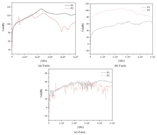
Figure 19.
Spectrum curves of vibration acceleration levels at two measuring points in different directions.
Further analysis of the spectrogram reveals distinct characteristics in the vibration acceleration levels across the three axes. In the X-direction, the spectrograms of both measurement points exhibit pronounced peaks in the high-frequency range, which may correspond to specific hydrodynamic excitation frequencies. In the Y-direction, although the vibration acceleration levels are relatively low, the spectrogram of measurement point 2 shows a continuous distribution within a certain frequency band, suggesting the presence of a relatively stable fluid excitation in this range. In the Z-direction, the spectrograms of both measurement points display significant variations, reflecting the complex flow characteristics of the fluid along this axis. Additionally, the vibration acceleration level at measurement point 1 gradually increases to approximately 60 dB, indicating that fluid excitation in the Z-direction intensifies as the flow progresses.
The vibration acceleration stage synthesis formula is employed to superimpose the vibration acceleration stages at varying frequencies, thereby calculating the aggregate vibration level at the central point of each stage within the spool flow channel, as depicted in Figure 18 below. The formula for synthesizing the total vibration level is presented in Equation (10):
In the formula, Valtotal refers to total vibration level, ni refers to the i sampling frequency vibration acceleration level, and N refers to number of frequency samples.
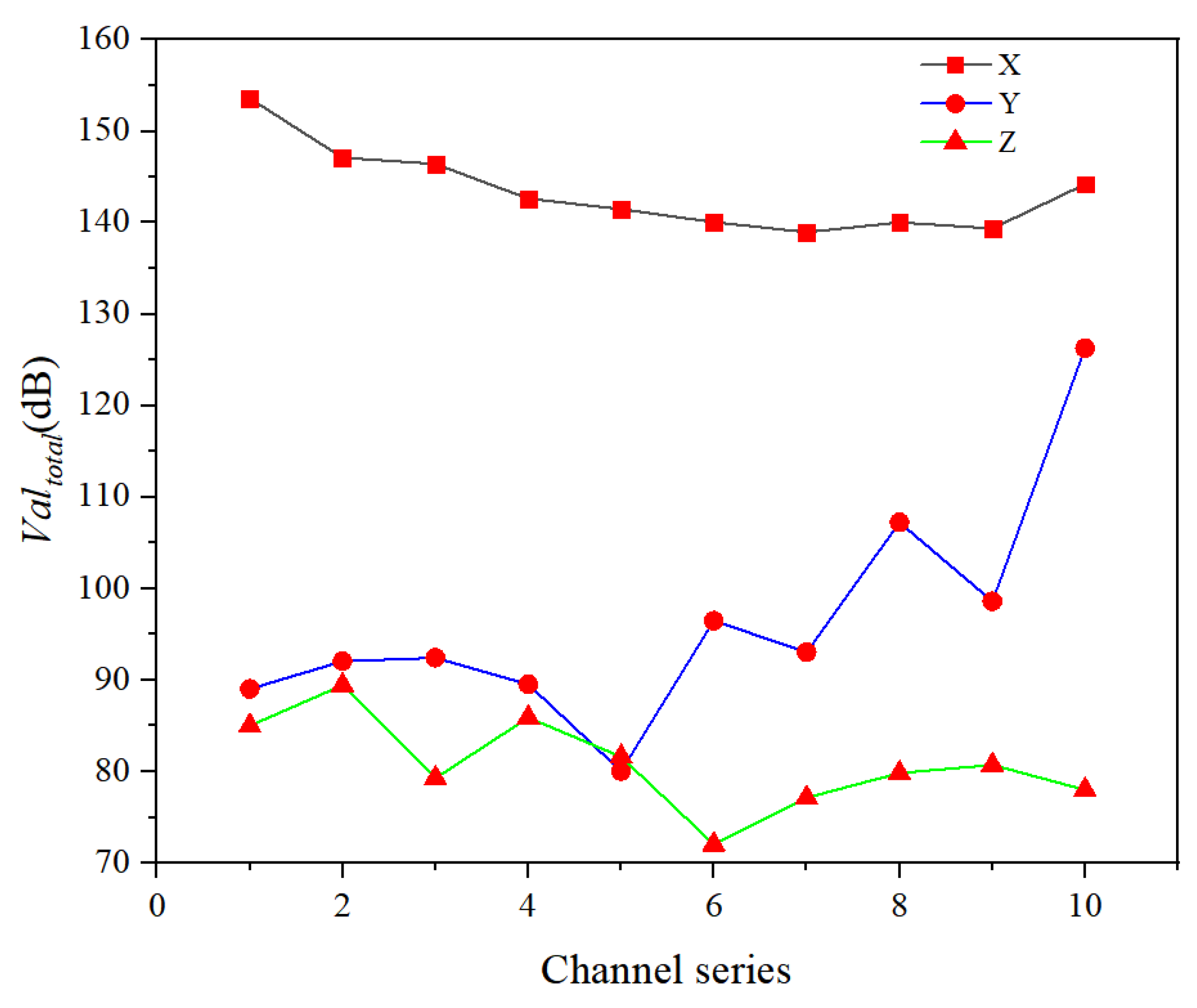
Figure 20 illustrates the overall vibration levels in each direction for the 10 stages of the spool flow path. It is evident that the total vibration levels in the X-direction exceed those in the Y- and Z-directions, with a minimal variation range. The maximum vibration level of 153.58 dB occurs in the first stage, while the minimum of 138.95 dB is observed in the seventh stage. The total vibration levels gradually decrease from the first stage, reaching their lowest point at the seventh stage, followed by a slight increase in stages eight, nine, and ten. In the Y-direction, the vibration levels exhibit a larger variation, with a minimum of 80.03 dB in the fifth stage and a maximum of 126.28 dB in the tenth stage. This range is significantly greater than those observed in the X- and Z-directions. In the Z-direction, the overall vibration levels are relatively low, with a maximum of 89.42 dB in the second stage and a minimum of 72.04 dB in the sixth stage. The fifth stage shows slightly higher total vibration levels compared to the Y-direction. In the first five stages, except for the third stage, the vibration levels are nearly identical to those in the Y-direction, after which they gradually increase. The differences in vibration intensity in the Z-direction, both at their peak and minimum, closely resemble those in the X-direction, with maximum and minimum differences of 17.4 dB and 14.6 dB, respectively.
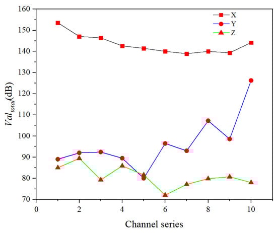
Figure 20.
Change curve of the total vibration level of each stage in different direction.
The figure reveals a non-uniform yet systematic distribution of total vibration levels across the spool flow channel stages in all three orthogonal directions. In the X-direction, the total vibration level exhibits a general decreasing trend with the increasing stage number, suggesting that fluid flow-induced spool vibration attenuates progressively along the channel. However, localized increases at the eighth to tenth stages may result from flow disturbances or geometric transitions at these locations. In the Y-direction, pronounced fluctuations in vibration levels reflect the complex hydrodynamic state within the flow path. The correlation between vibration trends and structural deformation patterns from the fifth stage onward implies potential flow channel shape modifications that subsequently alter flow characteristics and vibration behavior. Z-direction vibration levels remain comparatively low overall, indicating minimal fluid–structure interaction in this orientation. The notable exception occurs at the fifth stage, where Z-direction vibration slightly exceeds Y-direction levels. This anomaly may stem from transient flow phenomena such as vortex formation/dissipation or secondary flow development at this specific stage.
Based on the presented analysis, we conclude that the vibration acceleration spectrograms at the two measurement points show distinct characteristics in the three axes, which are closely linked to the flow dynamics within the channel. Therefore, these vibration characteristics must be thoroughly accounted for in the subsequent runner optimization design to minimize vibration-induced damage and improve the stability and reliability of the equipment. Vibration in the U-groove decreases progressively, except at the final stage, where the vibrations are most intense. In the three axes, the X-axis vibration has the greatest impact on deformation, the Z-axis shows the largest variation in vibration amplitude, and although the Y-axis vibration is partially mitigated due to wall support and fluid flow direction, it begins to increase from the fifth stage onward.
4. Conclusions
The FSI method was used to numerically simulate the vibration characteristics of the buck valve channel. A detailed analysis of the flow field within the valve is essential for understanding the vibration properties of sleeve control valves. Analyzing the flow dynamics inside the valve helps identify the sources of vibrations caused by fluid movement. This ultimately allows us to determine the vibration characteristics of the spool.
The flow characteristics reveal a multi-stage pressure reduction process within the flow passage, resulting in a gradual decrease in fluid pressure and a significant pressure drop. The outlet pressure at the final stage reaches the theoretically designed 1 MPa. The high-pressure flow velocity increases progressively through successive stages of pressure reduction, peaking at the sudden change in the outlet structure. Sharp declines, or even the complete cessation, of fluid velocity are observed at each stage of pressure reduction, causing turbulence due to variations in speed and changes in flow direction.
The structural analysis reveals that the primary and final vibration displacement of the flow channel valve core is most significant in the X-axis direction, followed by the Y-axis direction, and is least in the Z-axis direction, consistent with the flow field force. The lift coefficient CL of the flow field can reach up to 735, while the drag coefficient remains stable at −108. The drag coefficient on the Z-axis exhibits dramatic changes, with vortex shedding occurring in this direction, exerting a substantial influence. Vibration velocity and acceleration at the primary central measuring point are approximately three times greater than those at the final central measuring point, with significant initial vibration values and amplitudes. An analysis of the vibration acceleration spectrum indicates peak points corresponding to the first, third, and fourth mode frequencies. Maximum deformation suggests that vibration has a greater impact on the final stage compared to the primary stage. The total vibration level in the X-direction significantly exceeds that in other directions; meanwhile, the total vibration level in the Y-direction experiences larger amplitude changes with a maximum difference of 4.27 dB. The maximum and minimum differences in the Z-direction closely resemble those in the X-direction: 17.4 dB for the Z-direction and 14.6 dB for the X-direction.
Additionally, the pressure energy corresponding to a pressure difference of tens of megapascals is converted into heat, potentially causing thermal deformation of the part structure, which in turn affects the flow channel size. This effect is not considered in this study. Future studies should further investigate the specific effects of thermal deformation on flow channel size and its interaction with the dynamic characteristics of the flow field. Simultaneously, in-depth research on the energy loss mechanisms during high-pressure energy conversion is necessary to identify new methods for reducing energy loss and improving system efficiency. Furthermore, considering the impact of material non-linearity on spool vibration and flow field characteristics will provide more comprehensive guidance for optimal design.
In summary, the FSI method is used to numerically simulate and analyze the vibration characteristics of the valve spool step-down channel, leading to useful conclusions and insights. These conclusions not only enhance understanding of the spool’s vibration characteristics but also provide a theoretical foundation and technical support for optimizing spool design and improving performance.
Author Contributions
Writing—original draft preparation, H.X.; writing—review and editing, J.Z. and C.W.; project administration, X.L.; funding acquisition, H.J. All authors have read and agreed to the published version of the manuscript.
Funding
This work is supported by the National Key Research and Development Program of China (No. 2023YFC3010501), and The National Natural Science Foundation of China (No. 52176048).
Data Availability Statement
The original contributions presented in this study are included in the article. Further inquiries can be directed to the corresponding author.
Conflicts of Interest
The authors declare that they have no known competing financial interests or personal relationships that could have appeared to influence the work reported in this paper.
References
- Lin, Z.-H.; Hou, C.-W.; Zhang, L.; Guan, A.-Q.; Jin, Z.-J.; Qian, J.-Y. Fluid-structure interaction analysis on vibration characteristics of sleeve control valve. Ann. Nucl. Energy 2023, 181, 109579. [Google Scholar] [CrossRef]
- Jiang, Y.; Tao, J.; Zhu, L. Vibration fatigue analysis of liquid-filled pipelines considering fluid-structure interaction. In Advances in Engineering Materials, Structures and Systems: Innovations, Mechanics and Applications; CRC Press: Boca Raton, FL, USA, 2019; pp. 735–740. [Google Scholar]
- Zachwieja, J.; Peszyński, K. Determination of the Stress-Strain State for Industrial Pipeline Based on Its Vibration. In Proceedings of the 23rd International Conference Engineering Mechanics 2017, Svratka, Czech Republic, 15–18 May 2017. [Google Scholar]
- Yang, W.; Li, X.; Tao, Y.; Cen, K.; Wen, Y. Causal analysis of natural gas station pipelines vibration and reduction measures. J. Mech. Sci. Technol. 2022, 36, 4409–4418. [Google Scholar] [CrossRef]
- Bolin, C.; Engeda, A. Analysis of flow-induced instability in a redesigned steam control valve. Appl. Therm. Eng. 2015, 83, 40–47. [Google Scholar] [CrossRef]
- Lu, H.; Huang, K.; Wu, S. Vibration and stress analyses of positive displacement pump pipeline systems in oil transportation stations. J. Pipeline Syst. Eng. Pract. 2016, 7, 05015002. [Google Scholar]
- Zhang, L.; Wang, S.; Yin, G.; Guan, C. Fluid–structure interaction analysis of fluid pressure pulsation and structural vibration features in a vertical axial pump. Adv. Mech. Eng. 2019, 11, 1687814019828585. [Google Scholar] [CrossRef]
- Pei, J.; Meng, F.; Li, Y.; Yuan, S.; Chen, J. Fluid–structure coupling analysis of deformation and stress in impeller of an axial-flow pump with two-way passage. Adv. Mech. Eng. 2016, 8, 1687814016646266. [Google Scholar] [CrossRef]
- Oinonen, A. Water hammer and harmonic excitation response with fluid-structure interaction in elbow piping. J. Press. Vessel. Technol. 2022, 144, 031401. [Google Scholar] [CrossRef]
- Wang, W.; Zhang, L.; Ma, X.; Hu, Z.; Yan, Y. Experimental and numerical simulation study of pressure pulsations during hose pump operation. Processes 2021, 9, 1231. [Google Scholar] [CrossRef]
- Chen, L.; Zhang, H.; Huang, S.; Wang, B.; Zhang, C. Numerical Analysis of Flow-Induced Vibration of Heat Exchanger Tube Bundles Based on Fluid-Structure Coupling Dynamics. Model. Simul. Eng. 2022, 2022, 1467019. [Google Scholar]
- Wang, S.; Zhang, L.; Yin, G. Numerical investigation of the FSI characteristics in a tubular pump. Math. Probl. Eng. 2017, 2017, 7897614. [Google Scholar] [CrossRef]
- Chen, W.; Cao, Y.; Guo, X.; Ma, H.; Wen, B.; Wang, B. Semi-analytical dynamic modeling and fluid-structure interaction analysis of L-shaped pipeline. Thin-Walled Struct. 2024, 196, 111485. [Google Scholar] [CrossRef]
- Jin, H.; Xu, Z.; Zhang, J.; Liu, X.; Wang, C. Analysis of the pressure reduction mechanism in multi-stage counter-flow channels. Nucl. Eng. Des. 2024, 426, 113379. [Google Scholar] [CrossRef]
- Liu, F.; Wan, Z.; Cao, S.; Zhao, D.; Liu, G.; Zhang, K. Fluid-structure interaction analysis on flow field and vibration characteristics of gas proportional valve. Flow Meas. Instrum. 2025, 101, 102743. [Google Scholar] [CrossRef]
- Sun, X.; Li, X.; Zheng, Z.; Huang, D. Fluid–structure interaction analysis of a high-pressure regulating valve of a 600-MW ultra-supercritical steam turbine. Proc. Inst. Mech. Eng. Part A J. Power Energy 2015, 229, 270–279. [Google Scholar]
- Xie, Y.; Wang, Y.; Liu, Y.; Cao, F.; Pan, Y. Unsteady Analyses of a Control Valve due to Fluid-Structure Coupling. Math. Probl. Eng. 2013, 2013, 174731. [Google Scholar]
- Zong, C.; Li, Q.; Zheng, F.; Chen, D.; Li, X.; Song, X. Fluid-structure coupling analysis of a pressure vessel-pipe-safety valve system with experimental and numerical methods. Int. J. Press. Vessel. Pip. 2022, 199, 104707. [Google Scholar] [CrossRef]
- Ren, A.; Sun, H.; Wang, Y.; Zhang, M.; Sun, T. Deformation and vibration analysis of compressor rotor blades based on fluid-structure coupling. Eng. Fail. Anal. 2021, 122, 105216. [Google Scholar]
- Ye, W.; Liu, J.; Gan, L.; Wang, H.; Qin, L.; Zang, Q.; Bordas, S.P. Fluid-structure coupling analysis in liquid-filled containers using scaled boundary finite element method. Comput. Struct. 2024, 303, 107494. [Google Scholar] [CrossRef]


Disclaimer/Publisher’s Note: The statements, opinions and data contained in all publications are solely those of the individual author(s) and contributor(s) and not of MDPI and/or the editor(s). MDPI and/or the editor(s) disclaim responsibility for any injury to people or property resulting from any ideas, methods, instructions or products referred to in the content. |
© 2025 by the authors. Licensee MDPI, Basel, Switzerland. This article is an open access article distributed under the terms and conditions of the Creative Commons Attribution (CC BY) license (https://creativecommons.org/licenses/by/4.0/).