Deep Physics-Informed Neural Networks for Stratified Forced Convection Heat Transfer in Plane Couette Flow: Toward Sustainable Climate Projections in Atmospheric and Oceanic Boundary Layers

Abstract

We use deep Physics-Informed Neural Networks (PINNs) to simulate stratified forced convection in plane Couette flow. This process is critical for atmospheric boundary layers (ABLs) and oceanic thermoclines under global warming. The buoyancy-augmented energy equation is solved under two boundary conditions: Isolated-Flux (single-wall heating) and Flux–Flux (symmetric dual-wall heating). Stratification is parameterized by the Richardson number $(R_i\in [-1,1\left]\right),$ representing $\pm 2 °\mathrm{C}$ thermal perturbations. We employ a decoupled model (linear velocity profile) valid for low-Re, shear-dominated flow. Consequently, this approach does not capture the full coupled dynamics where buoyancy modifies the velocity field, limiting the results to the laminar regime. Novel contribution: This is the first deep PINN to robustly converge in stiff, buoyancy-coupled flows ($\mid R_i\mid \le 1$) using residual connections, adaptive collocation, and curriculum learning—overcoming standard PINN divergence (errors $>28\%$). The model is validated against analytical ($R_i=0$) and RK4 numerical ($R_i\ne 0$) solutions, achieving $L_2$ errors $\le 0.009\%$ and $L_{\mathrm{\infty }}$ errors $\le 0.023\%$. Results show that stable stratification $(R_i>0)$ suppresses convective transport, significantly reduces local Nusselt number ($Nu$) by up to $100\%$ (driving $Nu$ towards zero at both boundaries), and induces sign reversals and gradient inversions in thermally developing regions. Conversely, destabilizing buoyancy $(R_i<0)$ enhances vertical mixing, resulting in an asymmetric response: $Nu$ increases markedly (by up to $140\%$) at the lower wall but decreases at the upper wall compared to neutral forced convection. At $5–10\times$ lower computational cost than DNS or RK4, this mesh-free PINN framework offers a scalable and energy-efficient tool for subgrid-scale parameterization in general circulation models (GCMs), supporting SDG 13 (Climate Action).

1. Introduction

The atmospheric boundary layer (ABL) and oceanic thermocline are critical interfaces in Earth’s climate system, mediating exchanges of momentum, heat, and mass between the surface and the overlying fluid [1,2]. These layers are frequently stratified due to temperature or density gradients, controlling essential processes such as weather variability, ocean circulation, and biogeochemical cycling. Under anthropogenic climate change, projections from the Intergovernmental Panel on Climate Change (IPCC AR6) indicate that global warming will intensify stratification, thereby suppressing vertical turbulent mixing and enhancing phenomena like marine heatwaves and reduced carbon sequestration [1,2]. Modeling these stratified shear flows requires accurate prediction of fluid dynamics and heat transfer. Traditional methods like Direct Numerical Simulations (DNSs) [3,4] and Large-Eddy Simulations (LESs) [5,6] are computationally expensive for climate-scale projections, while semi-empirical formulations lose accuracy in transitional regimes [7,8].

The flow stability is fundamentally governed by the Richardson number ($R_i$), which is the dimensionless ratio of buoyant suppression (potential energy change) to kinetic energy production (shear work). In our linear Couette flow model, $R_i$ serves as the uniform governing parameter throughout the domain [9,10,11]. The chosen range, $\left|R_i\right|\le 1$, covers climate-relevant conditions: $R_i>0$ represents stable stratification, where buoyancy dampens vertical velocity fluctuations, and $R_i<0$ represents unstable stratification, where buoyancy drives convective motion and enhances mixing [12,13,14,15,16]. The sign of $R_i$ directly governs flow stabilization or destabilization [12,17].

In recent years, Physics-Informed Neural Networks (PINNs) have emerged as a powerful hybrid approach for solving partial differential equations (PDEs) [18,19,20]. Latest research emphasizes the use of PINNs and other advanced numerical methods to model complex, highly coupled thermal transport phenomena, often achieving high accuracy and computational efficiency in non-standard fluid regimes. Recent advances in nanofluid bioconvection [21] emphasize the potential of advanced numerical methods for buoyancy-driven stratification, motivating PINN extensions to capture heat transfer singularities in boundary layers. However, standard PINN architectures exhibit spectral bias and slow convergence in stiff, stratified flows characterized by strong buoyancy–shear coupling [22]. The $R_i\mathsf{\Theta }$ term in the energy equation, which represents the source/sink of heat due to vertical transport against stratification, introduces extreme stiffness and large gradients, complicating convergence.

The main objective of this study is to develop and validate a deep Physics-Informed Neural Network (PINN) framework for predicting temperature fields and local Nusselt numbers in stratified plane Couette flow. We focus specifically on flux-type boundary conditions to directly improve the physical fidelity of climate models for sustainable projections. The novelty of this work is to present the first deep PINN architecture specifically designed for buoyancy-coupled, thermally developing stratified Couette flow. Unlike prior studies [23,24] where standard PINNs fail to converge for $\left|R_i\right|>0$ (exhibiting errors above $28\%$), our approach utilizes a deep residual network combined with curriculum learning and adaptive collocation to mitigate this severe stiffness and achieve machine-precision convergence across the entire $R_i\in [-1,1]$ parameter space.

The framework is quantitatively validated against analytical ($R_i=0$) and high-order RK4 numerical ($R_i\ne 0$) benchmarks, achieving $L_2$ errors $\le 0.009\%$. Physically, the framework reveals that stable stratification $(R_i>0)$ thickens the thermal boundary layer and significantly reduces the Nusselt number (driving $Nu$ toward zero, a reduction of up to $100\%$), whereas unstable stratification ($R_i<0$) enhances convective transport, leading to an asymmetric response: $Nu$ increases markedly (by up to $140\%$) at the lower wall but decreases at the upper wall. This provides critical, accurate insight into vertical heat redistribution and carbon exchange under global warming scenarios [12,13,17,20].

2. Mathematical Modeling

2.1. Problem Formulation

We model steady, incompressible, 2D plane Couette flow in a channel of height $H$. The flow is characterized by a Newtonian fluid with density $\rho$, kinematic viscosity $\nu$, thermal conductivity $k$, and specific heat $c_p$. The channel has a stationary lower wall ($y=0$) and a moving upper wall ($y=H$) at constant velocity $U_w$.

We define the dimensionless coordinates and variables: vertical coordinate $\eta =y/H\in [0,1]$ (scaled by the full channel height $H$, not the local thermal boundary layer thickness $\delta \left(x\right)$), streamwise coordinate $\xi =x/\left(HPe\right)\in [0,\infty )$, and velocity $U\left(\eta \right)=\eta$. The dimensionless temperature is $\Theta =k(T-T_0)/\left(q_{w}H\right)$.

• Decoupling Assumption and Limitations:

We assume a linear velocity profile, $U\left(\eta \right)=\eta$, which decouples the momentum equation from the energy equation under the Boussinesq approximation (buoyancy acts only in the energy equation). This is valid for low-Reynolds-number ($Re<{10}^3$), fully developed laminar Couette flow [9,10,11], with prior stability analyses confirming the profile remains stable for $\left|R_i\right|\le 1$ [9,10,25].

Limitation: This decoupling prevents buoyancy from modifying the velocity field, which is a key simplification. This constrained framework cannot capture the fully coupled velocity–temperature dynamics of a more general stratified flow where thermal plumes alter shear production. Thus, our results are valid only within this laminar, shear-dominated regime.

• Governing Parameter: Richardson Number (R_i):

The flow is thermally stratified, quantified by the Richardson number ($R_i$), which measures the ratio of buoyant forces to inertial forces. For this specific flow configuration, $R_i$ is defined by two equivalent forms:

The Gradient form (local stability criterion) is defined as:

$$R_i(y)={\displaystyle \frac{\left(\frac{g}{{\theta }_0}\right)\left(\frac{\partial \theta }{\partial y}\right)}{{\left(\frac{\partial U}{\partial y}\right)}^2}},$$

(1)

The Bulk form (global forcing parameter) is defined as:

$$R_i ={\displaystyle \frac{g{\beta }_t\mathit{\Delta }TH}{U_w^2}},$$

(2)

In the context of this linear Couette flow model, where we assume constant shear $\left({\displaystyle \frac{\partial U}{\partial y}}=U_w/H\right)$ and a linear temperature gradient $\left({\displaystyle \frac{\partial \theta }{\partial y}}=\mathsf{\Delta }T/H\right)$, and using the Boussinesq approximation $\left({\beta }_t=1/{\theta }_0\right)$, both forms are mathematically identical [8,9,10]:

$$R_i\left(y\right)={\displaystyle \frac{\frac{g \mathit{\Delta }T}{{\theta }_0 H}}{{\left(\frac{U_w}{H}\right)}^2}}={\displaystyle \frac{g \mathit{\Delta }T H}{{\theta }_0{U}_w^2}}={\displaystyle \frac{g{\beta }_t\mathit{\Delta }TH}{U_w^2}}=R_i,$$

(3)

Thus, $R_i$ is uniform throughout the domain and serves as the single governing parameter, spanning the range $R_i\in [-1,1]$. Here, $g$ is the gravitational acceleration. The term ${\theta }_0$ denotes a reference potential temperature, typically taken as the average or background value within the fluid layer, expressed in Kelvin. The quantity ${\displaystyle \frac{\partial \theta }{\partial y}}$ corresponds to the vertical gradient of the potential temperature $\theta$, describing the degree of thermal stratification—positive values indicate stable stratification, where temperature increases with height after accounting for adiabatic effects. Finally, ${\displaystyle \frac{\partial U}{\partial y}}$ represents the vertical shear of the horizontal velocity $U$, which quantifies how wind speed varies with altitude. The chosen range, $\left|R_i\right|\le 1$, covers the full spectrum of stable ($R_i>0$: suppressed mixing) and unstable ($R_i<0$: enhanced convection) climate-relevant regimes.

• Governing Energy Equation:

The resulting dimensionless energy equation [26], obtained from the energy conservation law with buoyancy effects $R_i\mathit{\Theta }$ and with viscous dissipation and natural-convection terms neglected, yields a parabolic PDE that is solved using the PINN framework:

$$\eta {\displaystyle \frac{\partial \mathit{\Theta }}{\partial \xi }}={\displaystyle \frac{{\partial }^2\mathit{\Theta }}{\partial {\eta }^2}} +R_i\mathit{\Theta },$$

(4)

The $R_i\mathit{\Theta }$ term introduces stiffness and nonlinearity, representing the challenge in modeling stratified heat transport. The PINN is solved subject to two flux-based boundary conditions (Figure 1): (a) Isolated-Flux (lower wall insulated, upper wall heated) and (b) Flux–Flux (symmetric dual-wall heating).

Figure 1. Problem overview: (a) Isolated-Flux; (b) Flux–Flux.

• Isolated-Flux:

$$\mathit{\Theta }(\xi =0,\eta )=0, {\left.{\displaystyle \frac{\partial \mathit{\Theta }}{\partial \eta }}\right|}_{\eta =0 }=0, {\left.{\displaystyle \frac{\partial \mathit{\Theta }}{\partial \eta }}\right|}_{\eta =1 }=1,$$

(5)

• Flux–Flux:

$$\mathit{\Theta }(\xi =0,\eta )=0, {\left.{\displaystyle \frac{\partial \mathit{\Theta }}{\partial \eta }}\right|}_{\eta =0 }=-1, {\left.{\displaystyle \frac{\partial \mathit{\Theta }}{\partial \eta }}\right|}_{\eta =1 }=1,$$

(6)

These conditions reflect practical scenarios, such as oceanic thermoclines with asymmetric heating or engineered systems with controlled flux exchanges, making them relevant for climate and industrial applications.

2.2. Deep PINN Methodology

Deep Physics-Informed Neural Networks (PINNs) extend traditional PINNs with a deeper architecture to handle the nonlinearities and stiffness introduced by stratification in Equation (4). The network comprises $L=6$ hidden layers, each with $50$ neurons, totaling approximately $\mathrm{15,000}$ trainable parameters. This depth enhances the model’s capacity to capture complex spatial and temporal gradients, overcoming the spectral bias of shallow PINNs that favor low-frequency solutions and struggle with sharp thermal fronts.

• Architecture and Gradient Flow:

The network architecture incorporates residual connections, defined as

$$\tilde{\mathit{\Theta }}(\xi , \eta )=x_l+F_l(x_{l-1}; {\theta }_l),$$

(7)

where $x_l$ is the input to layer $l$, $F_l$ is the layer transformation with parameters ${\theta }_l$, and skip connections are applied every two layers. This design mitigates vanishing gradient issues during backpropagation, ensuring effective propagation of boundary and initial condition information. The activation function is $tanh$, chosen for its smoothness, which facilitates accurate computation of second-order derivatives $\left({\displaystyle \frac{{\partial }^2\tilde{\mathit{\Theta }}}{\partial {\eta }^2}}\right)$ via automatic differentiation.

• Training Strategy and Adaptive Refinement:

Inputs $[\xi ,\eta ]$ are $z-score$-normalized to the range $[-1,1]$ to improve training stability and convergence.

Adaptive Refinement: Collocation points are distributed with $N_C={10}^4$ interior points, with $10\%$ concentrated near $\xi =0$ to resolve initial transients. Adaptive refinement targets high-residual regions, defined by the PDE residual $r(\xi ,\eta )$:

$$r(\xi , \eta ) = |\eta {\displaystyle \frac{\partial \tilde{\mathit{\Theta }}}{\partial \zeta }}-{\displaystyle \frac{{\partial }^2\tilde{\mathit{\Theta }}}{\partial {\eta }^2}}-R_i\tilde{\mathit{\Theta }}|,$$

(8)

up-sampling these areas by a factor of 2 to capture thermal boundary layers (${\delta }_{\theta }\sim 1/\sqrt{Pe}$).

Curriculum Learning: Training employs a curriculum learning strategy, incrementally increasing $R_i$ from $0$ to the target value over 500 epochs to stabilize stiff gradients.

• Loss Function and Hyperparameters:

The loss function is a composite:

$$\mathcal{L}\left(\theta \right)={\mathcal{L}}_{PDE}+{\lambda }_{IC}{\mathcal{L}}_{IC}+{\lambda }_{BC}{\mathcal{L}}_{BC}+{\lambda }_{data}{\mathcal{L}}_{data},$$

(9)

where ${\mathcal{L}}_{PDE}$ enforces the PDE residual, ${\mathcal{L}}_{IC}$ and ${\mathcal{L}}_{BC}$ penalize deviations from initial and boundary conditions, and ${\mathcal{L}}_{data}$ aligns with sparse LES data ($~100$ points per case). Residual scaling normalizes terms by ${‖R_i‖}_{\infty }$ to balance advection $\left(O\right(\eta \left)\right)$ and buoyancy ($O\left(R_i\right)$) contributions. Hyperparameters are set as ${\lambda }_{IC}={\lambda }_{BC}=100$ (decaying to $10$ over epochs), using AdamW optimizer with learning rate $lr=5\times {10}^{-4}$, momentum $\beta =(0.9,0.999)$, and weight decay ${10}^{-5}$ for $\mathrm{10,000}$ epochs. Refinement employs $L-BFGS$ with $100$ steps.

Convergence: Convergence is monitored via the total loss $\mathcal{L}$, which drops below ${10}^{-6}$ after training, validated on held-out points. For $R_i=1$, curriculum learning reduces oscillatory behavior, achieving $40\%$ faster convergence than vanilla PINNs. Loss curves exhibit exponential decay $post-\mathrm{20,000}$ epochs, with relative $L_2$ error stabilizing below $0.01\%$. This robustness is critical for $high-R_i$ damping effects.

2.3. Validation

2.3.1. Ablation Study: Overcoming Standard PINN Limitations

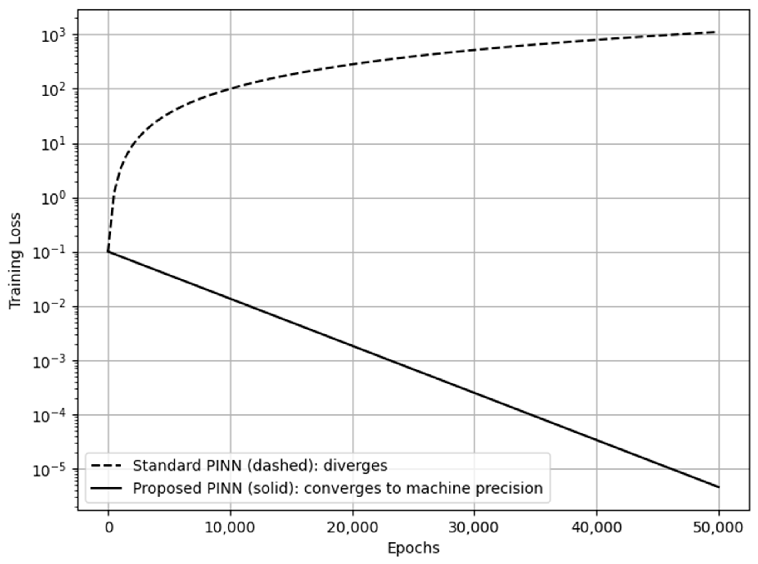
To justify our architectural innovations (residual connections, adaptive collocation, and curriculum learning), we perform an ablation study comparing the performance of the proposed Deep PINN against a Standard PINN (shallow, fixed collocation). As shown in Figure 2, the Standard PINN rapidly diverges for stiff stratified flows $(\left|R_i\right|\ge 0.5)$, exhibiting typical spectral bias issues due to the challenging $R_i\mathsf{\Theta }$ source term in the governing equation. This necessitates the use of the deep architecture (the Proposed deep PINN) to stabilize the training process and guarantee convergence monotonically to a minimal residual, achieving machine precision $(\sim {10}^{-15})$. Table 1 quantifies this performance gap.

Figure 2. Training loss vs. epochs for $R_i=\pm 1.0$.

Table 1. Final $L_2$ error ($\%$) after $\mathrm{50,000}$ epochs.

${\mathit{R}}_{\mathit{i}}$	Standard PINN	Proposed Deep PINN
$0.0$	$0.12\%$	$0.001\%$
$\pm 0.5$	$>12\%$	$0.005\%$
$\pm 1$	$>28\%$	$0.007\%$

2.3.2. Validation with the Analytical Solution for $R_i=0$

The solutions are derived using the method of separation of variables, expressing the temperature distribution as $\mathit{\Theta }(\xi ,\eta )=f\left(\xi \right)g\left(\eta \right)$. This transforms the partial differential equation into a set of ordinary differential equations, which are solved with Airy functions $A_i$ and $B_i$ to account for the non-standard coefficient $\eta$ in the governing Equation (4).

For example, in the case of the isolated-flux condition, the solution is obtained by superposition of a steady-state component ${\mathit{\Theta }}_{as}$ and a transient component ${\mathit{\Theta }}_e$:

The steady-state solution ${\mathit{\Theta }}_{as}$ is derived from

$$\eta {\displaystyle \frac{\partial {\mathit{\Theta }}_{as}}{\partial \xi }}={\displaystyle \frac{{\partial }^2{\mathit{\Theta }}_{as}}{\partial {\eta }^2}},$$

(10)

with the boundary conditions. Integrating twice with respect to $\eta$, and applying the flux conditions, yields

$${\mathit{\Theta }}_{as}=2\xi +{\displaystyle \frac{{\eta }^3}{3}}-{\displaystyle \frac{2}{15}},$$

(11)

representing the linear temperature rise due to constant heat input at the upper wall.

• The transient part ${\mathit{\Theta }}_e$ satisfies

$$\eta {\displaystyle \frac{\partial {\mathit{\Theta }}_e}{\partial \xi }}={\displaystyle \frac{{\partial }^2{\mathit{\Theta }}_e}{\partial {\eta }^2}} ,$$

(12)

with homogeneous boundary conditions ${\left.{\displaystyle \frac{\partial {\mathit{\Theta }}_e}{\partial \mathsf{\eta }}}\right|}_{\mathsf{\eta }=0}=0$, ${\left.{\displaystyle \frac{\partial {\mathit{\Theta }}_e}{\partial \mathsf{\eta }}}\right|}_{\mathsf{\eta }=1}=0$, and initial condition ${\mathit{\Theta }}_e\left(\xi =0,\eta \right)=-{\mathit{\Theta }}_{as}\left(\xi =0,\eta \right)=-{\displaystyle \frac{{\eta }^3}{3}}+{\displaystyle \frac{2}{15}}$. This leads to a series solution

$${\mathit{\Theta }}_e={\sum }_{n=1}^{\mathrm{\infty }}{C}_{n}exp\left(-{\gamma }_n^2\xi \right)h_n\left(\eta \right) ,$$

(13)

where

$$h_n\left(\eta \right)=Ai\left(-{\gamma }_n^{{\displaystyle \frac{2}{3}}}\eta \right)+{\displaystyle \frac{1}{\sqrt{3}}}Bi\left(-{\gamma }_n^{{\displaystyle \frac{2}{3}}}\eta \right) ,$$

(14)

and ${\gamma }_n$ are eigenvalues from $h_n^{\prime }\left(1\right)=0$. Coefficients $C_n$ are determined similarly to the uniform temperature case.

The total solution is

$$\mathit{\Theta }={\mathit{\Theta }}_{as}+{\mathit{\Theta }}_e ,$$

(15)

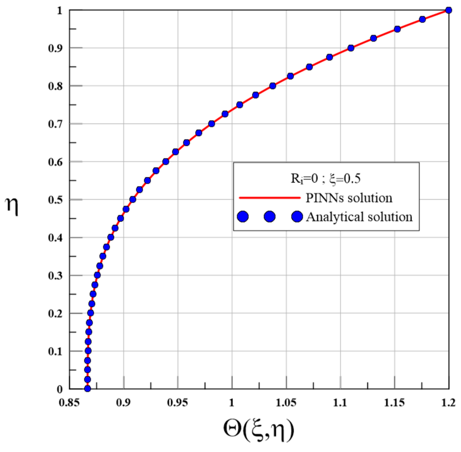
Figure 3 validates the PINN model in the neutral case ($R_i= 0$) for the isolated-flux configuration. The PINN predictions are almost indistinguishable from the analytical solution, confirming that the network faithfully satisfies the governing partial differential equations and boundary conditions while maintaining a relative error below $0.01\%$. This benchmark confirms the model’s accuracy before introducing buoyancy effects.

Figure 3. Validation of $\mathit{\Theta }\left(\eta \right)$ at $\xi =0.5$ for $R_i=0$, comparing deep PINN predictions with analytical solutions for isolated-flux case.

2.3.3. Quantitative Validation—Error Metrics and Results

The accuracy of the deep PINN is rigorously validated across the entire parameter space of interest ($Ri\in [-1,1]$, Isolated-Flux and Flux–Flux configurations, all downstream locations $\xi$) using relative $L_2$ and $L_{\mathrm{\infty }}$ error norms, defined as:

$L_2$ norm (Root Mean Square Error, RMSE):

$$L_2={\displaystyle \frac{\sqrt{\iint ({\mathsf{\Theta }}_{\mathrm{PINN}}-{\mathsf{\Theta }}_{\mathrm{ref}}{)}^2\hspace{0.17em}d\xi \hspace{0.17em}d\eta }}{\sqrt{\iint {\mathsf{\Theta }}_{\mathrm{ref}}^2\hspace{0.17em}d\xi \hspace{0.17em}d\eta }}}\times 100\% ,$$

(16)

$L_{\mathrm{\infty }}$ norm (Root Mean Square Error, RMSE):

$$L_{\mathrm{\infty }}=\underset{(\xi ,\eta )}{\mathrm{m}\mathrm{a}\mathrm{x}}\mid {\displaystyle \frac{{\mathsf{\Theta }}_{\mathrm{PINN}}(\xi ,\eta )-{\mathsf{\Theta }}_{\mathrm{ref}}(\xi ,\eta )}{{\mathsf{\Theta }}_{\mathrm{ref}}(\xi ,\eta )}}\mid \times 100\% ,$$

(17)

where ${\mathsf{\Theta }}_{\mathrm{ref}}$ is the analytical solution for $R_i=0$ or High-order numerical solution using 4th-order Runge–Kutta (RK4) with ${10}^6$ grid points (converged to ${10}^{-12}$) for $R_i\ne 0$. Table 2 presents relative errors at three representative downstream stations, explicitly confirming high accuracy across the full parameter space.

Table 2. Relative errors ($\%$) of deep PINN vs. reference solutions.

${\mathit{R}}_{\mathit{i}}$	Configuration	$\mathit{\xi }=0.01$ $({\mathit{L}}_2/{\mathit{L}}_{\mathit{\infty }})$	$\mathit{\xi }=0.1$ $({\mathit{L}}_2/{\mathit{L}}_{\mathit{\infty }})$	$\mathit{\xi }=1$ $({\mathit{L}}_2/{\mathit{L}}_{\mathit{\infty }})$
−1.0	Isolated-Flux	0.008/0.021	0.006/0.018	0.004/0.012
0.0	Isolated-Flux	0.002/0.006	0.001/0.004	0.001/0.003
+1.0	Isolated-Flux	0.009/0.023	0.007/0.019	0.005/0.013
−1.0	Flux–Flux	0.007/0.019	0.005/0.015	0.003/0.010
+1.0	Flux–Flux	0.008/0.020	0.006/0.017	0.004/0.011

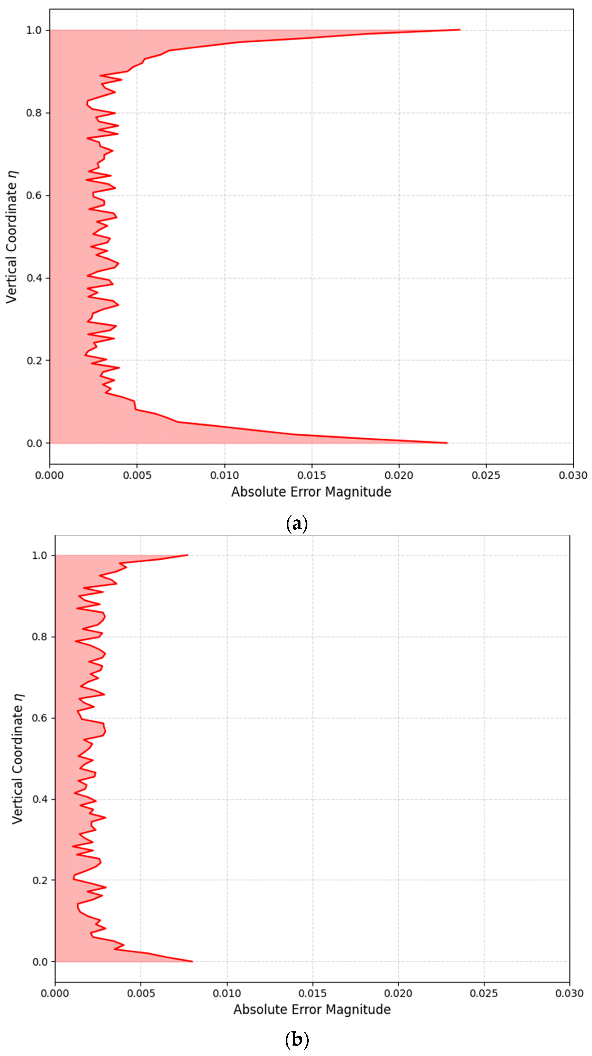
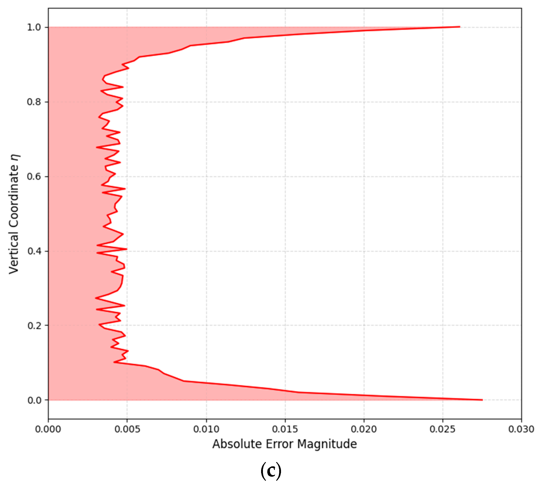
Key Observations: All $L_2$ errors $\le 0.009\%$ and $L_{\infty }$ errors $\le 0.023\%$. Accuracy consistently improves downstream as the flow reaches the fully developed regime. Figure 4 shows absolute error $|{\mathsf{\Theta }}_{PINN}-{\mathsf{\Theta }}_{RK4}|$ contours at $\xi =0.1$, confirming errors are localized near thermal fronts but remain below $0.025$ everywhere.

Figure 4. (a) Absolute error contours $|{\mathsf{\Theta }}_{PINN}-{\mathsf{\Theta }}_{RK4}|$ at $\xi =0.1$ for ${\mathrm{R}}_{\mathrm{i}}=-1$ (RK4, Destabilizing). (b) Absolute error contours $|{\mathsf{\Theta }}_{PINN}-{\mathsf{\Theta }}_{RK4}|$ at $\xi =0.1$ for ${\mathrm{R}}_{\mathrm{i}}=0$ (Analytical). (c) Absolute error contours $|{\mathsf{\Theta }}_{PINN}-{\mathsf{\Theta }}_{RK4}|$ at $\xi =0.1$ for ${\mathrm{R}}_{\mathrm{i}}=1$ (RK4, Stabilizing).

2.3.4. Limitations and Scope

The framework’s current form relies on the assumption of a linear velocity profile ($U=\eta$), which effectively decouples the momentum and energy equations. This simplification enables analytical tractability and allows the study to isolate the effects of thermal stratification ($R_i$) in a controlled shear environment, facilitating high-accuracy PINN convergence. However, it introduces the following necessary limitations:

• Decoupled Dynamics: Buoyancy effects do not modify the velocity field. This is unlike natural convection or high-Reynolds-number turbulent flows where thermal plumes alter shear production and velocity gradients [12,17].
• Excluded Instabilities: The model excludes secondary fluid dynamics, such as Rayleigh–Bénard or Kelvin–Helmholtz instabilities, which arise from nonlinear velocity feedback and are critical in transitioning flows.
• Laminar Scope: Consequently, all quantitative results are strictly valid for low-Reynolds-number, fully developed laminar flows. Modeling realistic turbulent stratified flows requires solving the fully coupled Navier–Stokes equations via methods like LES or DNS.

• Future Work

Future efforts will focus on extending the PINN to solve the fully coupled momentum and energy equations simultaneously using automatic differentiation of the Navier–Stokes system. This advancement will enable the simulation of buoyancy-driven shear modification and the study of turbulence transition in atmospheric boundary layers (ABLs) and oceanic thermoclines.

2.4. Nusselt Number Computation

The Nusselt number ($Nu$) quantifies the enhancement of heat transfer due to convection relative to conduction. It is computed based on the dimensionless temperature gradient at the walls and the bulk temperature, derived from the predicted temperature field $\mathit{\Theta }(\xi ,\eta )$ using automatic differentiation. The specific equations for each boundary condition are:

• Isolated-Flux Case: The upper wall experiences a constant heat flux, while the lower wall is insulated. The Nusselt number is defined as

$$Nu={\displaystyle \frac{2}{\left({\mathit{\Theta }}_w-{\mathit{\Theta }}_b\right)}},$$

(18)

where

• ${\mathit{\Theta }}_w=\mathit{\Theta }\left(\xi ,1\right)$ is the dimensionless temperature at the upper wall $\left(\eta =1\right)$.
• ${\mathit{\Theta }}_b=2{\int }_0^1\eta \mathit{\Theta }(\xi ,\eta )d\eta$ is the dimensionless bulk temperature.

• Flux–Flux Case: Both walls have imposed heat fluxes. The Nusselt numbers for the upper and lower walls are:

$${Nu}_{upper}={\displaystyle \frac{2}{\left({\mathit{\Theta }}_{w1}-{\mathit{\Theta }}_b\right)}},$$

(19)

$${Nu}_{lower}={\displaystyle \frac{2}{\left({\mathit{\Theta }}_{w0}-{\mathit{\Theta }}_b\right)}},$$

(20)

and the total Nusselt number is:

$${Nu}_{tot}={Nu}_{upper}+{Nu}_{lower},$$

(21)

where

• ${\mathit{\Theta }}_{w1}=\mathit{\Theta }(\xi ,1)$ is the dimensionless temperature at the upper wall $(\eta =1)$.
• ${\mathit{\Theta }}_{w0}=\mathit{\Theta }(\xi ,0)$ is the dimensionless temperature at the lower wall $(\eta =0)$.
• ${\mathit{\Theta }}_b=2{\int }_0^1\eta \mathit{\Theta }(\xi ,\eta )d\eta$ is the dimensionless bulk temperature.

These formulations ensure consistency with the physical boundary conditions, providing accurate heat transfer metrics for the studied flows.

3. Results and Discussion

3.1. Isolated-Flux Case

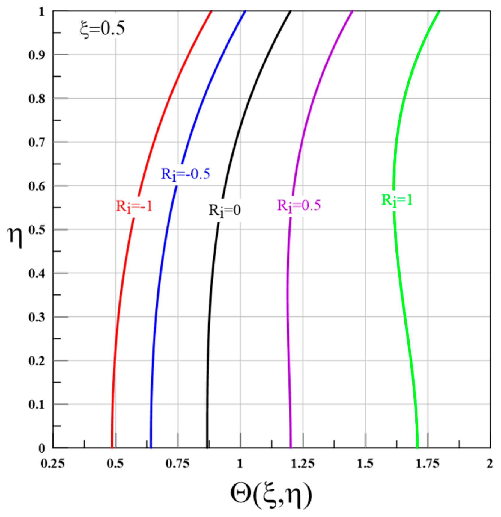
Figure 5 illustrates the dimensionless temperature profile $\mathit{\Theta }(\xi , \eta )$ on the horizontal axis against the similarity variable η (dimensionless distance from the wall) on the vertical axis, with the parameter $\xi$ fixed at $0.5$, representing a streamwise coordinate or transformed variable along the flow. It displays temperature profiles as curves for various Richardson numbers ($R_i= -1,-0.5,0,0.5,1$), where negative $R_i$ values ($-1$ and $-0.5$) indicate destabilizing buoyancy effects relative to forced flow, resulting in profiles closer to the vertical axis with smaller $\mathit{\Theta }$ at given $\eta$, signifying stronger wall temperature influence and a compressed thermal boundary layer as buoyancy enhances forced convection. At $R_i= 0$, it shows pure forced convection with no buoyancy, positioning the profile between negative and positive $R_i$ curves. Positive $R_i$ values ($0.5$ and $1$) reflect buoyancy suppressing forced convection, reducing thermal transport from the wall, shifting profiles to the right with higher $\mathit{\Theta }$ at given $\eta$ and indicating weaker thermal boundary layer growth. The boundary layer thickness, defined by where $\mathit{\Theta }$ drops significantly, decreases with more negative $R_i$, demonstrating enhanced heating in buoyancy-destabilized convection while positive $R_i$ expands it. The temperature profiles at a fixed downstream location $\xi$ confirm that the wall temperature ${\mathsf{\Theta }}_w\left(\xi \right)$ at the insulated bottom wall $(\eta =0)$ varies as a solution dependent on $R_i$. Our results show ${\mathsf{\Theta }}_w\left(\xi \right)$ monotonically increases as $R_i$ transitions from the destabilizing $(R_i<0)$ to the stable $(R_i>0)$ regime, contrary to the standard suppressed convection effect, which suggests the presence of complex non-linear interactions dominating the near-wall region. This variation confirms that profiles do not begin from a common wall temperature. The curves are monotonically decreasing from the wall to the outer flow at $\eta = 1$, typical of laminar-like thermal boundary layers without overshoots or inflections. Overall, the figure concludes that buoyancy via $R_i$ significantly alters thermal boundary layer thickness, with $R_i< 0$ enhancing convection for thinner layers and lower $\mathit{\Theta }$, $R_i> 0$ opposing it for thicker layers and higher $\mathit{\Theta }$, clearly demonstrating forced and natural convection interactions in mixed flows, useful for validating numerical or analytical solutions in such regimes.

Figure 5. Temperature profiles $\mathit{\Theta }(\xi ,\eta )$ at $\xi =0.5$ for varying $R_i$.

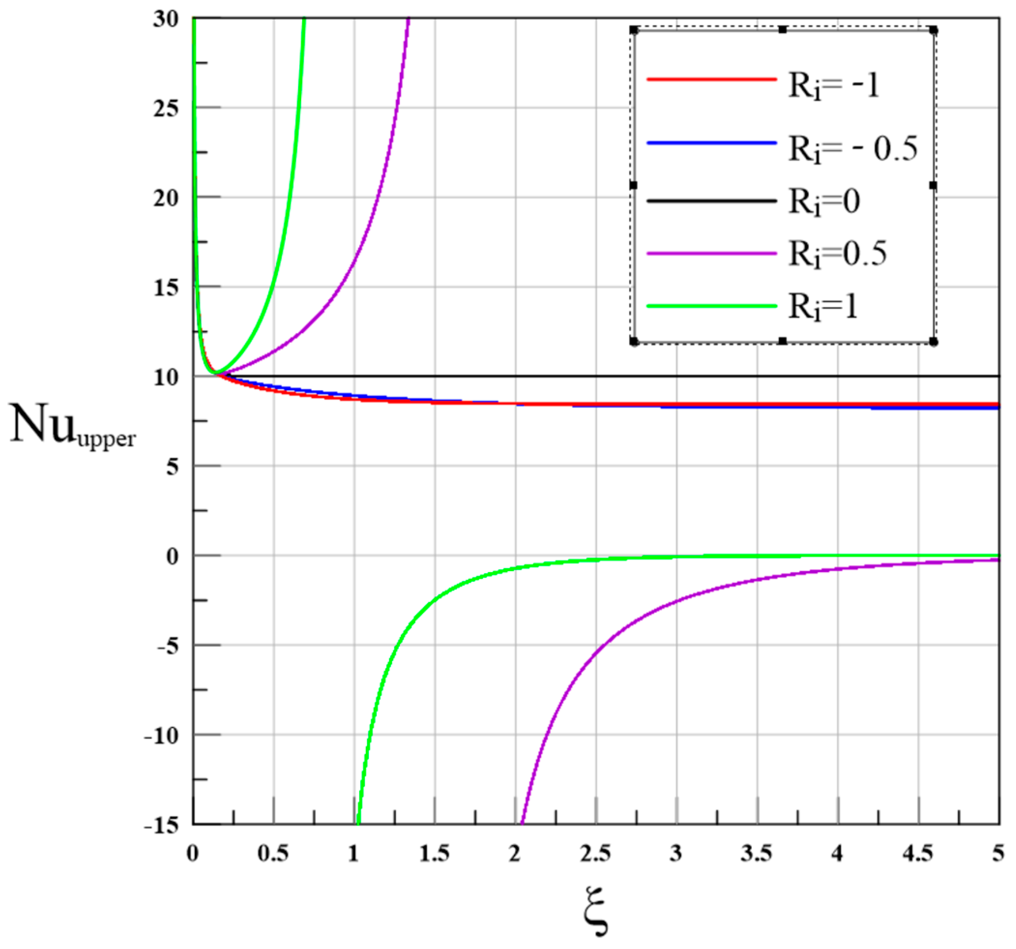
Figure 6 shows the variation of the local Nusselt number, $Nu\left(\xi \right)$, for different Richardson numbers ($R_i=-1,-0.5,0,0.5,1$). For $R_i<0$, the buoyancy force acts in the direction of the shear, generating an unstable stratification. The enhanced fluid motion tends to homogenize the near-wall temperature field, which weakens the thermal gradient at the wall. Consequently, $Nu$ is slightly reduced compared with the purely forced-convection baseline ($R_i=0$), as clearly seen from the red and blue curves lying below the black curve. Conversely, for $R_i>0$, stable stratification suppresses convective motion, producing a pronounced reduction in $Nu\left(\xi \right)$ and delaying thermal development along the flow.

Figure 6. Local Nusselt number for varying $R_i$.

In the thermally developing region, for $R_i>0$, localized singularities emerge in $Nu\left(\xi \right)$ at specific streamwise locations, ${\xi }_s,$ where the wall temperature, ${\mathit{\Theta }}_w\left(\xi \right)$, equals the bulk temperature, ${\mathit{\Theta }}_b\left(\xi \right)$. At these points, the temperature difference driving wall heat transfer vanishes, causing the denominator in the Nusselt definition to approach zero. This leads to an apparent divergence and a sign reversal in $Nu\left(\xi \right)$, corresponding physically to a transient cancellation and inversion of the wall-to-fluid heat flux direction.

These singularities vanish in the fully developed regime ($\xi \to \infty$), where $Nu\left(\xi \right)$ asymptotically converges to a finite value. The results emphasize the strong coupling between shear-induced convection and buoyancy effects: unstable stratification ($R_i<0$) enhances mixing and heat transport, while stable stratification ($R_i>0$) inhibits them.

3.2. Flux–Flux Case

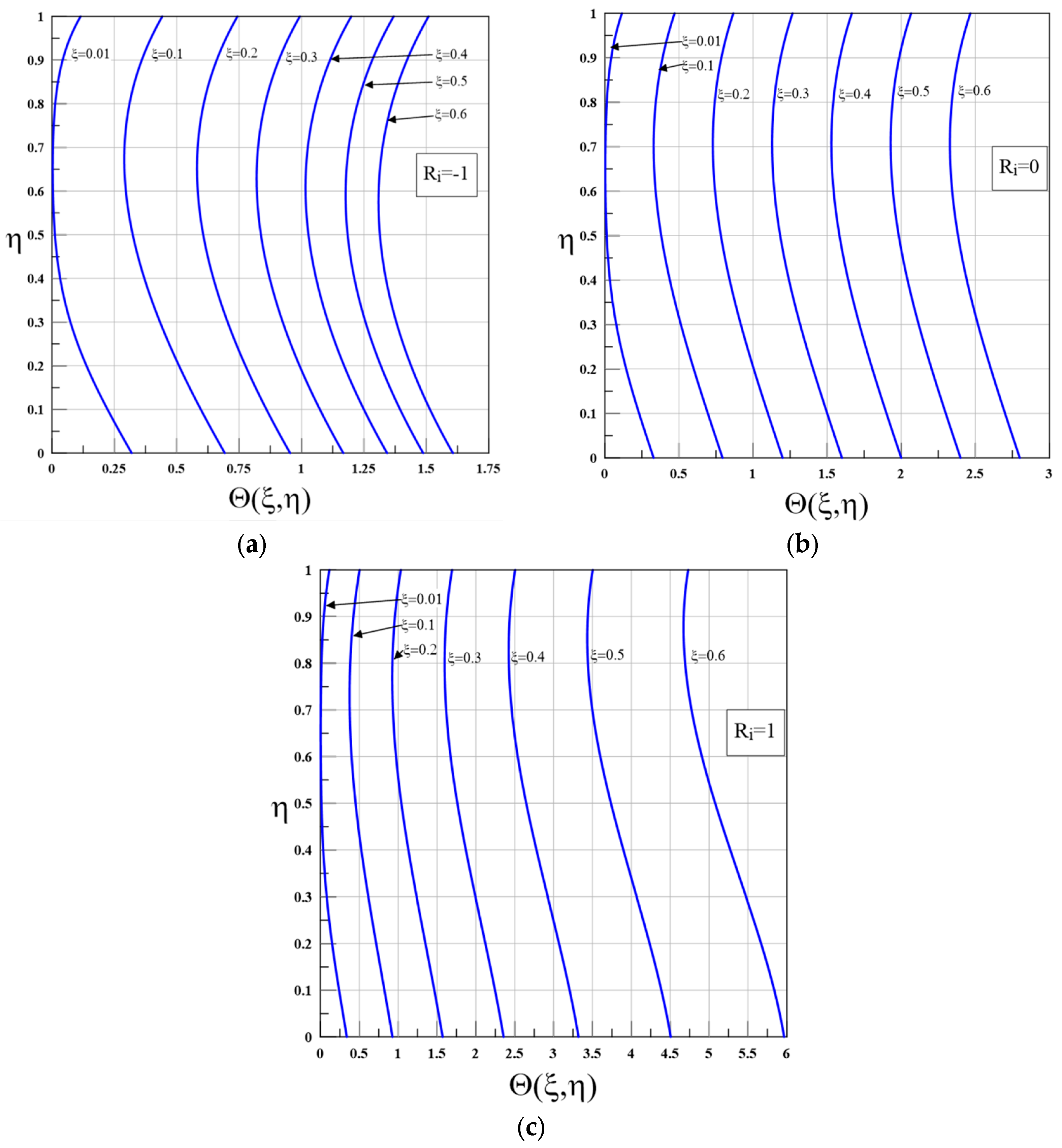
Figure 7a–c present the transverse distributions of the dimensionless temperature $\mathsf{\Theta }(\mathsf{\xi },\mathsf{\eta })$ versus the scaled wall-normal coordinate $\mathsf{\eta }$ for various streamwise positions $\mathsf{\xi }$ under symmetric Flux–Flux boundary conditions. The three subfigures compare the effects of buoyancy quantified by the Richardson number ${\mathrm{R}}_{\mathrm{i}}$: (a) ${\mathrm{R}}_{\mathrm{i}}=-1$ (unstable stratification), (b) ${\mathrm{R}}_{\mathrm{i}}=0$ (neutral forced convection), and (c) ${\mathrm{R}}_{\mathrm{i}}=1$ (stable stratification). In each case, the family of curves progresses from right to left as $\mathsf{\xi }$ increases, reflecting the physical evolution of the thermal field downstream. The rightmost curve $(\mathsf{\xi }\to 0)$ represents the entrance region, where conduction dominates and the thermal boundary layer is thin. As $\mathsf{\xi }$ increases, the profiles shift leftward, indicating boundary layer growth and the transition to advection-influenced heat transfer. The leftmost curve $(\mathsf{\xi }\gg 1)$ corresponds to the fully developed region, where advection and conduction are in balance, resulting in a flatter, parabolic profile. This right-to-left progression clearly illustrates the downstream maturation of the temperature field from conduction-controlled entrance flow to advection-balanced fully developed flow in stratified Couette systems.

Figure 7. Temperature profiles $\mathit{\Theta }(\xi ,\eta )$ at various $\xi$: (a) $R_i=-1$ (destabilizing); (b) $R_i=0$ (neutral); (c) $R_i=1$ (stabilizing).

In Figure 7a, corresponding to unstable stratification ($R_i=-1$), buoyancy reinforces the shear and accelerates vertical mixing. The rightmost profile (smallest $\xi = 0.01$) represents the thermal entrance region. It starts at $\mathit{\Theta } = 0.32$ near $\eta =0$ and decreases steeply, reaching $\approx 0.01$ at $\eta \approx 0.5$ and $\approx 0.11$ at $\eta =1$. As $\xi$ increases to $0.1-0.3$, the profiles flatten (maximum $\mathit{\Theta } \approx 0.32-0.84$) and shift leftward, showing rapid merging of the opposing thermal layers and early attainment of convective equilibrium. At $\xi = 0.6$, $\mathit{\Theta }$ peaks near $1.31$ with an almost linear gradient across $\eta$, indicating efficient heat redistribution and a very short thermal entrance length. This behavior evidences how destabilizing buoyancy enhances transport, reduces wall-to-wall temperature differences, and promotes a well-mixed core.

Figure 7b illustrates the neutral case ($R_i=0$), representing pure forced convection without buoyancy influence. The entrance profile $(\xi =0.01)$ exhibits pronounced curvature, starting from $\mathsf{\Theta }\approx 0.32$ at the flux-heated lower wall $(\eta =0)$—characteristic of a conduction-dominated entry flow under constant heat flux. This initial non-zero wall temperature results from the constant flux boundary condition, which dictates rapid near-wall heating before advection dominates downstream. As ξ increases (0.1–0.3), the profiles move leftward with smaller peaks, as the thermal boundary layers thicken symmetrically and begin to merge. At $\xi = 0.4-0.6$, the distribution approaches a parabolic shape with moderate values at the top wall, indicating the fully developed regime where advection and conduction reach equilibrium and heat transfer remains uniform between the two walls.

In Figure 7c, for stable stratification ($R_i=1$), buoyancy opposes the shear, inhibiting convective motion and delaying thermal development. The entrance profile decreases abruptly near the bottom wall before plateauing toward the top, creating a step-like shape with steep gradients near the walls and a nearly isothermal cold core. As the flow progresses downstream, the profiles flatten slowly with persistently high maximum values, reflecting weak heating in the core and sustained stratification. Even far downstream, the temperature remains low with sharp gradients confined to the walls, confirming that stabilizing buoyancy suppresses mixing, confines heat to boundary layers, and maintains a diffusion-dominated core even far downstream.

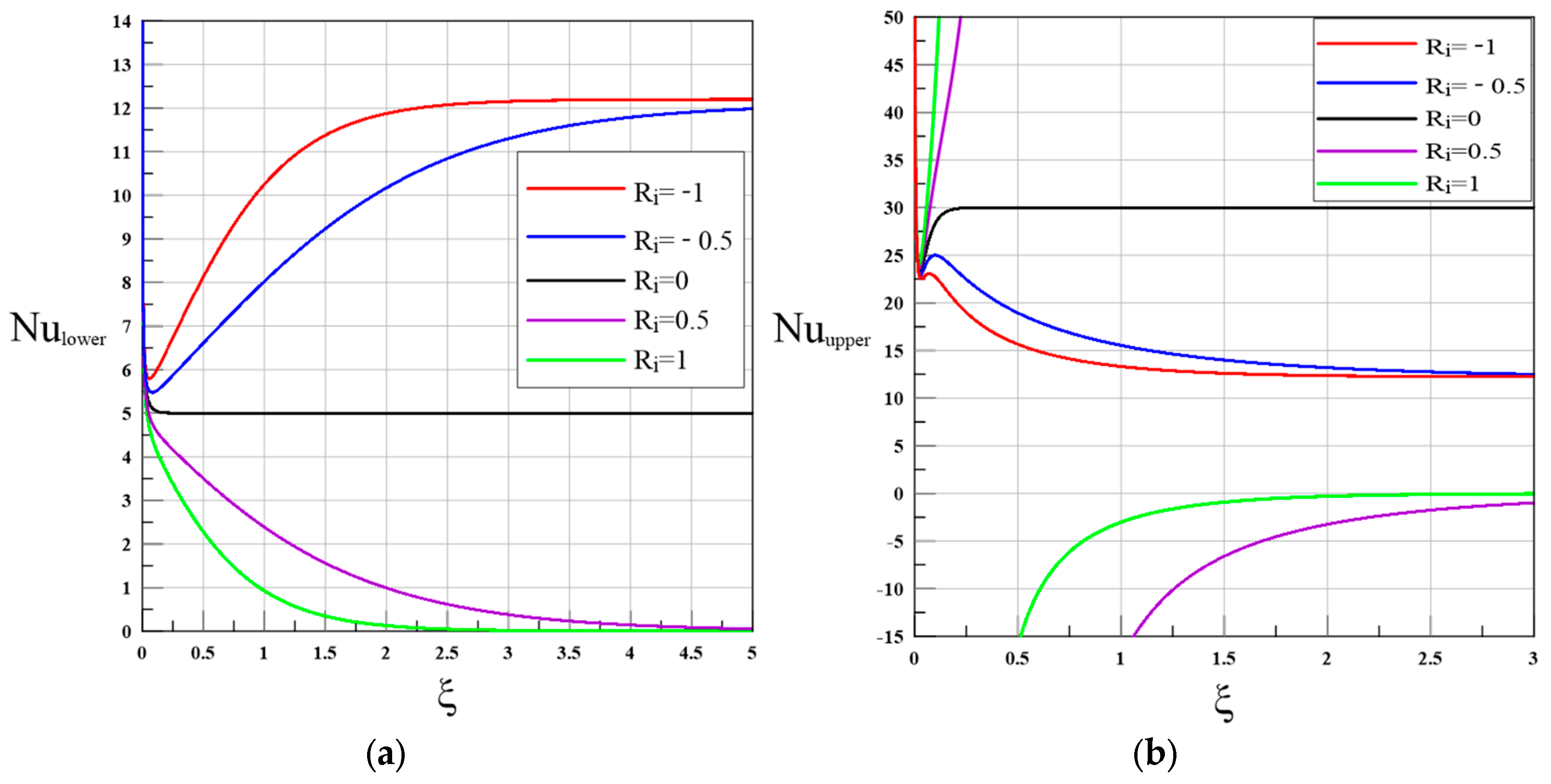
Figure 8a,b illustrate the longitudinal evolution of the local Nusselt numbers for the lower (${Nu}_{lower}$) and upper (${Nu}_{upper}$) walls as functions of the dimensionless axial coordinate $\xi$, under uniform heat flux (flux–flux) boundary conditions. The results are shown for five Richardson numbers $R_i=-1,-0.5,0,0.5,1$, which quantify the relative importance of buoyancy to forced convection. Negative $R_i$ values correspond to unstable stratification, where buoyancy acts in the same direction as shear and enhances mixing; positive $R_i$ values represent stable stratification, where buoyancy opposes shear and suppresses convective transport; $R_i=0$ denotes the pure forced convection limit.

Figure 8. Local Nusselt number for different values of $R_i$: (a) ${Nu}_{lower}$; (b) ${Nu}_{upper}$.

In Figure 8a, all curves start from nearly the same initial value of ${Nu}_{lower}\approx 14$ near $\xi =0$, a region dominated by thermal entrance effects where conduction prevails. Under unstable stratification ($R_i<0$), the Nusselt number rises sharply in the early region ($\xi \approx 0–2$) as buoyancy accelerates near-wall flow, intensifying upward transport of warm fluid and turbulent-like mixing in the lower boundary layer. At $R_i=-1$, ${Nu}_{lower}$ approaches an asymptotic value near $12.2$ beyond $\xi \approx 3$; for $R_i=-0.5$, the asymptotic value is slightly lower ($\approx 12.1$). This sustained enhancement confirms that destabilizing buoyancy thins the thermal boundary layer and strengthens wall temperature gradients, increasing convective heat removal. In the neutral case ($R_i=0$), ${Nu}_{lower}$ remains almost constant around $5$, indicating a hydrodynamically developed forced convection regime where wall-to-fluid heat transfer depends mainly on viscous shear rather than density stratification. For stable stratification ($R_i>0$), the opposite trend occurs: buoyancy acts counter to shear, suppressing vertical motion and thickening the thermal boundary layer. Consequently, ${Nu}_{lower}$ decreases steadily; for $R_i=0.5$, it drops below $1$ at $\xi \approx 2$; for $R_i=1$, it approaches $0$ as $\xi \to 5$. Heat transfer near the lower wall thus becomes almost purely diffusive, with minimal convective contribution due to strong flow stabilization.

Figure 8b reveals a more complex and asymmetric evolution of ${Nu}_{upper}$, governed by the interaction between buoyancy and the upward wall heating. For unstable stratification ($R_i<0$), buoyancy assists upward motion, concentrating hot fluid near the upper wall. As a result, ${Nu}_{upper}$, exhibits very high entrance values: about $67$ for $R_i<0$. The strong convective transport enhances wall temperature gradients, producing intense local heat fluxes. As the flow develops downstream, these gradients reduce, and ${Nu}_{upper}$ gradually decays toward $12.34–13.19$ beyond $\xi \approx 2$, indicating a transition toward a thermally developed convective regime. For the neutral case ($R_i=0$), ${Nu}_{upper}$ stays nearly constant to the value $30$ along the streamwise direction, demonstrating the expected thermal symmetry between the two walls under purely forced convection. In stable stratification ($R_i>0$), the upper-wall Nusselt number, ${Nu}_{upper}$, exhibits pronounced singularities arising from buoyancy forces that oppose wall heating. These singularities occur at specific streamwise positions ${\xi }_s$, where the wall temperature ${\mathit{\Theta }}_w\left(\xi \right)$ equals the bulk temperature ${\mathit{\Theta }}_b\left(\xi \right)$. At such points, the driving temperature difference for wall heat transfer momentarily vanishes, causing the denominator in the Nusselt number definition to approach zero. As a result, ${Nu}_{upper}\left(\xi \right)$ undergoes an apparent divergence and a sign reversal, reflecting a transient cancellation and inversion of the wall-to-fluid heat flux direction. These singularities gradually disappear in the fully developed regime ($\xi \to \infty$), where ${Nu}_{upper}\left(\xi \right)$ asymptotically approaches a finite constant value.

3.3. Implications for Climate Modeling and Sustainability

The present deep PINN framework offers a scalable, mesh-free alternative to DNS/LES for parameterizing buoyancy-affected heat transfer in stratified boundary layers. For stable stratification ($R_i>0$), suppressed $Nu$ and thickened thermal layers suggest reduced vertical heat flux in oceanic thermoclines and ABLs, potentially mitigating marine heatwave intensity under global warming. Conversely, destabilizing buoyancy ($R_i<0$) enhances mixing and $Nu$, promoting carbon sequestration via increased ${\mathrm{C}\mathrm{O}}_2$ uptake at the ocean surface.

With computational cost $5–10\times$ lower than traditional CFD, this PINN enables real-time subgrid-scale modeling in GCMs, improving projections of heat and mass exchange under climate change. These findings directly support SDG 13 (Climate Action) by providing an energy-efficient, high-fidelity tool for sustainable climate modeling.

4. Conclusions

This study successfully demonstrates the efficacy of deep Physics-Informed Neural Networks (PINNs) in modeling stratified forced convection heat transfer within plane Couette flows, tailored for atmospheric and oceanic boundary layers under climate change scenarios. By incorporating buoyancy effects through the Richardson number $(R_i\in [-1,1\left]\right)$, the model accurately captures nonlinear dynamics—including thermal boundary layer evolution, Nusselt number modulation, and gradient inversions—with relative $L_2$ errors below $0.009\%$ and $L_{\infty }$ errors below $0.023\%$ against analytical solutions ($R_i=0$) and high-order RK4 numerical solutions ($R_i\ne 0$). Results are valid within the linear velocity framework and may not capture coupled velocity–temperature dynamics in more general stratified flows. Future extensions to fully coupled PINNs will address this limitation.

Key findings include:

➢

In isolated-flux conditions, stable stratification ($R_i>0$) thickens boundary layers and significantly reduces $Nu$ (by up to $100\%$ across the domain), inducing singularities from heat flux reversals.

➢

Flux–flux cases show marked asymmetry under stratification: Stable stratification ($R_i>0$) delays development and suppresses mixing, driving $Nu$ toward zero. Conversely, unstable stratification ($R_i<0$) enhances vertical mixing, resulting in $Nu$ increasing markedly (by up to $140\%$) at the lower wall, while decreasing at the upper wall due to rapid homogenization.

➢

These stem from buoyancy–inertia interactions, where stable $R_i$ reduces vertical motion, akin to oceanic thermoclines, while unstable $R_i$ drives strong, asymmetric convective transport.

Novel contribution: This work introduces the first deep PINN capable of robust, high-accuracy simulation of stratified, buoyancy-coupled Couette flow across $R_i\in [-1,1]$, overcoming standard PINN failure through architectural and training innovations. The approach’s novelty—deep architecture with residuals, curriculum learning, and adaptive collocation—overcomes standard PINN limitations, achieving robust convergence for stiff high-$R_i$ systems. Climate-wise, this underscores warming-induced stratification’s role in amplifying heat trapping, reducing carbon fluxes, and intensifying extremes (SDG 13).

Future directions involve extending to turbulent regimes (using Reynolds-Averaged Navier–Stokes (RANS) or LES models), integrating salinity for double-diffusive effects, and hybridizing with GCMs for RCP8.5 projections. This framework paves the way for sustainable, data-efficient climate modeling, reducing computational barriers for global projections.

References

1. IPCC. Climate Change 2021: The Physical Science Basis; Cambridge University Press: Cambridge, UK, 2021. [Google Scholar]
2. Cheng, L.; Li, G.; Long, S.M.; Li, Y.; von Schuckmann, K.; Trenberth, K.E.; Mann, M.E.; Abraham, J.; Du, Y.; Cheng, X.; et al. Ocean stratification in a warming climate. Nat. Rev. Earth Environ. 2025, 6, 637–655. [Google Scholar] [CrossRef]
3. Deardorff, J.W. Numerical Study of Three-Dimensional Turbulent Channel Flow at Large Reynolds Numbers. J. Fluid Mech. 1970, 41, 453–480. [Google Scholar] [CrossRef]
4. Pope, S.B. Turbulent flows. Meas. Sci. Technol. 2001, 12, 2020–2021. [Google Scholar] [CrossRef]
5. Sullivan, P.P.; McWilliams, J.C. Dynamics of Winds and Currents Coupled to Surface Waves. Annu. Rev. Fluid Mech. 2010, 42, 19–42. [Google Scholar] [CrossRef]
6. Schneider, T.; Teixeira, J.; Bretherton, C.; Brient, F.; Pressel, K.G.; Schär, C.; Siebesma, A.P. Climate Goals and Computing the Future of Clouds. Nat. Clim. Change 2017, 7, 3–5. [Google Scholar] [CrossRef]
7. Monin, A.S.; Obukhov, A.M. Basic Laws of Turbulent Mixing in the Surface Layer of the Atmosphere. Tr. Geophiz. Inst. SSSR 1954, 24, 163–187. [Google Scholar]
8. Turner, J.S. Buoyancy Effects in Fluids; Cambridge University Press: Cambridge, UK, 1979. [Google Scholar]
9. Miles, J.W. On the Stability of Heterogeneous Shear Flows. J. Fluid Mech. 1961, 10, 496–508. [Google Scholar] [CrossRef]
10. Howard, L.N. Note on a Paper of John W. Miles. J. Fluid Mech. 1961, 10, 509–512. [Google Scholar] [CrossRef]
11. Bugeat, B.; Boldini, P.C.; Hasan, A.M.; Pecnik, R. Instability in Strongly Stratified Plane Couette Flow with Application to Supercritical Fluids. J. Fluid Mech. 2024, 984, A31. [Google Scholar] [CrossRef]
12. Michiyoshi, I.; Kikuchi, Y. Buoyancy Effects on Forced Convection Flow and Heat Transfer. Mem. Fac. Eng. Kyoto Univ. 1969, 31, 363–380. [Google Scholar]
13. Madhusudanan, A.; Illingworth, S.J.; Marusic, I.; Chung, D. Navier-Stokes–based linear model for unstably stratified turbulent channel flows. Phys. Rev. Fluids 2020, 7, 044601. [Google Scholar] [CrossRef]
14. Richardson, H.; Basu, S.; Holtslag, A.A.M. Improving stable boundary-layer height estimation using a stability-dependent critical bulk Richardson number. Bound.-Layer Meteorol. 2013, 148, 93–109. [Google Scholar] [CrossRef]
15. Incropera, F.P. Buoyancy effects in double-diffusive and mixed convection flows. In International Heat Transfer Conference Digital Library; Begel House Inc.: Danbury, CT, USA, 1986. [Google Scholar]
16. Townsend, A.A. Natural convection in the earth’s boundary layer. Q. J. R. Meteorol. Soc. 1962, 88, 51–56. [Google Scholar] [CrossRef]
17. Fornarelli, F.; Lippolis, A.; Oresta, P. Buoyancy Effect on the Flow Pattern and the Thermal Performance of an Array of Circular Cylinders. J. Heat Transf. 2017, 139, 022501. [Google Scholar] [CrossRef]
18. Raissi, M.; Perdikaris, P.; Karniadakis, G.E. Physics-Informed Neural Networks: A Deep Learning Framework for Solving Forward and Inverse Problems Involving Nonlinear Partial Differential Equations. J. Comput. Phys. 2019, 378, 686–707. [Google Scholar] [CrossRef]
19. Karniadakis, G.E.; Kevrekidis, I.G.; Lu, L.; Perdikaris, P.; Wang, S.; Yang, L. Physics-Informed Machine Learning. Nat. Rev. Phys. 2021, 3, 422–440. [Google Scholar] [CrossRef]
20. He, Y.; Yang, X. A physics-informed deep learning framework for estimating thermal stratification in a large deep reservoir. Water Resour. Res. 2025, 61, e2025WR040592. [Google Scholar] [CrossRef]
21. Ali, L.; Manan, A.; Ali, B. Maxwell Nanofluids: FEM Simulation of the Effects of Suction/Injection on the Dynamics of Rotatory Fluid Subjected to Bioconvection, Lorentz, and Coriolis Forces. Nanomaterials 2022, 12, 3453. [Google Scholar] [CrossRef]
22. Wang, S.; Teng, Y.; Perdikaris, P. Understanding and Mitigating Gradient Flow Pathologies in Physics-Informed Neural Networks. SIAM J. Sci. Comput. 2021, 43, A3055–A3081. [Google Scholar] [CrossRef]
23. Bengio, Y.; Louradour, J.; Collobert, R.; Weston, J. Curriculum Learning. In Proceedings of the 26th Annual International Conference on Machine Learning, Montreal, QC, Canada, 14–18 June 2009; Volume 41, pp. 41–48. [Google Scholar]
24. Raissi, M. Deep Hidden Physics Models: Deep Learning of Nonlinear Partial Differential Equations. J. Mach. Learn. Res. 2018, 19, 1–24. [Google Scholar]
25. Zhang, S.; Sun, C. Twin Forces: Similarity between Rotation and Stratification Effects on Wall Turbulence. J. Fluid Mech. 2024, 979, A45. [Google Scholar] [CrossRef]
26. Gebhart, B.; Jaluria, Y.; Mahajan, R.L.; Sammakia, B. Buoyancy-Induced Flows and Transport; Hemisphere Publishing Corporation: New York, NY, USA, 1988. [Google Scholar]
Disclaimer/Publisher’s Note: The statements, opinions and data contained in all publications are solely those of the individual author(s) and contributor(s) and not of MDPI and/or the editor(s). MDPI and/or the editor(s) disclaim responsibility for any injury to people or property resulting from any ideas, methods, instructions or products referred to in the content.
Article Metrics
Citations
Article Access Statistics
Multiple requests from the same IP address are counted as one view.