A Finite Element Method for Compressible and Turbulent Multiphase Flow Instabilities with Heat Transfer

Abstract

We present a new finite element framework for modeling compressible, turbulent multiphase flows with heat transfer. For two-fluid systems with a free surface, the Volume of Fluid (VOF) method is implemented without the need for interface reconstruction, while turbulence is resolved using a dynamic Vreman large eddy simulation (LES) model. Unlike most two-phase VOF studies, which neglect heat transfer, the present approach incorporates energy transport equations within the VOF formulation to account for heat exchange, an effect particularly important in turbulent flows. Conjugate heat transfer is often challenging in finite volume methods, which require explicit specification of heat fluxes at the solid–fluid interface, limiting accuracy and predictive capability. By contrast, the finite element formulation does not require heat flux inputs, allowing more accurate and robust simulation of heat transfer between solids and fluids. The method is demonstrated through three representative cases. First, a two-fluid instability with a single-mode perturbation is simulated and validated against analytical growth rates. Second, conjugate heat transfer is examined in a high-temperature flow over a cold metal cylinder, with validation performed both quantitatively—via pressure coefficient comparisons with experimental data—and qualitatively using vector field topology. Finally, compressible spray injection and breakup are modeled, demonstrating the ability of the framework to capture interfacial dynamics and atomization under turbulent, high-speed conditions. In the compressible spray injection and breakup case, the results indicate that the finite element formulation achieved higher predictive accuracy and robustness than the finite-volume method. With the same mesh resolution, the FEM reduced the root mean square error (RMSE) and mean absolute percentage error (MAPE) from 6.96 mm and 26.0% (for the FVM) to 4.85 mm and 12.7%, respectively, demonstrating improved accuracy and robustness in capturing interfacial dynamics and heat transfer. The study also introduced vector field topology to visualize and interpret coherent flow structures and instabilities, offering insights beyond conventional scalar-field analyses.

1. Introduction

Multiphase heat transfer in a turbulent and complex domain has been the subject of ample research, which exists in many applications such as the injection of liquid fuel into an internal combustion engine [1,2,3,4,5,6]. In two-fluid flows with a free surface, the interface separating the two fluids undergoes continuous distortion, which may cause surface breaking or coalescence of these two surfaces [7,8,9]. A popular approach to tackling these problems was to utilize an Euler mesh and allow the interface to move within the mesh [10]. There are two commonly used color functions, the volume-of-fluid (VOF) and level set functions, for tracking and locating interfaces [10,11,12]. In these methods, the entire domain of differing fluids is treated as a single mixture, with material properties aggregated according to the relative weighting within an element, as determined by the solution of the tracking function, which is represented by a color value.

When significant disparities exist between fluid material properties at the interface, the numerical representation of the system suffers from a lack of suitable methods to capture these disparities, leading to numerical instabilities during the solution. Smoothing techniques or interface reconstruction provide a method to overcome the disparities, although not ideal, and are necessary to address the instability problem that occurs during the simulation of the modeled equations. Particularly, the VOF method was widely used to deal with heat transfer across the interface separating two immiscible fluids, e.g., gas-liquid two-phase flows [13,14,15,16]. In the FV frame, VOF is always accompanied by interface reconstruction; hence, the temperature at the interface and the heat flux through it can be calculated in a way such that the continuity of the two properties at the contact surface is satisfied explicitly. In the proposed study, we combine VOF with FEM and show that interface reconstruction was not required to produce accurate solutions. A dynamic Vreman LES model was incorporated with VOF in the turbulence model [17]. In many applications with VOF, incompressible flow was assumed [13], where the energy was uncoupled from the fluid’s momentum solution, and the internal energy of the respective fluids was often constant. For many realistic problems, that assumption cannot be employed. Our system for solving fluid dynamics employs VOF for compressible and turbulent flows, capturing both mass transfer (mass flux) at the interface and heat transfer between the fluids.

As part of an effort to model heat transfer in multiphase systems where liquid spray may be quenching metal walls or otherwise wetting hot walls and evaporating or condensing vapors, we have applied the FEM system to solve the conjugate heat transfer (CHT) between fluids, gases, and solids. Many approaches have been proposed to model CHT. For example, coupled FEM with weak form meshless methods such as element free Galerkin (EFG) method or a meshless local Petrov-Galerkin (MLPG) method, and the most common was the finite volume systems [18]. These finite volume systems must approximate the flux from an assumed heat transfer coefficient and also use iteration until the heat flux is balanced. The system developed utilizes FEM for both fluid and solid, where the weakened form automatically conserves the flux between the materials since separate elements represent them, and therefore no assumption was made about the efficacy of the heat transfer (coefficient of heat transfer), nor are iterations required to conserve the flux [19]. The solid and gaseous materials are both identified on the computational grid, and at the interface, they share nodes. When solving for heat conduction in the solid, the shared nodes have the properties assigned to the solid. The same consistency was true when solving for the fluids. This method requires identifying the interface between the fluid and the solid. Like all other coupled FEM and meshless method, the nodes for fluid and the nodes for solids are placed to coincide with each other. Because of the weak formulation from FEM, the heat or mass flux was preserved on the interface so that it eliminates the need to assume for heat flux coefficient on the interface. This method is more accurate and also costs less computational time. A benchmark problem was presented, demonstrating the effectiveness of the CHT scheme.

In recent years, multiphase flow modeling has expanded well beyond traditional VOF and FEM strategies, with several numerical and hybrid approaches being actively explored. Coupled VOF–finite volume methods remain the standard for many compressible two-phase flow problems, particularly when interface reconstruction and adaptive meshing are required [20,21,22]. At the mesoscale, lattice Boltzmann methods (LBM) provide a kinetic-based alternative, which offers new ways to capture droplet breakup and coalescence [23]. Particle–mesh hybrids, such as smooth particle hydrodynamics (SPH) combined with finite element frameworks, have been applied successfully to simulate violent interfacial dynamics and conjugate heat transfer [24,25]. More recently, data-driven reduced-order models have emerged, where machine learning is used to accelerate spray and atomization simulations while preserving predictive accuracy [26,27]. In addition, higher-order compact finite-difference schemes have been successfully applied to non-premixed flame configurations, where their improved accuracy in resolving scalar transport and flamelet dynamics provides a useful benchmark for evaluating advanced multiphase and heat-transfer models such as the present FEM framework [28,29]. Together, the recent progress illustrates the growing diversity of tools available for multiphase flow problems, while also underscoring the need for unified frameworks that can handle compressible flow, turbulence, and conjugate heat transfer in a consistent manner.

Vector field topology is a powerful analysis technique that identifies the most essential structure of a vector field [30]. Its topological features include critical points and separatrices, which segment the domain into regions of coherent flow behavior, provide a sparse and semantically meaningful representation of the underlying data. In this paper, we utilize the open-source implementation from the Visualization Toolkit (VTK) to visualize our simulation results [31]. The vector-field topology is employed to go beyond conventional scalar or vortex-based visualization, extracting the underlying structure of the flow through critical points and separatrices. Tracking the evolution of these features provides a compact and physically meaningful picture of how instabilities form, propagate, and interact—for example, where Kelvin–Helmholtz rollers develop, Rayleigh-Taylor “mushroom” heads shed, or entrainment corridors emerge—offering new insights into the mechanisms driving turbulence and multiphase transport.

This study introduces a finite element framework for multiphase flow modeling by combining the volume-of-fluid (VOF) method with the finite element method (FEM) to avoid explicit interface reconstruction while preserving flux continuity across both fluid–fluid and fluid–solid boundaries. In contrast to finite volume or meshless approaches that require prescribed heat transfer coefficients and iterative balancing, the FEM framework inherently conserves fluxes through shared nodes, which provides improved accuracy in heat transfer predictions. In terms of numerical formulation, the present method combines different levels of accuracy for different operators to balance robustness and efficiency. Advection is handled using a Streamline Upwind Petrov-Galerkin (SUPG) formulation, which achieves third-order spatial accuracy [18], while diffusion and pressure terms are treated with standard Galerkin finite elements that are second-order accurate. Time advancement is carried out with a θ-method, giving second-order accuracy in time for the present simulations. Although the formal order may locally decrease near sharp phase interfaces due to boundedness requirements, the scheme maintains overall conservation and stability. For turbulence closure, the dynamic Vreman LES model by Waters et al. [17] was chosen for its robustness in compressible multiphase flows, where many alternative subgrid-scale models encounter stability challenges and difficulty in resolving interfacial dynamics. The novelty of the proposed framework lies in its unified treatment of compressible flow, interface-resolving VOF–FEM, and conjugate heat transfer. Validation is carried out through a set of canonical and application-driven cases, including three-dimensional Rayleigh-Taylor instability, conjugate heat transfer in cylinder flow, and spray injection dynamics.

2. Description of the Numerical Model

The standard 3D Navier–Stokes equations, as well as transport equations for mass, energy, and species (air/water vapor) conservation, are all solved for the Eulerian phase as the continuum. All governing equations are solved using the proposed new Conservative Predictor-Corrector solver and stabilized Petrov-Galerkin advection, as well as stabilized Pressure.

The transport equation governs the volume-of-fluid (VOF) formulation:

$${\displaystyle \frac{\partial f}{\partial t}}+U·\nabla f=0$$

(1)

where f is the volume of fluid and U is the velocity. Numerical diffusion in Equation (1) is controlled using the Streamline Upwind Petrov-Galerkin (SUPG) stabilization applied in the weak formulation. The SUPG weighting introduces a small amount of directional diffusion along the flow field to prevent oscillations while maintaining interface sharpness. No additional interface-compression or geometric reconstruction steps were required, since the finite-element formulation inherently maintains flux continuity and ensures mass conservation through the shared nodal connectivity of the mesh. The momentum equation reads:

$${\displaystyle \frac{{\rho }^{\mathrm{*}}{u}_i^{\mathrm{*}}-{\rho }^n{u}_i^n}{\mathsf{\Delta }t}}=-{\rho }^{n}U\nabla u_i+{\displaystyle \frac{\partial t_{ij}}{\partial x_j}}+{\displaystyle \frac{\partial {\tau }_{ij}}{\partial x_j}}+\sigma \kappa n{\delta }_{\Gamma }$$

(2)

where $u_i^{\mathrm{*}}$ is the intermediate velocity and ${\delta }_{\Gamma }$ is a Dirac Delta function at the interface. The term $\sigma \kappa n{\delta }_{\Gamma }$ represents the surface tension term. For sufficiently smooth interfaces, the identity $\nabla f=n{\delta }_{\Gamma }$ holds, where ${\delta }_{\Gamma }=\left|\nabla f\right|$ and $n=\nabla f/\left|\nabla f\right|$. In the weak finite-element form, the corresponding surface integral can be expressed equivalently as a volume integral,

$${\int }_{\Gamma }\delta \kappa n{\delta }_{\Gamma }\cdot v={\int }_{\Omega }\delta \kappa \nabla f\cdot v$$

(3)

which is valid throughout the volume domain. The interface normal and curvature are evaluated directly from the smoothed volume fraction field as n = ∇α/∣∇α∣ and κ = −∇⋅n. These quantities are computed using the same finite-element interpolation functions to ensure consistency and smooth gradients. Spurious currents are minimized by consistent treatment of the surface-tension force within the weak formulation, SUPG stabilization near the interface, and flux continuity across shared nodes—all of which maintain pressure stability and suppress artificial oscillations. Therefore, explicit interface tracking is not required to account for surface tension, although slight interface diffusion may occur depending on mesh resolution. In Equation (2), ${\tau }_{ij}=2\mu {\tilde{S}}_{ij}$ denotes the viscous stress of the filtered (resolved) field, with $\mu$ being the molecular (laminar) viscosity, and $t_{ij}$ denotes the subgrid-scale (SGS) stress tensor, modeled in the LES formulation as

$$t_{ij}-{\displaystyle \frac{1}{3}}{t}_{kk}{\delta }_{ij}=-2{\mu }_{sgs}({\tilde{S}}_{ij}-{\displaystyle \frac{1}{3}}{\tilde{S}}_{kk}{\delta }_{ij})$$

(4)

where ${\mu }_{sgs}$ is the subgrid-scale viscosity defined by the dynamic Vreman LES model [16], and ${\tilde{S}}_{ij}$ is the filtered strain-rate tensor. The resolved velocity field ${\tilde{u}}_i$ is used to compute the filtered strain-rate tensor. The dynamic Vreman LES model was employed to handle highly unsteady wall-bounded flows, ranging from laminar to fully turbulent. The subgrid viscosity ${\mu }_{SGS}$ is dynamically evaluated using a test filter and the Germano identity. This eliminates the need for empirical damping functions near walls, making it particularly effective for transitional multiphase flows with strong interface-driven turbulence. Previous validation has demonstrated accurate prediction of reattachment lengths in backward-facing step flows and shock–boundary layer interactions at high Mach numbers [17]. Implementation details and coefficients follow Waters, Carrington & Pepper [32], in which the model defines the SGS stress/heat flux at the grid and test scales and computes the dynamic coefficients from volume-averaged tensor products.

The pressure field was solved using a Poisson-type equation derived from the continuity constraint and the predictor-corrector velocity update, as given by

$${\displaystyle \frac{1}{c^2}}\mathsf{\Delta }P-\mathsf{\Delta }{t}^2{\theta }_1{\theta }_2{\displaystyle \frac{{\partial }^2\mathsf{\Delta }P}{\partial x_i^2}}=\mathsf{\Delta }{t}^2{\theta }_1{\displaystyle \frac{{\partial }^2\mathsf{\Delta }{P}^n}{\partial x_i^2}}-\mathsf{\Delta }t\left({\theta }_1{\displaystyle \frac{\partial \mathsf{\Delta }{u}_i^{\mathrm{*}}}{\partial x_i}}+{\displaystyle \frac{\partial {\rho }^n{u}_i^n}{\partial x_i}}\right)$$

(5)

Equation (5) is obtained by applying a predictor-corrector approach. First, an intermediate velocity is computed without the new pressure term. The continuity equation, discretized with a θ-scheme, is then enforced using the corrected velocity, ${\mathrm{u}}^{n+1}=u^{*}-∆t{\theta }_2\nabla (∆P)$. Using the weakly compressible relation ${\mathsf{\rho }}^{n+1}-{\mathsf{\rho }}^n=\left(1/C^2\right)∆P$ and substituting into the discretized continuity equation leads to the Poisson-type pressure equation shown in Equation (5). We also note that the associated momentum corrector, energy, and species transport formulations are presented in Equations (6)–(9). This addition makes the derivation consistent with the standard predictor-corrector framework and clarifies the role of the weighing parameters. When the flow was compressible the value of the sound speed was determined by $c=\sqrt{\gamma RT}$. When the solution method was for incompressible flow or when $f=1$, an artificial sound speed was used $c=\mathit{max}(\epsilon ,u_{conv},u_{diff})$ where $\epsilon$ is a number to ensure ‘$c$’ was not zero (here $u_{conv}$ was the flow velocity and $u_{diff}$ was the diffusive term). For VOF, pressure might not be continuous and averaging pressure on the interface was performed by using a control volume. A momentum correction was applied following the pressure update to enforce mass conservation.

$$\mathsf{\Delta }{U}_i=U^{n+1}-U^n={\mathsf{\Delta }U}^{\mathrm{*}}-\mathsf{\Delta }t{\displaystyle \frac{\partial P^{\prime }}{\partial x_i}}={\mathsf{\Delta }U}^{\mathrm{*}}-\mathsf{\Delta }t\left({\theta }_2{\displaystyle \frac{\partial \mathsf{\Delta }P}{\partial x_i}}+{\displaystyle \frac{\partial P^n}{\partial x_i}}\right)$$

(6)

Internal Energy transport was solved with energy in the form of temperature

$${\displaystyle \frac{\partial \tilde{E}}{\partial t}}=-{\displaystyle \frac{\partial }{\partial x_i}}\left(\tilde{E}{\tilde{u}}_i+p{\tilde{u}}_i\right)+{\displaystyle \frac{\partial }{\partial x_i}}\kappa {\displaystyle \frac{\partial \tilde{T}}{\partial x_i}}-{\displaystyle \frac{\partial \left(C_p{q}_i\right)}{\partial x_i}}+{\displaystyle \frac{\partial }{\partial x_i}}(t_{\mathit{ij}}+{\tau }_{ij})u_j$$

(7)

with the SGS heat flux defined as

$$q_j=-{\displaystyle \frac{{\mu }_{sgs}}{{Pr}_{sgs}}}{\displaystyle \frac{\partial \tilde{T}}{\partial x_j}}$$

(8)

where, $\kappa$ is the heat conductivity and $C_p$ is the specific heat capacity. The terms ${\mu }_{sgs}$ and ${Pr}_{sgs}$ represent the subgrid viscosity and the turbulent Prandtl number from the Vreman LES model. In this study, the value of $\kappa$ is different depending on the material, being solid or fluid thermal conductivity.

Species solution applies to gases species, that is, when it is given by the model equation.

$${\displaystyle \frac{\partial \overline{\rho }{\widetilde{\mathsf{{\rm Y}}}}_j}{\partial t}}=-{\displaystyle \frac{\partial }{\partial x_i}}\left(\overline{\rho }{\tilde{u}}_i{\widetilde{\mathsf{{\rm Y}}}}_j\right)+{\displaystyle \frac{\partial }{\partial x_i}}\overline{\rho }\left[\left(D_{j,N}+{\displaystyle \frac{{\mu }_{sgs}}{{Sc}_t}}\right){\displaystyle \frac{\partial {\widetilde{\mathsf{{\rm Y}}}}_j}{x_i}}\right]+\overline{\rho }{\widetilde{\mathsf{{\rm Y}}}}_j{f}_j\left(x_i\right)$$

(9)

where ${\mathsf{{\rm Y}}}_j={\displaystyle \frac{{\rho }_j}{{\rho }_{gas}}}$ is the mass fraction of the jth species. Gas properties are formed in aggregate from the mass fraction.

2.1. Implicit Solution Method

Developing an implicit solution scheme allows for a larger time step size and can add stability to model equations. It can be noted that an implicit method allows for larger time steps but would only maintain accuracy if spatial errors are larger than temporal errors. In this system, only advection and source terms are used for the load vector. For notational simplicity, superscripts and source terms are omitted in the following formulation.

$${\rho }^n{u}_i^{\mathrm{*}}-\mathsf{\Delta }t\times \left({\displaystyle \frac{\partial t_{ij}^{\mathrm{*}}}{\partial x_j}}-{\displaystyle \frac{\partial {\tau }_{ij}^{\mathrm{*}}}{\partial x_j}}\right)={\rho }^n{u}_i^n-\mathsf{\Delta }t\times {\displaystyle \frac{\partial \left({\rho }^n{u}_i^n{u}_j^n\right)}{\partial x_j}}$$

(10)

where $u_i^{\mathrm{*}}$ is the intermediate velocity. Using the mass-conserving projection method described previously results in multiplying. $u_i^{\mathrm{*}}$ by ${\rho }^n$ to form $U_i^{\mathrm{*}}$, hence $\Delta U_i^{\mathrm{*}}=U_i^{\mathrm{*}}-U_i^n$, as usual in the semi-implicit projection.

After determining the pressure as stated earlier, the specific internal energy is solved in explicit form generally because the limiting value for the CFL or Fourier number under turbulent flow is typically not from the energy or species transport equations. Though sometimes the implicit solution is used if deemed necessary, and is given by

$$\begin{array}{cc}\hfill E^{n+1}& - \mathsf{\Delta }t\times {\displaystyle \frac{\partial }{\partial x_i}}\left({\displaystyle \frac{\kappa }{C_v}}{\displaystyle \frac{\partial E^{n+1}}{\partial x_i}}\right)-\mathsf{\Delta }t\times {\displaystyle \frac{\partial }{\partial x_i}}\left({\displaystyle \frac{C_p{\mu }_{sgs}}{{\mathit{Pr}}_{\mathit{sgs}}{C}_v}}{\displaystyle \frac{\partial E^{n+1}}{\partial x_i}}\right)\hfill \\ & \hspace{1em}\hspace{1em}\hspace{1em}\hspace{1em}=E^n-\mathsf{\Delta }t\times {\displaystyle \frac{\partial }{\partial x_i}}\left(E^n{u}_i^{n+1}+P^{n+1}{u}_i^{n+1}\right)\hfill \\ & \hspace{1em}\hspace{1em}\hspace{1em}\hspace{1em}+ \mathsf{\Delta }t\times {\displaystyle \frac{\partial }{\partial x_i}}\left(t_{ij}^{n+1}+{\tau }_{ij}^{n+1}\right)\hfill \end{array}$$

(11)

where $E^{n+1}={\rho }^n{e}^{n+1}$ and $e^{n+1}$ is the internal energy, and we can get the temperature $T^{n+1}$ with $T^{n+1}={\displaystyle \frac{e^{n+1}}{C_v}}$.

The species transport equations can be treated in a similar manner if an implicit formulation is deemed necessary; however, such treatment is seldom required in practice. Constructing and inverting the matrices for multiple species adds considerable computational effort. However, since turbulent diffusion usually overwhelms molecular diffusion, an explicit treatment is generally adequate for practical accuracy. The present formulation is semi-implicit, preserving matrix symmetry to enable efficient large-scale parallel computations and reduce the cost of preconditioning. This approach offers nearly an order-of-magnitude improvement in computational speed, while allowing time steps that are typically 100–1000 times larger, depending on the flow conditions. Additional details on this performance improvement are provided by Waters and Carrington [32].

The solution of species transport equations poses additional numerical challenges compared to the momentum equations, primarily due to dispersion-induced accuracy loss. The SUPG stabilization is therefore applied to suppress dispersion in the advection terms and enhance solution stability. In the SUPG method, the test function is modified as

$$W_i=N_i+{\displaystyle \frac{\alpha h_e}{{2u}_e}}(u_e·\nabla N_i)$$

(12)

where $N_i$ are the standard Galerkin shape functions, $h_e$ is the element size in the local streamline direction, $u_e$ is the average element velocity, and ${\alpha }_e=\coth \left({\displaystyle \raisebox{1ex}{$Pe$}\!\left/ \!\raisebox{-1ex}{$2$}\right.}\right)-{\displaystyle \raisebox{1ex}{$2$}\!\left/ \!\raisebox{-1ex}{$Pe$}\right.}$, $\mathrm{P}\mathrm{e}=\raisebox{1ex}{$\rho h_e\left|u_e\right|$}\!\left/ \!\raisebox{-1ex}{${2K}_e$}\right.$, with Pe the element Peclet number and K_e the effective diffusion coefficient. This Petrov-Galerkin formulation provides third-order spatial accuracy for advection terms [18]. The SUPG weighting introduces selective artificial diffusion aligned with the flow direction, effectively damping dispersive oscillations while retaining second-order spatial accuracy for linear elements. The SUPG approach therefore improves robustness and predictive reliability compared with traditional second-order central discretization, particularly in the presence of steep gradients.

2.2. FEM Formulation

The governing equations are formulated in their weak form within the FEM framework. To keep the presentation clear, we focus here on the weak formulation of the explicit solver; the corresponding implicit form can be derived in the same way. The weak form for the intermediate velocity, which includes the semi-implicit correction ΔU, is given as:

$$\begin{array}{cc}\hfill {\int }_{\mathsf{\Omega }}& \left\{N_i\right\}\left[N_j\right]\left\{\mathsf{\Delta }{\dot{U}}_i\right\}d\mathsf{\Omega }\hfill \\ & \hspace{1em}\hspace{1em}\hspace{1em}\hspace{1em}\hspace{1em}+{\int }_{\mathsf{\Omega }}\rho \left\{N_i\right\}\left[N_k\right]\left\{u_k\right\}\left[{\displaystyle \frac{\partial N_j}{\partial x_k}}\right]\left\{u_i\right\}d\mathsf{\Omega }\hfill \\ & \hspace{1em}\hspace{1em}\hspace{1em}\hspace{1em}\hspace{1em}-{\int }_{\mathsf{\Omega }}\left[\mathrm{\mu }+{\mathrm{\mu }}_t\right]\left\{{\displaystyle \frac{\partial N_i}{\partial x_j}}\right\}\left[\left[{\displaystyle \frac{\partial N_j}{\partial x_i}}\right]\left\{u_i\right\}-{\displaystyle \frac{2}{3}}{\delta }_{ij}\left[{\displaystyle \frac{\partial N_j}{\partial x_i}}\right]\left\{u_i\right\}\right]d\mathsf{\Omega }\hfill \\ & \hspace{1em}\hspace{1em}\hspace{1em}\hspace{1em}\hspace{1em}-{\int }_{\mathsf{\Omega }}\left\{N_i\right\}\left(\left[N_k\right]\left\{P_i\right\}\right)\left\{u_i\right\}d\mathsf{\Omega }\hfill \\ & \hspace{1em}\hspace{1em}\hspace{1em}\hspace{1em}\hspace{1em}+{\int }_{\mathsf{\Omega }}\rho \left\{N_i\right\}f\left\{x_i\right\}d\mathsf{\Omega }-{\int }_{\mathsf{\Gamma }}\left\{N_i\right\}\left[\mathrm{\mu }+{\mathrm{\mu }}_t\right]n_j\left[{\displaystyle \frac{\partial N_j}{\partial x_i}}\right]\left\{U_i\right\}d\Gamma =0\hfill \end{array}$$

(13)

where $f\left(x_i\right)$ is the body force per unit mass.

The weak form of the pressure equation is obtained by multiplying the governing equation by the test function {$N_i$} and integrating over the domain $\mathsf{\Omega }$. This leads to

$$\begin{array}{c}{\displaystyle \frac{1}{{\mathrm{c}}^2}}{\int }_{\mathsf{\Omega }}(\left\{{\mathrm{N}}_{\mathrm{i}}\right\}\left[{\mathrm{N}}_{\mathrm{j}}\right]+\mathsf{\Delta }{\mathrm{t}}^2{\mathsf{\theta }}_1{\mathsf{\theta }}_2\left\{{\displaystyle \frac{\partial {\mathrm{N}}_{\mathrm{i}}}{\partial {\mathrm{x}}_{\mathrm{j}}}}\right\}\left[{\displaystyle \frac{\partial {\mathrm{N}}_{\mathrm{j}}}{\partial {\mathrm{x}}_{\mathrm{i}}}}\right])\left\{\mathsf{\Delta }{\mathrm{P}}_{\mathrm{i}}\right\}\mathrm{d}\mathsf{\Omega }\hfill \\ \hspace{1em}\hspace{1em}\hspace{1em}\hspace{1em}\hspace{1em}\hspace{1em}\hspace{1em} =\mathsf{\Delta }\mathrm{t}\left[{\int }_{\mathsf{\Omega }}\left[{\displaystyle \frac{\partial {\mathrm{N}}_{\mathrm{i}}}{\partial {\mathrm{x}}_{\mathrm{j}}}}\right]\{{\mathrm{N}}_{\mathrm{j}}\}\{{\mathrm{U}}_{\mathrm{i}}^{\mathrm{n}}\}\mathrm{d}\mathsf{\Omega }+{\mathsf{\theta }}_1{\int }_{\mathsf{\Omega }}\left[{\displaystyle \frac{\partial {\mathrm{N}}_{\mathrm{i}}}{\partial {\mathrm{x}}_{\mathrm{j}}}}\right]\{{\mathrm{N}}_{\mathrm{j}}\}\{\mathsf{\Delta }{\mathrm{U}}_{\mathrm{i}}^{\mathrm{*}}\}\mathrm{d}\mathsf{\Omega }\right]\hfill \\ \hspace{1em}\hspace{1em}\hspace{1em}\hspace{1em}\hspace{1em}\hspace{1em}\hspace{1em} -\mathsf{\Delta }\mathrm{t}{\mathsf{\theta }}_1{\int }_{\mathsf{\Omega }}\left\{{\displaystyle \frac{\partial {\mathrm{N}}_{\mathrm{i}}}{\partial {\mathrm{x}}_{\mathrm{j}}}}\right\}\left[{\displaystyle \frac{\partial {\mathrm{N}}_{\mathrm{j}}}{\partial {\mathrm{x}}_{\mathrm{i}}}}\right]\left\{{\mathrm{P}}_{\mathrm{i}}^{\mathrm{n}}\right\}\hfill \end{array}$$

(14)

The boundary integrals arising from the application of Green’s theorem are particularly advantageous for this formulation, as discussed by Zienkiewicz and Codina [33].

2.3. Weak Form of Conservation of the Internal Energy

We calculate the energy transport first without concern for the sources of spark ignition or chemical heat release from reactions. ‘$Q_c$’, or enthalpy changes from droplet evaporation ‘$Q_e$’ and are added mid-algorithm during the time step in which they are calculated. As mentioned, typically the energy equation is solved explicitly as follows: that is, we solve for the change in ‘E’ and then update the energy on each node.

$$\begin{array}{c}{\int }_{\mathsf{\Omega }}{c}_p\left\{N_i\right\}\left[N_j\right]\left\{{\dot{E}}_i\right\}d\mathsf{\Omega }\\ +{\int }_{\mathsf{\Omega }}\left\{N_i\right\}\left[N_k\right]\left\{u_k\right\}\left[{\displaystyle \frac{\partial N_j}{\partial x_k}}\right]\left\{E_i\right\}d\mathsf{\Omega }\\ -{\int }_{\mathsf{\Omega }}\left[\kappa +{\displaystyle \frac{{\mathrm{\mu }}_t}{{Pr}_i}}\right]\left\{u_k\right\}\left\{{\displaystyle \frac{\partial N_i}{\partial x_j}}\right\}\left[{\displaystyle \frac{\partial N_j}{\partial x_i}}\right]\left\{T_i\right\}d\mathsf{\Omega }\\ -{\int }_{\mathsf{\Omega }}\begin{array}{c}\left(\left\{{\displaystyle \frac{\partial N_i}{\partial x_j}}\right\}\left[\left[{\displaystyle \frac{\partial N_j}{\partial x_i}}\right]-{\displaystyle \frac{2}{3}}{\delta }_{ij}\left[{\displaystyle \frac{\partial N_j}{\partial x_i}}\right]\right]\left\{u_i\right\}\right)\left[N_j\right]\left\{u_k\right\}d\Omega \end{array}-{\int }_{\mathsf{\Omega }}\left\{N_i\right\}\left(\left[N_k\right]\left\{P_i\right\}\right)\left\{u_i\right\}d\mathsf{\Omega }\\ -{\int }_{\mathsf{\Omega }}\left\{N_i\right\}{Q}_{s}d\mathsf{\Omega }-{\int }_{\mathsf{\Gamma }}\left\{N_i\right\}\mathrm{n}·\left(\left[N_j\right]\left\{q_i\right\}\right)d\mathsf{\Gamma }=0\end{array}$$

(15)

where $N_i$ was the shape function on the $i_{th}$ node, Ω was the entire simulation domain and Γ was the boundary.

In Equation (15), the entire domain integral was the summation of all local element integral and the last term in Equation (15) was the surface integral of the entire domain. Therefore, there was no surface integral involved on the element surface, which makes conjugate heat transfer easier to deal with between the metal and fluid interface.

Heat transfer modeling with the FEM automatically conserves flux across elements/cells, as shown in Equation (14); hence, there is no need to iteratively determine flux conservation between materials when the surfaces are separated by element/cell sides. What must occur is that the nodes on these surfaces have material properties for both the solid and the fluid, using the solid properties by integrating over the solid element, and the fluid properties by integrating over the fluid element. So, for FEM integration, when the cell was a fluid Equation (7) was used, and when the cell was solid, the usual conduction equation (Equation (16)) was solved.

$${\displaystyle \frac{\partial {\rho }_s{C}_{p,s}{T}_s}{\partial t}}={\displaystyle \frac{\partial }{\partial x_i}}{\kappa }_s{\displaystyle \frac{\partial T}{\partial x_i}}$$

(16)

where ${\rho }_s$ was the solid density, $C_{p,s}$ was the heat capacity for solid, and ${\kappa }_s$ was the value of the solid’s thermal conductivity. Coupling Equations (7) and (16) within the finite element integration framework ensures a continuous heat flux across the solid–fluid interface, eliminating the need for any imposed flux assumptions and improving the overall accuracy of energy coupling. Noting that Equation (7) is solving for the internal energy, while Equation (16) is solving for temperature. To couple those two equations into one system, Internal Energy transport is solved with energy in the form of temperature

$${\displaystyle \frac{\partial (\rho C_{p}T)}{\partial t}}=-{\displaystyle \frac{\partial }{\partial x_i}}(\rho C_p{u}_{i}T+p{u}_i)+{\displaystyle \frac{\partial }{\partial x_i}}(\kappa +{\displaystyle \frac{{\mu }_{sgs}}{{\mathrm{Pr}}_{sgs}}}){\displaystyle \frac{\partial T}{\partial x_i}}+{\displaystyle \frac{\partial }{\partial x_i}}(t_{ij}+{\tau }_{ij})u_j$$

(17)

2.4. Spray Dynamics and Evaporation Modeling

In Case III, spray injection was modeled using a Kelvin–Helmholtz/Rayleigh-Taylor (KH–RT) approach to capture the transition from early injection to ligament breakup and droplet atomization. The injection process was represented with spherical “blob” droplets following the Reitz model [34], with parcels tracked in a Lagrangian framework that accounts for advection, turbulent diffusion, and evaporation. The study focuses on KH–RT with evaporation modeling, while additional treatments such as collision, wall-film formation, and splashing are available in the underlying framework [17,35]. In the two-phase model, liquid injection is represented by discrete particles that undergo successive breakup, atomization, and evaporation. Initial droplet size, velocity, and spray cone angle are defined from nozzle flow conditions, while subsequent dynamics account for drag, heat and mass transfer, and turbulent dispersion. Droplet interactions with turbulence are modeled through eddy lifetime criteria, with particles either dispersing or remaining trapped within local eddies [17].

Droplet evaporation is modeled under the assumption of spherical droplets, with evaporation driven by both thermodynamic equilibrium and convective heat and mass transfer. The formulation incorporates carrier-flow effects through correlations for heat and mass transfer coefficients, which depend on Reynolds, Prandtl, and Schmidt numbers, as described by Abramzon and Sirignano [36]. Transport properties such as viscosity, surface tension, and thermal conductivity are treated as temperature-dependent, while turbulent dispersion and advection are accounted for using a Lagrangian particle framework. Conservation of mass, momentum, and energy is maintained between the droplet phase and the surrounding gas, with latent heat of vaporization governing the phase change process.

2.5. Turbulence Modeling

A dynamic Vreman-type LES method, which can transition through laminar to fully turbulent flow, is adopted in the FEM model. It requires no assumptions about the turbulent sublayers near walls in bounded flows; this is ideal for cases where the turbulent wall layers are never in equilibrium and the flow is not always very turbulent. Unlike most turbulence models, e.g., direct numerical simulation (DNS) [28], this VM-LES model does not involve any explicit filtering, averaging, or clipping procedure to stabilize the numerical method, enabling it to be used in simulations of flows with complex geometries [17]. The LES handles the transition from laminar to fully turbulent flow in fluids/gases, as the system is highly unsteady.

In LES, turbulent motions smaller than the filter size Δ are removed by applying a spatial filter to the conservation equations of mass, momentum, and energy. The filtered variable $\overline{\varphi }$ is defined by

The resolved velocity field ${\tilde{u}}_i$ is used to compute the filtered strain-rate tensor:

$$\overline{\varphi }(x_j,t)={\int }_{D}G\left(x_j,{\acute{x}}_j\right)\varphi \left(x_j,{\acute{x}}_j\right)d{\acute{x}}_j$$

(18)

where G is the box or top-hat filter function and Δ represents the grid filter width, typically taken as the cubic root of the element volume in the finite-element framework. The Favre filtering of any variable $\varphi$ is expressed as $\tilde{\varphi }=\overline{\rho \varphi }/\overline{\rho }$. The Favre-filtered continuity and momentum equations govern the resolved large-scale eddies. The subgrid stress and heat flux are represented by Equation (4) and Equation (8), respectively.

In the fixed-coefficient Vreman model, the eddy viscosity is given by ${\mu }_{SGS}=\overline{\rho }{C}_{vm}{\mathsf{\Pi }}^g,$ where ${\mathsf{\Pi }}^g=\sqrt{{\beta }_{\beta }^g/\left({\alpha }_{ij}{\alpha }_{ij}\right)}$ and ${\beta }_{\beta }^g$ depends on velocity gradients invariants. However, to account for non-equilibrium and backscatter effects, a dynamic Vreman model is implemented here. The dynamic formulation applies a second test filter ($\hat{\mathsf{\Delta }}=2\mathsf{\Delta }$) and determines the local coefficient by minimizing the error between the resolved and test-filtered subgrid stresses using the Germano identity and the least square method [37]:

$${\mathrm{C}}_{DV}={\displaystyle \frac{{⟨{\mathrm{L}}_{ij}{\mathrm{M}}_{ij}⟩}_V}{{⟨{\mathrm{M}\mathrm{L}}_{ij}{\mathrm{M}}_{ij}⟩}_V}}$$

(19)

where angle brackets denote volume integration over the domain. This procedure adaptively evaluates the SGS viscosity field, improving accuracy in regions of strong flow gradients or unsteady shear layers. The dynamic SGS viscosity thus obtained ensures smooth transition from laminar to turbulent flow without artificial damping, making it particularly effective for complex multiphysics systems with strong interface-driven turbulence.

3. Results and Discussion

3.1. Case I: Classical Viscous Rayleigh-Taylor Instability

The classical case of 3D viscous Rayleigh-Taylor instability (RTI) [26] was studied, where the heavy fluid stands on the light fluid in a gravitational field directed downward along the vertical (Z) axis. Those two fluids were considered as incompressible in a bounded domain. The 3D Rayleigh-Taylor instability was selected as a canonical benchmark because it is a well-known test of interfacial mixing and buoyancy-driven turbulence. By exciting a single-mode perturbation, we can directly compare the early-time growth with analytical theory while also assessing whether the model captures the expected bubble-spike structures and transition to turbulence. The simulation was run for a sufficient amount of time to observe how the fluid responds to the wall. The domain’s dimensions were (−5 cm, 5 cm) × (−5 cm, 5 cm) × (0 cm, 40 cm), comprising 202,160 elements and 214,461 nodes.

The simulation was run with the density ratio of 3 to 1, where the Atwood number was A = 0.5. The variable time step was adjusted dynamically by the flow development to limit the maximum convective Courant-Friedrichs-Lewy (CFL) number to 0.5. On the top and base walls, non-slip boundary conditions were applied. Whereas on the four sides of the walls, periodic boundary conditions were considered. Here, we study the evolution of a 3D single-mode Rayleigh-Taylor instability by adding a perturbation on the interface z = 20: $\eta (x,y){=h}_0[\mathit{cos}(2\pi x/\lambda )+\mathit{cos}(2\pi y/\lambda \left)\right]$, where $h_0=0.1 \mathrm{cm}$ is the initial amplitude and $\lambda =10 \mathrm{cm}$ is the perturbation wavelength. A single-mode perturbation excites only one Rayleigh-Taylor mode, avoiding nonlinear mode coupling and allowing the instability amplitude to follow the classical linear growth rate, $h\left(t\right){=h}_0{e}^{\gamma t}and\gamma =\sqrt{Agk}$, where $k=2\pi /\lambda$ is the perturbation wavenumber, A is the Atwood number, and g is the gravitational acceleration. This setup provides a clean validation case, since the early-time growth can be directly compared with analytical predictions before nonlinear saturation develops. The initial set up was shown in Figure 1. The coupled VOF-FEM-LES framework was used to investigate Rayleigh-Taylor instability, using the dynamic Vreman LES model. This approach avoids the need to fully resolve the boundary layer while still capturing the key features of the instability with high accuracy. Figure 2 and Figure 3 showed the density development at different times on the X plane. It can be seen that at different times, the RT instability was well captured and the simulation can run long enough up to 3.0 s to see the heavy fluid reach the base while the light fluid went upwards Figure 3iv. The turbulent kinetic energy is shown in the density contour plot, where turbulent mixing is observed, and the bubble fluid motion is disrupted, as seen in Figure 2.

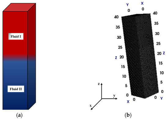
Figure 1. (a) Initial configuration for the classical viscous Rayleigh-Taylor (RT) instability showing two immiscible fluids, with fluid 1 (0.62 kg/m³) overlying fluid 2 (1.9 kg/m³). (b) Structured finite-element mesh used for the numerical simulation domain.

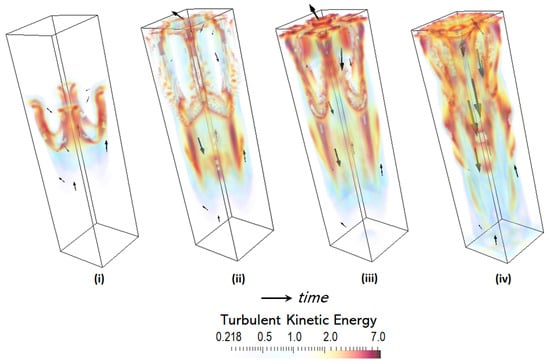
Figure 2. Transient evolution of the 3D turbulent kinetic energy contours illustrating the progressive development of the classical viscous Rayleigh-Taylor instability. The snapshots correspond to different time instants: (i) 1.2 s, (ii) 2.0 s, (iii) 2.10 s, and (iv) 2.40 s. The formation and growth of interfacial vortical structures are evident as the instability transitions from the linear to the nonlinear regime.

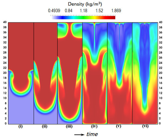
Figure 3. Transient evolution of the density contours on the YZ plane during the classical viscous Rayleigh-Taylor instability at successive times: (i) 1.2 s, (ii) 2.0 s, (iii) 2.10 s, (iv) 2.20 s, (v) 2.4 s, and (vi) 3.03 s. The results illustrate the progressive interface deformation, bubble-spike formation, and transition toward the nonlinear mixing regime.

The unstable interface diffuses into the light fluid and forms spikes. For the entire evolution interface in the RTI, the top of the bubble or spike represents the structure that grows fastest and has the longest amplitude. Hence, we investigate the time evolution of the amplitude of the spike or the penetration before the center bubble hits the bottom wall. The interface starts at $z=20 \mathrm{cm}$ and we normalize the amplitude as the $h/20$, where h was denoted as the amplitude. For a simple inviscid and incompressible case in a domain much larger than the perturbation wavelength, the perturbation at the interface grows exponentially with a rate $\gamma =\sqrt{Ag\kappa }$ where $g$ was the gravitational acceleration and $\kappa ={\displaystyle \frac{2\pi }{\lambda }}$. In this study, the gravitational acceleration is set to $g=0.5 \mathrm{m}/{\mathrm{s}}^2$.

As demonstrated in Figure 4, the numerical results closely match the analytical prediction during the initial, linear stage of the Rayleigh-Taylor instability, when the perturbation amplitude grows exponentially as expected. Once the disturbance reaches roughly 0.1λ, however, the growth begins to depart from the simple exponential law. Beyond this point, nonlinear mechanisms take over: spikes become narrower and accelerate under gravity, bubbles broaden and rise more quickly, and shear at the interface gives rise to secondary vortical structures [38]. These processes promote mixing and mode coupling, which drive the instability faster than the classical theory anticipates.

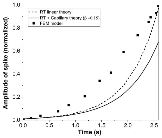
Figure 4. Comparison of normalized spike amplitude growth with time among the Rayleigh-Taylor (RT) linear theory, the combined RT + capillary theory (β = 0.15), and the finite element (FEM) simulation. The RT linear theory represents the classical exponential growth in the absence of surface tension effects, while the RT + capillary model incorporates capillary stabilization that moderates the growth rate.

To account for interfacial tension effects, the Rayleigh-Taylor + capillary theory modifies the linear growth rate of a single Fourier mode to

$${\mathsf{\gamma }}_{RT+cap}^2=Agk-{\displaystyle \frac{\sigma k^2}{\left({\rho }_1+{\rho }_2\right)}}=Agk\left(1-\beta \right),$$

(20)

where A is the Atwood number, k = 2π/λ is the wavenumber, σ is the surface tension coefficient, and

$$\beta ={\displaystyle \frac{\sigma k^2}{\left({\rho }_1+{\rho }_2\right)Ag}}$$

(21)

is a nondimensional capillary parameter (β = 0.15 in this study). This formulation predicts a slightly lower growth rate than the inviscid RT linear model, which reflects the stabilizing influence of surface tension on short-wavelength curvature. However, the FEM results in Figure 4 show closer agreement with the RT linear theory than with the RT + capillary model, indicating that under the present operating conditions, the effective capillary forces are relatively weak compared with buoyancy, while viscous diffusion and interface deformation dominate the dynamics. The deviation seen in Figure 4, therefore, marks the transition from linear to nonlinear behavior and highlights the ability of the FEM framework to resolve flow features beyond the reach of idealized analytical models.

The density evolution shown in Figure 3 provides a macroscopic view of how the Rayleigh-Taylor interface deforms over time and reveals the growth of bubbles and spikes as the heavy and light fluids interchange positions. This visualization clearly captures the large-scale structure of the instability and its transition toward a nonlinear mixing regime. In contrast, Figure 4 provides a quantitative view of spike amplitude growth, showing how the system gradually departs from the exponential trend predicted by linear theory as nonlinear effects begin to dominate. Whereas Figure 4 quantifies the spike amplitude growth, demonstrating how the system departs from the exponential trend predicted by linear theory as nonlinear effects become dominant. However, although these analyses depict the overall deformation and growth of the interface, they do not reveal the internal flow organization that drives these transitions.

To bridge this gap, a topological analysis of the velocity field was conducted using the open-source Visualization Toolkit (VTK), as illustrated in Figure 5. Unlike the density contours, which show only scalar field evolution, the topological framework exposes the structural dynamics of the flow—identifying critical points, separatrices, and invariant manifolds that delineate distinct regions of motion. All streamlines within a single segment share the exact origin and destination, so a repelling or attracting critical point in an incompressible slice corresponds to inflow or outflow from the plane. Although separatrices do not represent permanent barriers, they temporarily restrict transport and delineate the evolving organization of the flow field. As shown in Figure 5, the separatrices align closely with the evolving interface between the heavy and light fluids, highlighting their role as structural dividers of the Rayleigh-Taylor instability. As the instability develops, the topological structure becomes increasingly intricate: new critical points emerge, separatrices stretch and reconnect, and the underlying flow organization is continually reshaped. This progression marks the transition from a relatively ordered growth phase to a more chaotic state.

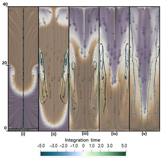
Figure 5. The transient profile of the topology of the RT instability on the YZ plane at (i) 1.2 s (ii) 2.10 s (iii) 2.20 s (iv) 2.40 s (v) 3.03 s. Critical points colored by type. Red: repelling, white: saddle, blue: attracting. The separatrices are colored by integration time starting at the corresponding saddle. The background visualizes the instantaneous velocity through Line Integral Convolution and the ratio of the fluids through color coding.

The separatrices form instantaneous transport boundaries across which mixing is inhibited, but not time-varying transport boundaries [31,39]. Such a structural perspective provides physical insight that goes well beyond what can be inferred from scalar density fields or velocity magnitudes alone. It exposes the birth and evolution of coherent vortical regions, the migration and eventual merging of separatrices that partition the flow, and the gradual erosion of symmetry that signals nonlinear mode coupling. The asymmetry evident in Figure 5iv is significant, it demonstrates that topological features can detect subtle deviations from idealized symmetric growth, thereby offering a mechanistic view of how small disturbances are amplified and ultimately drive the transition to turbulence.

3.2. Case II: Conjugate Heat Transfer in Flow over a Cylinder

For the second case study, a conjugate heat transfer (CHT) simulation was run for flow over a cylinder. The setup of the CHT simulation is shown in Figure 6, where a heated flow with a temperature of 600 K passes over a cold metal cylinder with an initial temperature of 373 K (Table 1). The cylinder temperature was not prescribed as constant but allowed to evolve dynamically under the influence of convective heat transfer, thereby capturing the coupled solid–fluid thermal interaction inherent to conjugate heat transfer. Non-slip boundary conditions and a fixed wall temperature of 600 K were applied along the outer sidewall and the inner surface of the metal boundary.

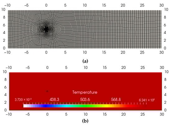
Figure 6. Computational setup for the conjugate heat transfer case: (a) 3D finite-element mesh distribution around the circular cylinder and (b) Y-axis slice showing the initial temperature field. The mesh is refined near the solid–fluid interface to accurately resolve the thermal boundary layer and capture the heat exchange between the cylinder and the surrounding flow.

Table 1. Boundary conditions for the conjugate heat transfer in flow over a cylinder (Case II).

	Fluid		Metal
Vf ρf kf	0.9 m/s 0.62 kg/m3 4.5 × 103 W/cm-K	ρm km	0.78 kg/m3 5 × 106 W/cm-K

For the test case, the inlet velocity was set to 0.9 m/s, which corresponds to a Reynolds number of 5 × 10³. This condition falls within the subcritical flow regime; the boundary layer remains laminar from the stagnation point at the front of the cylinder to the point where it separates. The separation of the boundary layer can be seen in Figure 7, where the velocity and turbulent kinetic energy (TKE) contours illustrate the onset of separation, the formation of a recirculation zone, and the gradual dissipation of turbulence downstream. The flow separation produces periodic pressure variations and forms a wake with alternating vortices downstream of the cylinder. To evaluate the predictive performance of the FEM model, the computed mean pressure coefficient was compared with experimental measurements from the literature [40], as shown in Figure 8. Since the experimental data did not account for heat transfer, a deviation in the pressure coefficient can be observed. Here, the pressure coefficient was calculated as $C_p={\displaystyle \frac{P-P_{\mathrm{\infty }}}{P_{o-P_{\mathrm{\infty }}}}}$ where $P$ was the pressure at the point at which the pressure coefficient was measured, $P_o$ was the pressure at the stagnation point at the front of the cylinder and $P_{\mathrm{\infty }}$ was the static pressure in the freestream (i.e., remote from any disturbance).

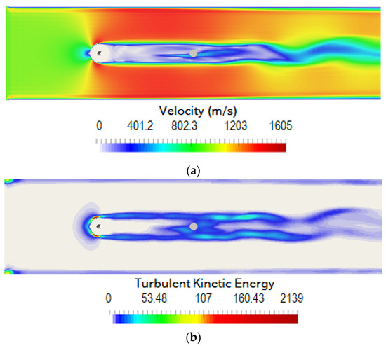
Figure 7. Steady-state flow features around the heated circular cylinder: (a) velocity-magnitude contour and (b) turbulent kinetic energy (TKE) distribution. The results highlight the formation of the wake region and the gradual decay of turbulence downstream.

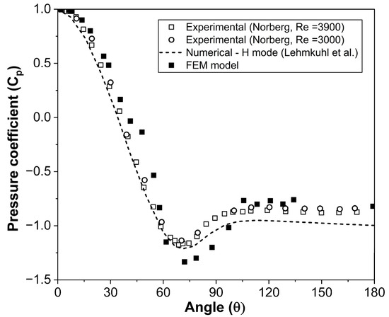
Figure 8. Comparison of the pressure coefficient distribution around a circular cylinder predicted by the present FEM model with experimental Laser Doppler Velocimetry data of Norberg (Re = 3000 and 3900) [40] and the numerical results of Lehmkuhl et al. [41].

In a subcritical flow, the laminar boundary layer separates at approximately 80° downstream of the front stagnation point, which agrees with the simulation in Figure 8, where vortex shedding is fully turbulent. In Norberg’s wind tunnel experiments [40] at Reynolds numbers between 3000 and 3900, surface pressure distributions were measured using pressure taps around the cylinder, clearly identifying the stagnation point, the suction peak near 70–80°, and the pressure recovery in the wake. The FEM model reproduces these features with good fidelity: the predicted pressure drop and separation angle are consistent with the experimental data. At the same time, the wake region shows the characteristic plateau associated with fully turbulent shedding. As illustrated in Figure 8, the H-mode data reported by Lehmkuhl et al. [41] capture the energetic state of the cylinder wake obtained from DNS at Re = 3900. Their study found that the flow oscillates slowly at a low frequency (f_m ≈ 0.0064), leading to the recirculation bubble alternating between contraction and expansion. This oscillation gives rise to two alternating flow states: a high-energy (H) mode characterized by more substantial shear-layer fluctuations and elevated turbulence levels, and a low-energy (L) mode characterized by weaker shear-layer fluctuations and a more extended wake. The H-mode corresponds to periods when the wake becomes more energetic and compact, driven by intensified shear-layer motion and enhanced base suction. Compared with the FEM results, the H-mode curve indicates slightly lower pressure recovery near the base, which suggests stronger entrainment and a shorter recirculation region during this energetic phase.

The instantaneous temperature plot in the domain is shown in Figure 9. The fluid temperature has decreased after the cylinder, while the cylinder’s temperature has increased dramatically due to the flow. However, the advection dominates as the temperature distribution ensues the fluid flow. Figure 9 shows the mean metal temperature along the x-axis at z = 5 cm and y = 2.5 cm (Figure 1). At x = −1.0, where the hot fluid first comes into contact with the cylinder surface, the metal temperature rises quickly from 373 K to nearly 600 K, reaching thermal equilibrium with the surrounding flow. Since the rear surface of the cylinder is minimally perturbed by the flow at 600 K, the temperature is lowest around the center between the two surfaces. Hence, at X = 1.0, the metal temperature was lower than that of the incoming fluid at x = −1.0 due to flow stagnation and a vortex behind the cylinder.

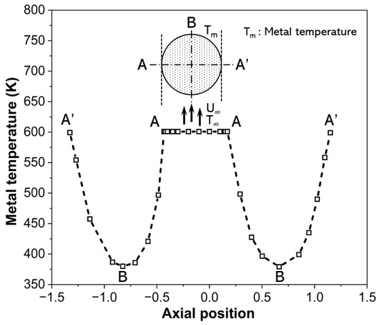
Figure 9. Temperature distribution along the x-axis at z = 5 cm and y = 2.5 cm, showing the metal cylinder temperature profile (T_m) and the surrounding fluid temperature field. The results illustrate the conjugate heat transfer between the solid cylinder and the flowing fluid, with a clear temperature gradient from the cylinder surface to the ambient flow.

Figure 10 illustrates the evolution of the wake behind the cylinder over time. The separatrices grow and shift with the shedding vortices and mark the regions where transport is organized and the flow is partitioned into distinct zones of coherent motion. The temperature field follows the vortices in the wake, showing that heat is carried downstream mainly by advection. New vortices are shed from the cylinder and attracting and repelling critical points appear in the wake. These points mark where structures form, grow stronger, and eventually decay. Saddle points highlight regions of strong stretching and folding, which are responsible for enhanced mixing of momentum and temperature. This combined view of the velocity skeleton and temperature contours provides a structural perspective on the wake: it captures not only the periodic shedding and growth of vortices but also the pathways through which turbulence transports thermal energy.

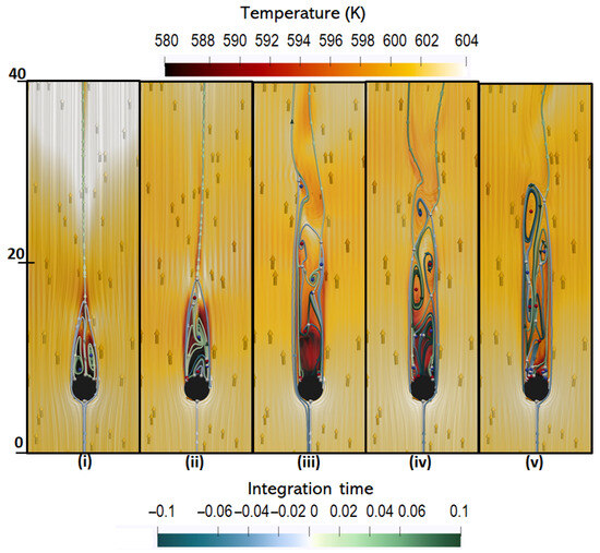
Figure 10. The transient profile of the topology along with the temperature contour on the YZ plane at (i) t = 0.0278, (ii) t = 0.0838, (iii) t = 0.1758, (iv) t = 0.34, and (v) t = 0.51. Critical points colored by type. Red: repelling, white: saddle, blue: attracting. The separatrices are colored by integration time starting at the corresponding saddle. The background visualizes the instantaneous velocity through Line Integral Convolution and the temperature through color coding.

The close alignment between topological boundaries and thermal features suggests that topology can serve as an effective diagnostic for identifying where heat and momentum exchange are most active. In this way, the analysis offers insights that go beyond scalar fields alone, linking vortex dynamics, turbulence propagation, and thermal transport into a coherent physical picture of the flow.

3.3. Case III: Spray Injection and Breakup Dynamics in Internal Combustion Engines

For the compressible flow case, the model was tested to study spracy injection and breakup dynamics against literature data from the engine combustion network [42]. The experimental operating conditions are reported by Sandia Spray G Data for different operating conditions, such as Spray G1, G2, G3, G2-cold, and G3 cold, etc, which are primarily categorized by different fuel types, fuel temperature, ambient temperature, ambient density, and absolute ambient pressure [43]. The model parameters include a cube size of 0.1 m³, an injector diameter of 0.00165 m, and standard operating conditions for the spray G1 presented in Table 2. Dirichlet boundary conditions were also applied. To assess mesh sensitivity, simulations were performed using 4 mm and 2 mm grids. The finer mesh yielded closer agreement with experimental penetration results, while the coarser grid showed reduced resolution, confirming that the formulation improves with refinement.

Table 2. ECN Spray G [42] operating condition (Case III).

Name	Tfuel [K]	Tair [K]	${\mathit{\rho }}_{\mathit{air}}$ [kg/m3]	Pa [kPa]	Pinj [MPa]	Electronic Injection [ms]	Fuel
G1 (Spray G standard)	363	573	3.5	600	20	0.68	Iso- octane

The dynamics of the injected spray in an internal combustion engine can be described in terms of the transition from a dense, coherent jet core to a dispersed droplet field [44]. As shown in Figure 11a, a schlieren image from the literature captures the early penetration of the liquid jet, highlighting the sharp inlet core that gradually loses coherence downstream. The experimental schlieren image from the literature provides direct evidence of the fundamental spray dynamics depicted schematically in Figure 11b. Close to the nozzle orifice, the spray emerges as a relatively coherent liquid core.

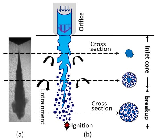
Figure 11. Spray injection in a compressible flow case: (a) representative schlieren image showing inlet core and breakup [45], (b) schematic highlighting entrainment and droplet distribution.

As the jet travels downstream, however, surface instabilities develop at the liquid–gas interface. These disturbances promote entrainment, which draws surrounding air into the spray and sets the stage for mixing and eventual breakup. This mixing enhances shear stresses and leads to wave growth on the jet surface and the onset of atomization. The breakup process itself progresses through multiple stages. Initially, large liquid ligaments detach from the unstable jet surface. These ligaments then undergo secondary breakup and fragment into smaller droplets under the combined influence of aerodynamic forces, surface tension, and turbulent eddies. The result is a non-homogeneous region with a wide distribution of droplet sizes, as indicated in the schematic cross sections. To assess the predictive capability of the proposed compressible flow scheme, the model was tested under a representative Spray G1 condition specified by the ECN. The liquid/vapor penetration and liquid volume fraction calculated from the model are compared against ECN experimental results in Figure 12 and Figure 13. Figure 12 compares experimental measurements (SNL ECN) with FEM predictions of liquid and vapor penetration under the Spray G1 condition. The penetration length is calculated based on the axial distribution of spray mass per unit length along the injector axis (z), which is positive in the direction of flow. An ensemble of spray droplets is sampled at discrete axial positions, and the corresponding droplet radii are used to calculate the variation in spray mass with distance from the injector tip.

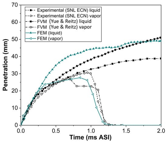
Figure 12. Comparison of the predicted and experimental liquid and vapor penetration lengths for the ECN Spray G1 case [42]. Results from the FEM model are compared with those from the finite volume method (FVM) models of Yue and Reitz using the same mesh resolution [46]. The FEM model captures both the temporal evolution and saturation behavior of the spray, showing close agreement with Sandia ECN experimental measurements for both the liquid and vapor phases.

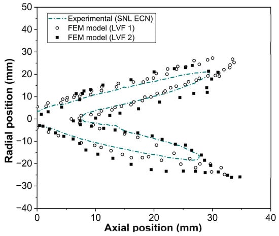
Figure 13. Comparison of the predicted and experimental radial spray profiles for the ECN Spray G1 case [42] at t = 0.8 ms. The FEM results agree well with the liquid and vapor phase penetration and radial dispersion for liquid volume fractions of 5 × 10⁻⁵ (LVF 1) and 0.001 (LVF 2).

The penetration length is then identified as the axial location where the local spray mass per unit length decreases below a specified fraction of the reference mass per unit length. For the experimental data, a threshold of 2 × 10⁻⁴ mass fraction was adopted to determine penetration length. The results suggest that the model captures the rapid initial increase and subsequent stabilization of liquid penetration at approximately 50 mm. Vapor penetration also follows the experimental trend, though discrepancies appear beyond 1 ms, which may be attributed to limitations in mesh resolution and evaporation modeling. In the present model, the flash-boiling evaporation formulation of Reitz and Price is applied [47,48,49], resulting in a pronounced reduction in liquid volume fraction downstream of 1.25 mm under an operating temperature of 573 K.

These comparisons demonstrate that the proposed compressible FEM framework reproduces the key features of liquid jet breakup and evaporation. For reference, the FEM results are also compared with the FVM results of Yue and Reitz [46] for the same mesh resolution of 2 mm. However, they exhibit slightly delayed saturation behavior due to differences in spatial discretization and phase change treatment. The statistical comparison between the FEM and FVM solvers highlights distinct differences in predictive performance and is presented in Table 3.

Table 3. Statistical Error Metrics for Liquid and Vapor Phases between FEM and FVM solvers.

Phase	Model	RMSE (mm)	NRMSE (-)	MAPE (%)	Mean Bias (mm)
Liquid	FEM	4.8496	0.1362	12.674	+3.5194
	FVM	6.9585	0.2003	26.023	−5.5637
Vapor	FEM	3.6214	0.2063	22.051	−0.6883
	FVM	3.6678	0.2164	22.442	−0.7314

The statistical comparison between the FEM and FVM solvers highlights distinct differences in predictive performance and is presented in Table 3. For the liquid phase, the FEM model demonstrated noticeably higher accuracy, with an RMSE (Root Mean Square Error) of 4.85 mm and a MAPE (Mean Absolute Percentage Error) of 12.7%, compared to 6.96 mm and 26.0% for the FVM model. This improvement reflects FEM’s improved accuracy in capturing sharp interfacial gradients and preserving solution smoothness without excessive numerical diffusion. The mean bias further indicates that the FEM solution slightly overpredicts the liquid thickness (+3.52 mm), whereas the FVM approach tends to underpredict (−5.56 mm), consistent with the diffusive nature of finite-volume discretization. The mean bias values further illustrate this contrast: the FEM model slightly overpredicts the liquid thickness (+3.52 mm), whereas the FVM model consistently underpredicts it (−5.56 mm), reflecting its more diffusive numerical nature. In contrast, the differences between the two solvers become much smaller in the vapor phase. Both methods yield comparable errors, with RMSE values of 3.62 mm (FEM) and 3.67 mm (FVM), and MAPE around 22%. The corresponding biases (−0.69 mm for FEM and −0.73 mm for FVM) suggest a mild underestimation but no significant systematic deviation. These results imply that the vapor region, characterized by weaker density gradients and smoother field variations, is less sensitive to the numerical formulation.

Figure 13 presents a comparison of experimental cut-plane data (SNL ECN) with model predictions for Spray G1 at t = 0.8 ms. The results are shown for two liquid volume fraction (LVF) thresholds: 5 × 10⁻⁵ and 1 × 10⁻³. The experimental profiles exhibit a near-symmetric radial spray distribution, with penetration increasing axially downstream of the nozzle. The FEM model (Figure 12 and Figure 13) can effectively capture both the axial penetration and radial spread of the spray plume across two different liquid volume fraction (LVF) thresholds. For the lower threshold (5 × 10⁻⁵), the predicted spray boundaries align well with the experimental envelope, showing that the model can reproduce the extent of the outer vapor–droplet mixing region. At the higher LVF threshold (0.001), the model continues to follow the experimental trend but slightly underpredicts the radial spread, particularly at larger axial distances. Such deviations are likely related to the mesh resolution, which affects the model’s ability to accurately represent detailed breakup and secondary atomization processes.

4. Conclusions

The objective of this study was to develop a unified VOF–FEM framework for simulating compressible multiphase flows with turbulence and conjugate heat transfer. The framework introduces a reconstruction-free interface approach, incorporates the dynamic Vreman LES model to represent subgrid-scale turbulence, and uses a weak-form finite-element formulation that ensures flux conservation without relying on prescribed heat transfer coefficients. The framework was implemented in both canonical and applied cases, which demonstrates the model’s broad applicability to spray combustion, thermal management, additive manufacturing, and high-speed aerospace flow systems. The dynamic Vreman LES model was used for its well-demonstrated robustness across compressible, transitional, and turbulent flow regimes. It adaptively adjusts the subgrid-scale dissipation based on local flow gradients, which eliminates the need for wall-damping functions. The predictive capability of the dynamic Vreman model in wall-bounded and shear-layer flows, as reported in prior studies [50,51], was also evident in the study, with accurate predictions of spray breakup in engine combustion. In the FEM framework, the interface between phases was captured directly without explicit geometric reconstruction. The weak-form FEM formulation with SUPG stabilization introduces controlled, flow-aligned regularization that suppresses interface oscillations while maintaining phase sharpness. This unified treatment allows the same numerical framework to handle both multiphase and conjugate heat transfer phenomena without introducing additional interface models. Because the fluid and solid domains share common nodes, thermal coupling emerges directly from the finite-element formulation rather than from imposed boundary conditions. This unified treatment of fluid–fluid and fluid–solid coupling highlights one of the key advantages of the FEM-based approach for complex multiphysics problems. To enhance the analysis beyond scalar flow and temperature fields, vector field topology was introduced to reveal the fundamental organization of vortices and instabilities. This method provided a systematic framework for visualizing flow organization, exposing critical points, separatrices, and coherent structures that are often overlooked by traditional scalar-field diagnostics.

The main advantage of the proposed FEM–VOF framework is its unified treatment of multiphase flow, turbulence, and conjugate heat transfer within a single weak-form formulation. This approach eliminates the need for separate interface-tracking or flux-balancing procedures and allows all coupled physics to be solved consistently within a single framework. Conversely, the model requires fewer numerical iterations and demonstrates higher computational efficiency than typical finite-volume or meshless methods at comparable spatio-temporal resolutions. A detailed quantitative error analysis confirmed this enhancement: the FEM model achieved an RMSE of 4.85 mm and MAPE of 12.7%, compared to 6.96 mm and 26.0% for the FVM model, highlighting the enhanced predictive capability of the proposed FEM approach in resolving interfacial dynamics. These results collectively demonstrate FEM’s robustness and accuracy in capturing interface motion and heat-transfer trends relative to benchmark and experimental data. While effective, the current formulation is still constrained by mesh resolution near steep interfaces, where limited numerical diffusion may affect fine-scale structures. Future work can explore adaptive meshing and higher-order interface representations to enhance accuracy and computational efficiency further. The framework can also be extended to incorporate compressibility and ionization effects, broadening its applicability to plasma–liquid interactions and other multiphysics systems where strong interfacial coupling governs transport and stability. Such extensions would enhance its relevance to low-temperature plasma modeling, spray combustion, and microfluidic applications.

References

- Xu, Y.; Subramaniam, S. Consistent modeling of interphase turbulent kinetic energy transfer in particle-laden turbulent flows. Phys. Fluids 2007, 19, 085101. [Google Scholar] [CrossRef]
- Han, Z.; Reitz, R.D. Turbulence Modeling of Internal Combustion Engines Using RNG κ-ε Models. Combust. Sci. Technol. 1995, 106, 267–295. [Google Scholar] [CrossRef]
- Pitsch, H.; Desjardins, O.; Balarac, G.; Ihme, M. Large-eddy simulation of turbulent reacting flows. Prog. Aerosp. Sci. 2008, 44, 466–478. [Google Scholar] [CrossRef][Green Version]
- Riley, J.J. Review of Large-Eddy Simulation of Non-Premixed Turbulent Combustion. J. Fluids Eng. 2004, 128, 209–215. [Google Scholar] [CrossRef]
- Duronio, F.; Ranieri, S.; Mascio, A.D.; Vita, A.D. Simulation of high pressure, direct injection processes of gaseous fuels by a density-based OpenFOAM solver. Phys. Fluids 2021, 33, 066104. [Google Scholar] [CrossRef]
- Mahamud, R.; Tropina, A.A.; Shneider, M.N.; Miles, R.B. Dual-pulse laser ignition model. Phys. Fluids 2018, 30, 106104. [Google Scholar] [CrossRef]
- Dettmer, W.; Perić, D. A computational framework for free surface fluid flows accounting for surface tension. Comput. Methods Appl. Mech. Eng. 2006, 195, 3038–3071. [Google Scholar] [CrossRef]
- Sirignano, W.A.; Mehring, C. Review of theory of distortion and disintegration of liquid streams. Prog. Energy Combust. Sci. 2000, 26, 609–655. [Google Scholar] [CrossRef]
- Christodoulou, K.N.; Scriven, L.E. Discretization of free surface flows and other moving boundary problems. J. Comput. Phys. 1992, 99, 39–55. [Google Scholar] [CrossRef]
- Rider, W.J.; Kothe, D.B. Reconstructing Volume Tracking. J. Comput. Phys. 1998, 141, 112–152. [Google Scholar] [CrossRef]
- Sussman, M.; Fatemi, E.; Smereka, P.; Osher, S. An improved level set method for incompressible two-phase flows. Comput. Fluids 1998, 27, 663–680. [Google Scholar] [CrossRef]
- Ling, Y.; Balachandar, S.; Parmar, M. Inter-phase heat transfer and energy coupling in turbulent dispersed multiphase flows. Phys. Fluids 2016, 28, 033304. [Google Scholar] [CrossRef]
- Hirt, C.W.; Nichols, B.D. Volume of fluid (VOF) method for the dynamics of free boundaries. J. Comput. Phys. 1981, 39, 201–225. [Google Scholar] [CrossRef]
- Theodorakakos, A.; Bergeles, G. Simulation of sharp gas–liquid interface using VOF method and adaptive grid local refinement around the interface. Int. J. Numer. Methods Fluids 2004, 45, 421–439. [Google Scholar] [CrossRef]
- Nichita, B.A.; Zun, I.; Thome, J.R. A Level Set Method Coupled with a Volume of Fluid Method for Modeling of Gas-Liquid Interface in Bubbly Flow. J. Fluids Eng. 2010, 132, 081302. [Google Scholar] [CrossRef]
- Kuerten, J.G.M.; van der Geld, C.W.M.; Geurts, B.J. Turbulence modification and heat transfer enhancement by inertial particles in turbulent channel flow. Phys. Fluids 2011, 23, 123301. [Google Scholar] [CrossRef]
- Waters, J.; Carrington, D.B.; Francois, M.M. Modeling multiphase flow: Spray breakup using volume of fluids in a dynamics LES FEM method. Numer. Heat Transf. Part B Fundam. 2017, 72, 285–299. [Google Scholar] [CrossRef]
- Yu, C.C.; Heinrich, J.C. Petrov-Galerkin methods for the time-dependent convective transport equation. Int. J. Numer. Methods Eng. 1986, 23, 883–901. [Google Scholar] [CrossRef]
- Carrington, D.B.; Ramos, O., Jr. FEARCE: Fast, Easy, Accurate, and Robust Continuum Engineering Improving Fuel Efficiency and Reducing Emissions in Combustion Engines 2019 R&D 100 Awards; Office of Scientific and Technical Information: Oak Ridge, TN, USA, 2019. [Google Scholar]
- Mirjalili, S.; Jain, S.S.; Dodd, M. Interface-capturing methods for two-phase flows: An overview and recent developments. Cent. Turbul. Res. Annu. Res. Briefs 2017, 2017, 13. [Google Scholar]
- Lyras, K.G.; Lee, J. A finite volume coupled level set and volume of fluid method with a mass conservation step for simulating two-phase flows. Int. J. Numer. Methods Fluids 2022, 94, 1027–1047. [Google Scholar] [CrossRef]
- Yan, S.-l.; Zhang, X.-b.; Luo, Z.-H. Adaptive mesh refinement for VOF modeling gas-liquid two-phase flow: A summary of some algorithms and applications. Chem. Eng. Sci. 2025, 306, 121291. [Google Scholar] [CrossRef]
- Milan, F.; Biferale, L.; Sbragaglia, M.; Toschi, F. Lattice Boltzmann simulations of droplet breakup in confined and time-dependent flows. Phys. Rev. Fluids 2020, 5, 033607. [Google Scholar] [CrossRef]
- Monteleone, A.; De Marchis, M.; Milici, B.; Napoli, E. A multi-domain approach for smoothed particle hydrodynamics simulations of highly complex flows. Comput. Methods Appl. Mech. Eng. 2018, 340, 956–977. [Google Scholar] [CrossRef]
- Ng, K.C.; Ng, Y.L.; Sheu, T.; Mukhtar, A. Fluid-solid conjugate heat transfer modelling using weakly compressible smoothed particle hydrodynamics. Int. J. Mech. Sci. 2019, 151, 772–784. [Google Scholar] [CrossRef]
- Salehi, F.; Beheshti, A.; Eftekharian, E.; Chen, L.; Hardalupas, Y. Data-driven modelling of spray flows: Current status and future direction. J. Energy Inst. 2025, 119, 101991. [Google Scholar] [CrossRef]
- Li, Y.; Zhao, C.; Cheng, S.; Guo, H. A data-driven phase change model for injection flow modeling. Phys. Fluids 2024, 36, 083324. [Google Scholar] [CrossRef]
- Mahamud, R.; Hasan, M.K.; Haque, M.A. Modeling of Turbulent Non-Premixed Combustion Using High Order Compact Finite Difference Method Combined with a Steady Flamelet Approach. In Proceedings of ASME International Mechanical Engineering Congress and Exposition, Portland, OR, USA, 17–21 November 2024. [Google Scholar]
- Haque, M.A.; Hasan, M.K.; Mahamud, R. A high-order compact finite difference scheme for flamelet-based scalar transport in non-premixed laminar flames. Phys. Fluids 2025, 37, 083637. [Google Scholar] [CrossRef]
- Laramee, R.S.; Hauser, H.; Zhao, L.; Post, F.H. Topology-Based Flow Visualization, The State of the Art. In Topology-Based Methods in Visualization; Springer: Berlin/Heidelberg, Germany, 2007; pp. 1–19. [Google Scholar]
- Bujack, R.; Yan, L.; Hotz, I.; Garth, C.; Wang, B. State of the Art in Time-Dependent Flow Topology: Interpreting Physical Meaningfulness Through Mathematical Properties. Comput. Graph. Forum 2020, 39, 811–835. [Google Scholar] [CrossRef]
- Waters, J.; Carrington, D.; Pepper, D.W. An Adaptive Finite Element Method with Dynamic LES for Turbulent Reactive Flows. Comput. Therm. Sci. Int. J. 2016, 8, 57–71. [Google Scholar] [CrossRef]
- Zienkiewicz, O.C.; Codina, R. A general algorithm for compressible and incompressible flow—Part I. the split, characteristic-based scheme. Int. J. Numer. Methods Fluids 1995, 20, 869–885. [Google Scholar] [CrossRef]
- Reitz, R. Modeling atomization processes in high-pressure vaporizing sprays. At. Spray Technol. 1987, 3, 309–337. [Google Scholar]
- O’Rourke, P.J.; Amsden, A. A Spray/Wall Interaction Submodel for the KIVA-3 Wall Film Model; SAE Transactions: Warrendale, PA, USA, 2000; pp. 281–298. [Google Scholar]
- Abramzon, B.; Sirignano, W.A. Droplet vaporization model for spray combustion calculations. Int. J. Heat Mass Transf. 1989, 32, 1605–1618. [Google Scholar] [CrossRef]
- Lilly, D. A proposed modification of the Germano subgrid-scale eddy viscosity model. Phys. Fluids A 1992, 4, 633–635. [Google Scholar] [CrossRef]
- Liu, W.; Wang, X.; Liu, X.; Yu, C.; Fang, M.; Ye, W. Pure single-mode Rayleigh-Taylor instability for arbitrary Atwood numbers. Sci. Rep. 2020, 10, 4201. [Google Scholar] [CrossRef] [PubMed]
- Tropina, A.A.; Mahamud, R. Effect of Plasma on the Deflagration to Detonation Transition. Combust. Sci. Technol. 2022, 194, 2752–2770. [Google Scholar] [CrossRef]
- Norberg, C. LDV-measurements in the near wake of a circular cylinder. In Proceedings of the ASME Fluids Engineering Division Summer Meeting, Washington, DC, USA, 21–25 June 1998. [Google Scholar]
- Lehmkuhl, O.; Rodríguez, I.; Borrell, R.; Oliva, A. Low-frequency unsteadiness in the vortex formation region of a circular cylinder. Phys. Fluids 2013, 25, 085109. [Google Scholar] [CrossRef]
- Hwang, J.; Weiss, L.; Karathanassis, I.K.; Koukouvinis, P.; Pickett, L.M.; Skeen, S.A. Spatio-temporal identification of plume dynamics by 3D computed tomography using engine combustion network spray G injector and various fuels. Fuel 2020, 280, 118359. [Google Scholar] [CrossRef]
- Abraham, J.; Pickett, L.M. Computed and measured fuel vapor distribution in a diesel spray. At. Sprays 2010, 20, 241–250. [Google Scholar] [CrossRef]
- Blume, M.; Schwarz, P.; Rusche, H.; Weiß, L.; Wensing, M.; Skoda, R. 3D Simulation of Turbulent and Cavitating Flow for the Analysis of Primary Breakup Mechanisms in Realistic Diesel Injection Processes. At. Sprays 2019, 29, 861–893. [Google Scholar] [CrossRef]
- El Marnissi, Y.; Hwang, J. Microscopic imaging on diesel spray and atomization process. Processes 2024, 12, 359. [Google Scholar] [CrossRef]
- Yue, Z.; Reitz, R.D. Application of an equilibrium-phase spray model to multicomponent gasoline direct injection. Energy Fuels 2019, 33, 3565–3575. [Google Scholar] [CrossRef]
- Reitz, R.D. A photographic study of flash-boiling atomization. Aerosol Sci. Technol. 1990, 12, 561–569. [Google Scholar] [CrossRef]
- Price, C.; Hamzehloo, A.; Aleiferis, P.; Richardson, D. Aspects of Numerical Modelling of Flash-Boiling Fuel Sprays; 0148-7191; SAE Technical Paper: Warrendale, PA, USA, 2015. [Google Scholar]
- Adachi, M.; McDonell, V.G.; Tanaka, D.; Senda, J.; Fujimoto, H. Characterization of Fuel Vapor Concentration Inside a Flash Boiling Spray; 0148-7191; SAE Technical Paper: Warrendale, PA, USA, 1997. [Google Scholar]
- Vreman, B.; Geurts, B.; Kuerten, H. On the formulation of the dynamic mixed subgrid-scale model. Phys. Fluids 1994, 6, 4057–4059. [Google Scholar] [CrossRef]
- You, D.; Moin, P. A dynamic global-coefficient subgrid-scale eddy-viscosity model for large-eddy simulation in complex geometries. Phys. Fluids 2007, 19, 065110. [Google Scholar] [CrossRef]
Disclaimer/Publisher’s Note: The statements, opinions and data contained in all publications are solely those of the individual author(s) and contributor(s) and not of MDPI and/or the editor(s). MDPI and/or the editor(s) disclaim responsibility for any injury to people or property resulting from any ideas, methods, instructions or products referred to in the content. |
© 2025 by the authors. Licensee MDPI, Basel, Switzerland. This article is an open access article distributed under the terms and conditions of the Creative Commons Attribution (CC BY) license (https://creativecommons.org/licenses/by/4.0/).