
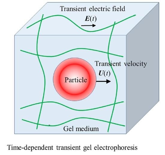
Transient Gel Electrophoresis of a Spherical Colloidal Particle

Abstract
1. Introduction
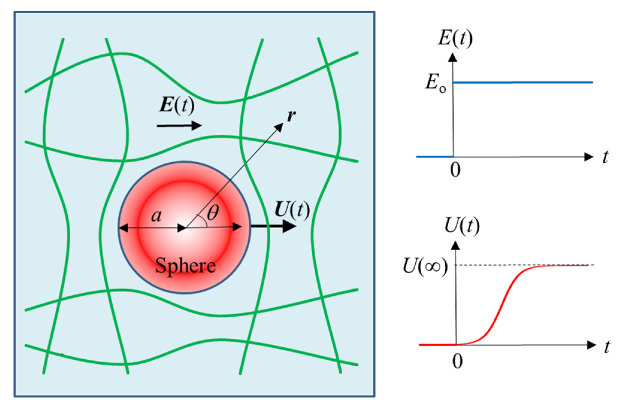
2. Theory
2.1. Fundamental Electrokinetic Equations
2.2. Weak Electric Field Approximation
2.3. General Expression for the Laplace Transform of the Transient Gel Electrophoretic Mobility
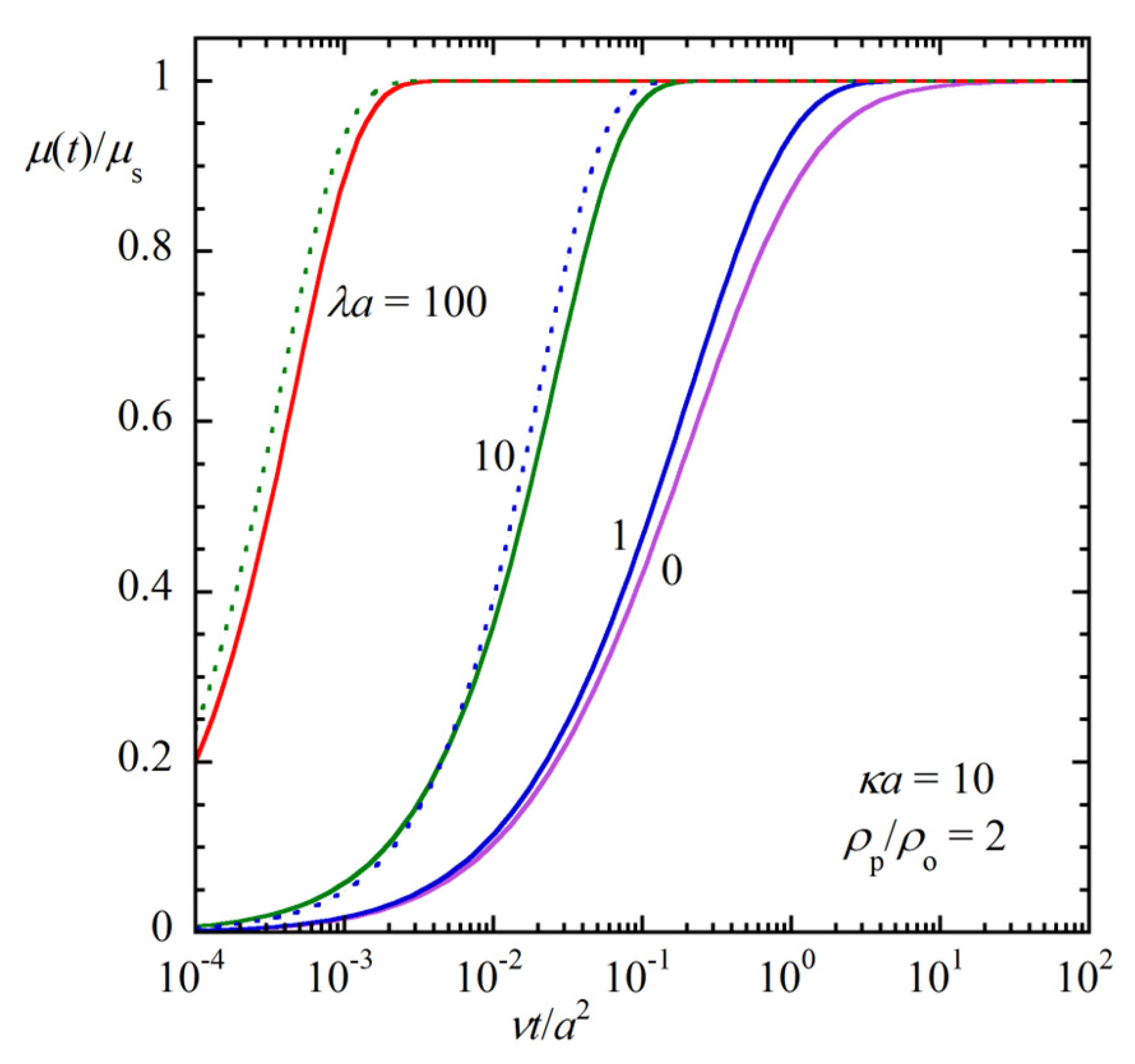
3. Results and Discussion
4. Conclusions
Funding
Institutional Review Board Statement
Informed Consent Statement
Data Availability Statement
Conflicts of Interest
References
- Morrison, F.A. Transient electrophoresis of a dielectric sphere. J. Colloid Interface Sci. 1969, 29, 687–691. [Google Scholar] [CrossRef]
- Morrison, F.A. Transient electrophoresis of an arbitrarily oriented cylinder. J. Colloid Interface Sci. 1971, 36, 139–145. [Google Scholar] [CrossRef]
- Ivory, C.F. Transient electroosmosis: The momentum transfer coefficient. J. Colloid Interface Sci. 1983, 96, 296–298. [Google Scholar] [CrossRef]
- Ivory, C.F. Transient electroosmosis of a dielectric sphere. J. Colloid Interface Sci. 1984, 100, 239–249. [Google Scholar] [CrossRef]
- Keh, H.J.; Tseng, H.C. Transient electrokinetic flow in fine capillaries. J. Colloid Interface Sci. 2001, 242, 450–459. [Google Scholar] [CrossRef]
- Keh, H.J.; Huang, Y.C. Transient electrophoresis of dielectric spheres. J. Colloid Interface Sci. 2005, 291, 282–291. [Google Scholar] [CrossRef] [PubMed]
- Huang, Y.C.; Keh, H.J. Transient electrophoresis of spherical particles at low potential and arbitrary double-layer thickness. Langmuir 2005, 21, 11659–11665. [Google Scholar] [CrossRef]
- Khair, A.S. Transient phoretic migration of a permselective colloidal particle. J. Colloid Interface Sci. 2012, 381, 183–188. [Google Scholar] [CrossRef] [PubMed]
- Chiang, C.C.; Keh, H.J. Startup of electrophoresis in a suspension of colloidal spheres. Electrophoresis 2015, 36, 3002–3008. [Google Scholar] [CrossRef]
- Chiang, C.C.; Keh, H.J. Transient electroosmosis in the transverse direction of a fibrous porous medium. Colloids Surf. A Physicochem. Engin. Asp. 2015, 481, 577–582. [Google Scholar] [CrossRef]
- Li, M.X.; Keh, H.J. Start-up electrophoresis of a cylindrical particle with arbitrary double layer thickness. J. Phys. Chem. B 2020, 124, 9967–9973. [Google Scholar] [CrossRef]
- Lai, Y.C.; Keh, H.J. Transient electrophoresis of a charged porous particle. Electrophoresis 2020, 41, 259–265. [Google Scholar] [CrossRef]
- Lai, Y.C.; Keh, H.J. Transient electrophoresis in a suspension of charged particles with arbitrary electric double layers. Electrophoresis 2021, 42, 2126–2133. [Google Scholar] [CrossRef]
- Ohshima, H. Approximate analytic expression for the time-dependent transient electrophoretic mobility of a spherical colloidal particle. Molecules 2022, 27, 5108. [Google Scholar] [CrossRef] [PubMed]
- Ohshima, H. Transient electrophoresis of a spherical soft particle. Colloid Polym. Sci. 2022, 300, 1369–1377. [Google Scholar] [CrossRef]
- Ohshima, H. Transient electrophoresis of a cylindrical colloidal particle. Fluids 2022, 7, 342. [Google Scholar] [CrossRef]
- Ohshima, H. Transient electrophoresis of a spherical colloidal particle with a slip surface. Electrophoresis 2023. [Google Scholar] [CrossRef] [PubMed]
- Stigter, D. Influence of agarose gel on electrophoretic stretch, on trapping, and on relaxation of DNA. Macromolecules 2000, 33, 8878–8889. [Google Scholar] [CrossRef]
- Allison, S.A.; Xin, Y.; Pei, H. Electrophoresis of spheres with uniform zeta potential in a gel modeled as an effective medium. J. Colloid Interface Sci. 2007, 313, 328–337. [Google Scholar] [CrossRef]
- Hanauer, M.; Pierrat, S.; Zins, I.; Lotz, A.; Sönnichsen, C. Separation of nanoparticles by gel electrophoresis according to size and shape. Nano Lett. 2007, 7, 2881–2885. [Google Scholar] [CrossRef]
- Allison, S.A.; Pei, H.; Xin, Y. Review modeling the free solution and gel electrophoresis of biopolymers: The bead array-effective medium model. Biopolymers 2007, 87, 102–114. [Google Scholar] [CrossRef]
- Mohammadi, M.; Hill, R.J. Steady electrical and micro-rheological response functions for uncharged colloidal inclusions in polyelectrolyte hydrogels. Proc. R. Soc. A 2010, 466, 213–235. [Google Scholar] [CrossRef]
- Hsu, J.P.; Huang, C.H.; Tseng, S. Gel electrophoresis: Importance of concentration-dependent permittivity and double-layer polarization. Chem. Eng. Sci. 2012, 84, 574–579. [Google Scholar] [CrossRef]
- Hsu, J.P.; Huang, C.H.; Tseng, S. Gel electrophoresis of a charge-regulated, bi-functional particle. Electrophoresis 2013, 34, 785–791. [Google Scholar] [CrossRef] [PubMed]
- Li, F.; Hill, R.J. Nanoparticle gel electrophoresis: Bare charged spheres in polyelectrolyte hydrogels. J. Colloid Interface Sci. 2013, 394, 1–12. [Google Scholar] [CrossRef]
- Li, F.; Allison, S.A.; Hill, R.J. Nanoparticle gel electrophoresis: Soft spheres in polyelectrolyte hydrogels under the Debye-Hückel approximation. J. Colloid Interface Sci. 2014, 423, 129–142. [Google Scholar] [CrossRef]
- Allison, S.A.; Li, F.; Hill, R.J. The electrophoretic mobility of a weakly charged “soft”sphere in a charged hydrogel: Application of the Lorentz reciprocal theorem. J. Phys. Chem. B 2014, 118, 8827–8838. [Google Scholar] [CrossRef] [PubMed]
- Bhattacharyya, S.; De, A.; Gopmandal, P.P. Electrophoresis of a colloidal particle embedded in electrolyte saturated porous media. Chem. Eng. Sci. 2014, 118, 184–191. [Google Scholar] [CrossRef]
- Allison, S.A.; Li, F.; Le, M. Electrophoretic mobility of a dilute, highly charged “soft” spherical particle in a charged hydrogel. J. Phys. Chem. B 2016, 120, 8071–8079. [Google Scholar] [CrossRef]
- Hill, R.J. Electrokinetics of nanoparticle gel-electrophoresis. Soft Matter 2016, 12, 8030–8048. [Google Scholar] [CrossRef]
- Bhattacharyya, S.; De, S. Gel electrophoresis and size selectivity of charged colloidal particles in a charged hydrogel medium. Chem. Eng. Sci. 2016, 141, 304–314. [Google Scholar] [CrossRef]
- Bhattacharyya, S.; De, S. Nonlinear effects on electrophoresis of a charged dielectric nanoparticle in a charged hydrogel medium. Phys. Fluids 2016, 28, 092006. [Google Scholar] [CrossRef]
- Le, L. Numerical Calculation of Gel Electrophoretic Mobility for “Soft” Spherical Nanoparticle. Master’s Thesis, McGill University, Montreal, QC, Canada, 2017. [Google Scholar]
- Majee, P.S.; Bhattacharyya, S.; Gopmandal, P.P.; Ohshima, H. On gel electrophoresis of dielectric charged particles with hydrophobic surface: A combined theoretical and numerical study. Electrophoresis 2018, 39, 794–806. [Google Scholar] [CrossRef] [PubMed]
- Ohshima, H. Electrophoretic mobility of a charged spherical colloidal particle in an uncharged or charged polymer gel medium. Colloid Polym. Sci. 2019, 297, 719–728. [Google Scholar] [CrossRef]
- Ohshima, H. Gel electrophoresis of a soft particle. Adv. Colloid Interface Sci. 2019, 271, 101977. [Google Scholar] [CrossRef] [PubMed]
- Barman, S.S.; Bhattacharyya, S.; Gopmandal, P.P.; Ohshima, H. Impact of charged polarizable core on mobility of a soft particle embedded in a hydrogel medium. Colloid Polym. Sci. 2020, 298, 1729–1739. [Google Scholar] [CrossRef]
- Ohshima, H. Electrophoretic mobility of a soft particle in a polymer gel medium. Colloids Surf. A Physicochem. Eng. Asp. 2021, 618, 126400. [Google Scholar] [CrossRef]
- Bharti; Sarkar, S.; Ohshima, H.; Gopmandal, P.P. Gel electrophoresis of a hydrophobic liquid droplet with an equipotential slip surface. Langmuir 2022, 38, 8943–8953. [Google Scholar] [CrossRef]
- Saad, E.J.; Faltas, M.S. Time-dependent electrophoresis of a dielectric spherical particle embedded in Brinkman medium. Z. Angew. Math. Phys. 2018, 69, 43. [Google Scholar] [CrossRef]
- Saad, E.J. Start-up Brinkman electrophoresis of a dielectric sphere for Happel and Kuwabara models. Math Meth. Appl. Sci. 2018, 41, 9578–9591. [Google Scholar] [CrossRef]
- Saad, E.J. Unsteady electrophoresis of a dielectric cylindrical particle suspended in porous medium. J. Mol. Liquid 2019, 289, 111050. [Google Scholar] [CrossRef]
- Sherief, H.H.; Faltas, M.S.; Ragab, K.E. Transient electrophoresis of a conducting spherical particle embedded in an electrolyte-saturated Brinkman medium. Electrophoresis 2021, 42, 1636–1647. [Google Scholar] [CrossRef]
- Brinkman, H.C. A calculation of the viscous force exerted by a flowing fluid on a dense swarm of particles. Appl. Sci. Res. 1947, 1, 27–34. [Google Scholar] [CrossRef]
- Debye, P.; Bueche, A.M. Intrinsic viscosity, diffusion, and sedimentation rate of polymers in solution. J. Chem. Phys. 1948, 16, 573–579. [Google Scholar] [CrossRef]
- O’Brien, R.W.; White, L.R. Electrophoretic mobility of a spherical colloidal particle. J. Chem. Soc. Faraday Trans. 2 Mol. Chem. Phys. 1978, 74, 1607–1626. [Google Scholar] [CrossRef]


Disclaimer/Publisher’s Note: The statements, opinions and data contained in all publications are solely those of the individual author(s) and contributor(s) and not of MDPI and/or the editor(s). MDPI and/or the editor(s) disclaim responsibility for any injury to people or property resulting from any ideas, methods, instructions or products referred to in the content. |
© 2023 by the author. Licensee MDPI, Basel, Switzerland. This article is an open access article distributed under the terms and conditions of the Creative Commons Attribution (CC BY) license (https://creativecommons.org/licenses/by/4.0/).
Share and Cite
Ohshima, H. Transient Gel Electrophoresis of a Spherical Colloidal Particle. Gels 2023, 9, 356. https://doi.org/10.3390/gels9050356
Ohshima H. Transient Gel Electrophoresis of a Spherical Colloidal Particle. Gels. 2023; 9(5):356. https://doi.org/10.3390/gels9050356
Chicago/Turabian StyleOhshima, Hiroyuki. 2023. "Transient Gel Electrophoresis of a Spherical Colloidal Particle" Gels 9, no. 5: 356. https://doi.org/10.3390/gels9050356
APA StyleOhshima, H. (2023). Transient Gel Electrophoresis of a Spherical Colloidal Particle. Gels, 9(5), 356. https://doi.org/10.3390/gels9050356