Simple Summary
Methane (CH4) produced from rumen fermentation in cattle is a major agricultural source of greenhouse gas (GHG) emissions that contributes to global warming. Therefore, accurate prediction of CH4 production from this process is critical for developing national CH4 emission inventories and evaluating dietary strategies to mitigate GHG emissions. Based on the in vitro fermentation of CH4 production, this study established a large-scale experimental database, which included training set data and test set data, respectively. Prediction models for CH4 production in vitro were developed by using multiple linear regression (MLR) analysis and backpropagation neural network (BPNN) technique, with the carbohydrate (Carbs) components of the Cornell Net Carbohydrate and Protein System (CNCPS) in the mixed rations as the input variable. The root mean square prediction error (RMSPE), coefficient of determination (r2), and concordance correlation coefficient (CCC) of the MLR and the BPNN prediction models were evaluated and compared using the test set data. In conclusion, compared with the MLR model (RMSPE% = 3.42%, r2 = 0.91, CCC = 0.92), the BPNN model (RMSPE% = 2.29%, r2 = 0.93, CCC = 0.96) is more accurate in predicting the CH4 production during rumen fermentation.
Abstract
Methane (CH4) produced by methanogenic archaea during the rumen fermentation of feed carbohydrates leads to global warming and total energy loss. This study aims to compare the accuracy of multiple linear regression (MLR) models and backpropagation neural network (BPNN) in predicting ruminal CH4 production of the carbohydrate (Carbs) components of the Cornell Net Carbohydrate and Protein System (CNCPS) in mixed rations of beef cattle with different concentrate-to-forage (C/F) ratios. Two datasets were established using the in vitro fermentation method of Menke and Steingass. One of the datasets contained 60 mixed rations with C/F ratios of 30:70, 40:60, 50:50, 60:40, 70:30, 80:20, and 90:10, respectively, which were used to develop CH4 prediction models. Another dataset included 10 mixed rations with the same C/F ratios, which were used to validate and compare the accuracy of the prediction models. Results indicated that there was a significant multiple regression relationship between CH4 production and the Carbs-components (CA (sugars), CB1 (starch and pectin), CB2 (available cell wall), CC (unavailable cell wall)) of CNCPS (r2 = 0.91, p < 0.0001). An optimal BPNN model with 2 hidden-layer neuron nodes was established with the same variables (r2 = 0.93, p < 0.0001). The findings demonstrated that both MLR and BPNN models (p < 0.0001) were suitable for predicting CH4 production using the Carbs components (CA, CB1, CB2, CC) of CNCPS. However, compared with the MLR model, the BPNN model has a greater coefficient of determination (r2) value and concordance correlation coefficient (CCC), and a lower root mean square prediction error (RMSPE), demonstrating better prediction performance.
1. Introduction
Methane (CH4) is an important greenhouse gas (GHG), with a 100-year warming potential 28 times that of carbon dioxide (CO2), contributing significantly to global climate change [1]. A total of 159 countries, along with the European Commission, have committed to the Global Methane Pledge, which aims to reduce anthropogenic CH4 emissions by at least 30% by the year 2030, relative to levels recorded in 2020 [2]. This initiative seeks to achieve the goal of limiting the increase in global temperatures to no more than 1.5 °C [3]. Agriculture contributes 40% of CH4 emissions resulting from human activities, making it the primary source of this potent and environmentally detrimental GHG. Approximately 80% of agricultural CH4 emissions are generated from enteric fermentation in ruminants [4]. It is worth noting that beef and dairy production systems contribute over 70% of livestock GHG emissions [5].
The importance of mitigating CH4 emission has been increasingly recognized, highlighting the urgent need for precise quantitative techniques to formulate effective strategies for mitigating climate change [6]. However, due to the limitations of measurement techniques and high costs, it is difficult to assess enteric CH4 emissions in a commercial setting [7]. To enhance the accuracy of predicting enteric CH4 emissions in cattle, numerous prediction models have been reported, including univariate linear regression models [8,9], multiple linear regression (MLR) models [8,10,11], nonlinear models [12], and dynamic mechanistic models [13,14]. These models investigate the factors influencing CH4 production by examining the underlying mechanisms of CH4 formation in rumen fermentation. They incorporate key variables such as dry matter intake (DMI) [8,9], gross energy intake (GEI) [9], and metabolizable energy intake (MEI) [8], neutral detergent fiber intake (NDFI) [8,11], acid detergent fiber intake (ADFI) [8,11], ether extract (EE) [10], and forage proportion [8], which can be utilized as predictors for estimating CH4 output. However, application of the empirical models [7] beyond the range of the data used for model development can result in errors in CH4 prediction [15]. The predictive performance of CH4 models improves with massive datasets for model development. Many studies have shown that CH4 production during rumen fermentation is related to the dietary carbohydrates consumed by cattle [16]. In the Cornell Net Carbohydrate and Protein system (CNCPS), the carbohydrate (Carbs) components are divided into four components of CA (sugars), CB1 (starch and pectin), CB2 (available cell wall), and CC (unavailable cell wall), based on the rate of degradation in the rumen [17]. Dong et al. [18] indicated that the Carbs-components of the CNCPS in mixed rations were closely correlated with CH4 production in rumen fermentation; however, the mixed rations in that study are limited to low concentrate-to-forage (C/F) ratios. The C:F ratios in feeds affects CH4 production in ruminants by shifting rumen fermentation patterns and proportions of volatile fatty acids (VFAs) [19].
The artificial neural network (ANN) offers a powerful alternative for predicting CH4 emissions in ruminants. ANNs capture the complexity of the rumen microbial fermentation system through its capacity for nonlinear mapping and self-learning [20]. Unlike traditional statistical models, ANNs effectively characterize nonlinear relationships between input variables and CH4 emissions without requiring a predetermined functional form [21]. Furthermore, ANNs demonstrate significant advantages when managing high-dimensional datasets [22]. Shadpour et al. [23] predicted CH4 emissions from dairy cattle through the application of multilayer perceptron neural networks. Their findings highlight the ability of ANN to identify intricate patterns in milk composition that are linked to CH4 emissions. Sahraei et al. [24] evaluated Long Short-Term Memory networks, which had an R2 of 0.88 and a mean bias error (MBE) of 13.55 ppm CH4, demonstrating promising potential for predicting CH4 emissions in dairy cows. It can be presumed that using ANN algorithms to develop models can optimize the CH4 prediction in ruminants from diet compositions.
The objective of the present study was to investigate the relationship between CH4 production and the Carbs-components of the CNCPS in mixed rations of beef cattle with a wide range of C/F ratios. Additionally, an artificial neural network model based on backpropagation was developed using the CNCPS Carbs-components as input variables to determine whether the accuracy of the CH4 prediction models could be further improved.
2. Materials and Methods
This study comprises the following components: (1) Dataset construction: Two datasets were constructed for model development. (2) Variable selection: The CNCPS Carbs -components of various mixed rations were selected as independent variables of the model, with in vitro CH4 production as the dependent variable. (3) Model development: Two modeling approaches of a multiple linear regression (MLR) model and a backpropagation neural network (BPNN) were developed. (4) Model evaluation: The predictive performance of the developed models was validated and compared.
2.1. Construction of Two Datasets
Two independent datasets were constructed for modeling and validation. The modeling dataset used for simulation training included 60 mixed rations with C/F ratios of 30:70, 40:60, 50:50, 60:40, 70:30, 80:20, and 90:10, respectively (Table 1). The validation dataset was used to evaluate model performance, comprising 10 mixed rations with the same C/F ratios (Table 2). These dietary formulations were designed based on the ingredient compositions and C/F ratios commonly used in typical feeding practices for beef cattle in China [18].

Table 1.
Typical mixed rations for beef cattle used to establish models with concentrate-to-forage ratios (C/F) ranging from low to high (%, dry matter basis).
Table 2.
Typical mixed rations for beef cattle used to validate models with concentrate-to-forage ratios (C/F) ranging from low to high (%, dry matter basis).
2.2. In Vitro Fermentation
The in vitro CH4 production of mixed rations was determined by the in vitro fermentation method of Menke and Steingass [25]. Four Simmental bulls fitted with permanent rumen fistulas (Anscitech Co., Ltd., Wuhan, China) were used as donors of rumen fluid. The daily ration for the cattle consisted of 24.0 kg WCS and 4.0 kg concentrate mixture (as-fed basis). The concentrate was composed of 60% corn, 18% soybean meal, 13% wheat bran, 2% calcium hydrogen phosphate, 1% sodium chloride, 1% sodium bicarbonate, and 5% trace element mixture. The management of the cattle was conducted according to the Laboratory Animal Ethics Committee of the College of Animal Science and Technology at Qingdao Agricultural University (Approval No. DKY20240420). Two hours before the morning feeding, 100 mL of rumen fluid was collected from each cattle via rumen fistulas. The rumen fluid of the four bulls was thoroughly mixed and quickly filtered through four layers of gauze into a warmed bottle maintained at 39 °C. The filtered rumen fluid was mixed with artificial buffered saliva [25] in a ratio of 1:2 to prepare the rumen fluid–buffer mixture. The 100 mL calibrated glass syringes were used as the fermentation vessels. Each syringe was filled with 0.2000 g of the mixed ration, and the syringes were prewarmed to 39 °C before use. Four syringes were designated as replicates for each mixed ration within each experimental run. A total of three independent fermentation runs were conducted. Each fermentation syringe was loaded with 30 mL of 1:2 rumen fluid–buffer mixture. The syringes were flushed with CO2 to remove air, and the heads of the syringes were sealed. The syringes were then incubated on a rotary shaker platform in a water bath maintained at 39 °C for 48 h. The cumulative gas production of the mixed ration was recorded, and the pH of the fermentation broth was determined using a digital pH meter after 48 h of fermentation. After 48 h of incubation, a 20 mL gas sample was collected through a three-way plug valve between the sampling syringe and the incubation syringe to determine the gas concentration. The CH4 concentrations in the gas samples were analyzed by gas chromatography (TP-2060T, Beijing Beifen Tianpu Instrument Technology Co., Ltd., Beijing, China). The chromatographic conditions, including the TCD detector, carrier gas, and standard gas composition, were consistent with those previously described by Dong and Zhao [18]. The analysis was conducted using the following conditions: a TCD detector and a TDX-01 column (dimensions 1 m × 2 mm × 3 mm) were used, with the column maintained at 70 °C and the detector at 100 °C. Argon was used as the carrier gas at a flow rate of 30 mL/min. The standard gas included 26.796% CH4, 65.300% CO2, 0.605% O2, 7.100% N2, and 0.199% H2 (v/v).
2.3. Chemical Analysis of the Mixed Ration
The chemical composition of dry matter (DM), ether extract (EE), CP, and ash contents of the feed samples were analyzed using method 930.15, 984.13, 920.39 and 942.05 of AOAC [26]. Starch content was determined as described by Dong and Zhao [18] with an enzyme kit containing thermostable α-amylase and amyloglucosidase (Megazyme International Ireland Ltd., Wicklow, Ireland). The neutral detergent fiber (NDF) content (method 2002.04) was determined using the ANKOM fiber system (ANKOM Technology, Macedon, NY, USA). Neutral detergent insoluble crude protein (NDICP) was quantified as the crude protein content in the residues following NDF analysis. During the determination process, heat-stable α-amylase (ANKOM Technology) and sodium sulfite (ANKOM Technology) were used. The acid detergent lignin contents were determined using method 973.18 of AOAC [26].
2.4. Calculations
The CNCPS Carbs-components CA (sugars), CB1 (starch and pectin), CB2 (available cell wall), and CC (unavailable cell wall) of the mixed rations were determined using the method of Sniffen et al. [17], and presented in Table 3 and Table 4, respectively.
where NSC refers to non-structural carbohydrate, and NDICP is neutral detergent insoluble crude protein.
CA [%DM] = NSC [%DM] − Starch [%DM]
CB1 [%DM] = Starch [%DM]
CB2 [%DM] = NDF [%DM] − NDICP [%DM] − CC [%DM]
CC [%DM] = Lignin [%DM] × 2.4
NSC [%DM] = 100 − CP [%DM] − Ash [%DM] − EE [%DM] − CB2 [%DM] − CC [%DM]
Table 3.
The CNCPS components (% DM) of typical rations for beef cattle used to develop models.
Table 4.
The CNCPS components (%DM) of typical rations for beef cattle used to validate models.
CH4 concentration from the syringe was corrected for blanks and expressed as the amount of substrate dry matter (mL CH4/g DM). The CH4 production was calculated using the equation as follows:
where refers to CH4 production of mixed rations after 48 h, and is CH4 production of the blank after 48 h of incubation.
2.5. Construction of MLR Prediction Models
The Carbs-components CA (sugars), CB1 (starch and pectin), CB2 (available cell wall), and CC (unavailable cell wall) of CNCPS of the dataset containing 60 mixed rations were used as independent variables for model input, and the in vitro CH4 production corresponding to 60 mixed rations was used as dependent variable for model output. The multiple regression relationship between the in vitro CH4 production (mL/g DM) and Carbs-components (%DM) of CNCPS was investigated using the following equation:
where y refers to in vitro CH4 or CO2 production; bis the constant; and , , and are coefficients.
2.6. Construction of BPNN Prediction Models
A three-layer backpropagation neural network (BPNN) architecture including input layer neurons, hidden layer neurons, and output layer neurons was used in this study [27]. The input layer neurons are composed of four variables, CA, CB1, CB2 and CC. The hidden layer structure is a single monolayer with a different number of neurons. The output layer neuron contains an output variable for in vitro CH4 or CO2 production.
The BPNN model was developed on the MATLAB R2024a platform (The Math Works, Natick, MA, USA, 2024) using in vitro CH4 or CO2 production and CNCPS Carbs-components, which were derived from a training dataset containing 60 mixed rations. The training parameters included a learning rate of 0.1, training epochs of 1000, and a performance goal of 0.00001. The codes were runed in MATLAB R2024a as follows:
- >>
- Independent variable_train = Independent variable_train’;
- >>
- Dependent variable_train = Dependent variable_train’;
- >>
- Independent variable_validation = Independent variable_validation’;
- >>
- net = newff (Independent variable_train, Dependent variable_train, hidden layer number);
- >>
- net.trainParam.epochs = 1000;
- >>
- net.trainParam.lr = 0.1;
- >>
- net.trainParam.goal = 0.00001;
- >>
- net = train(net, Independent variable_train, Dependent variable_train);
- >>
- Predicted Dependent variable_validation = sim(net, Independent variable_validaton);
- >>
- Predicted Dependent variable_validation
The prediction performance of BPNN architectures with 1 to 20 neurons in the hidden layer was evaluated using the validation dataset.
2.7. Comparison of the Predictive Performance of MLR and BPNN
The validation dataset included in vitro CH4 or CO2 production and the CNCPS Carbs-components of 10 other mixed rations for evaluating the MLR models and BPNN models. The performance of the model was evaluated using the following four methods:
A t-test was used to compare the observed and the predicted values;
A linear regression relationship between the observed and the predicted values was analyzed using the following equation:
where x and y refer to the observed and predicted values, mL/g DM of mixed rations.
The root mean square prediction error (MSPE) [28] was calculated to quantify the deviation between the observed and the predicted values:
where i = 1, 2, …, n; refers to the observed value; , the predicted value; and n, the number of determinations. RMSPE is the ratio of the observed mean used to indicate the overall prediction error, %;
The concordance correlation coefficient (CCC) was calculated according to the formula reported by Lin [29].
2.8. Statistical Analysis
Statistical analysis was performed using SAS version 9.4 (SAS Institute Inc., Cary, NC, USA). Multiple linear regression (MLR) relationships between the dependent and independent variables were analyzed by using the PROC MIXED procedure. Selection of independent variables for the CH4 prediction equation was based on stepwise regression analysis, and only those with statistical significance (p ≤ 0.05) were retained. The assessment of multicollinearity among independent variables was conducted using the “vif” function, with the tolerance level set at a variance inflation factor <5.0. The t-test was used to compare the observed and predicted values, and the PROC MIXED procedure was used to analyze the linear relationship between them.
3. Results
3.1. The CH4 and CO2 Productions Through In Vitro Fermentation
The in vitro CH4 production for the 60 mixed rations with varying concentrate-to-forage ratios used for model development was presented in Table 5. After 48 h in vitro fermentation, the pH values of the fermentation residues were within the range of 6.10 to 6.80, indicating normal in vitro ruminal fermentation.
Table 5.
The CH4, CO2 productions (mL/g DM), and pH values of typical rations for beef cattle used to develop models.
3.2. The Multiple Regression Relationship Between CH4 Emissions and CNCPS C-Components
The significant multiple regression equation between ruminal CH4 production in vitro and the Carbs-components CA (sugars), CB1 (starch and pectin), CB2 (available cell wall), and CC (unavailable cell wall) of the CNCPS was as follows:
CH4 (mL/g DM) = (0.22 ± 0.08) CA + (0.32 ± 0.05) CB1 − (0.13 ± 0.05) CB2 − (0.49 ± 0.09) CC + (34.05 ± 4.20)
(R2 = 0.85, n = 60, p < 0.0001, MLR model)
(R2 = 0.85, n = 60, p < 0.0001, MLR model)
The significant multiple regression equation between ruminal CO2 production in vitro and the Carbs-components CA, CB1, CB2, and CC of the CNCPS was as follows:
CO2 (mL/g DM) = (2.34 ± 0.34) CA + (3.27 ± 0.24) CB1 + (0.44 ± 0.23) CB2 − (1.75 ± 0.41) CC + (36.35 ± 18.27)
(R2 = 0.93, n = 60, p < 0.0001, MLR model)
(R2 = 0.93, n = 60, p < 0.0001, MLR model)
3.3. The BPNN Model
After 1000 training epochs, the target error of 0.00001 was achieved. The RMSPE% of the BPNN model in predicting in vitro CH4 and CO2 production, with the number of hidden layer neuron nodes ranging from 1 to 20, is shown in Table 6. When the number of neuron nodes in the hidden layer was 2 and 15, respectively, the RMSPE% values for predicting the in vitro CH4 and CO2 production were the lowest. Therefore, the BPNN architectures suitable for predicting the in vitro CH4 and CO2 production were identified as 4-2-1 (Figure 1) and 4-15-1 (Figure 2), respectively. The BPNN models for predicting in vitro CH4 and CO2 production are presented in Figure 3.
Table 6.
RMSPE% and r2 values between observed and predicted values across different hidden layer nodes.
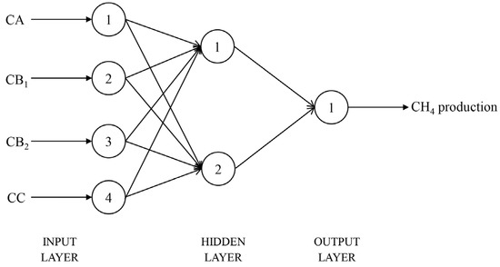
Figure 1.
Structural diagram of the BPNN model for CH4 production prediction (CA = sugars, CB1 = starch and pectin, CB2 = available cell wall, CC = unavailable cell wall).
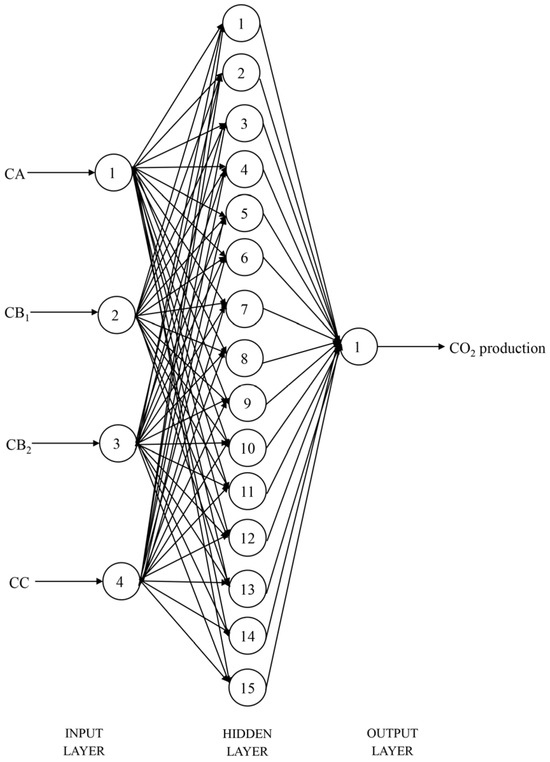
Figure 2.
Structural diagram of the backpropagation neural network model for CO2 production prediction (CA = sugars, CB1 = starch and pectin, CB2 = available cell wall, CC = unavailable cell wall).
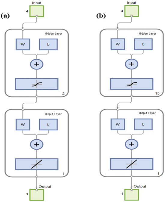
Figure 3.
Backpropagation neural network models for (a) CH4 production and (b) CO2 production running on MATLAB.
3.4. Comparative Validation of the MLR and BPNN Models
The t-test results indicated that there was no statistically significant difference between the observed and predicted in vitro CH4 production for either the MLR (p = 0.14, Table 7) or the BPNN model (p = 0.76, Table 7). There was a significant linear regression relationship between the observed in vitro CH4 production and the predicted in vitro CH4 production based on the MLR (r2 = 0.91, p < 0.0001, n = 10; Figure 4a) and the BPNN model (r2 = 0.93, p < 0.0001, n = 10; Figure 4b). The RMSPE% and CCC values of the MLR and BPNN models were 3.42% vs. 2.29% and 0.92 vs. 0.96, respectively.
Table 7.
The CH4, CO2 productions (mL/g DM), and pH values of typical rations for beef cattle used to validate models.
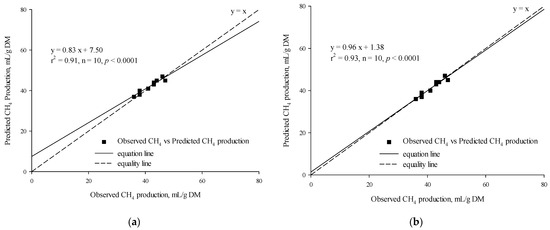
Figure 4.
Linear relationship between the observed vs. the predicted (a) CH4 production from the multiple linear regression model and (b) CH4 production from the backpropagation neural network model.
The t-test results revealed no statistically significant difference between the observed and predicted in vitro CO2 production for either the MLR model (p = 0.68) or the BPNN model (p = 0.31). A strong linear regression relationship was found between the observed in vitro CO2 production and the predicted in vitro CO2 production using the MLR model (r2 = 0.96, p = 0.0046, n = 10; Figure 5a) and the BPNN model (r2 = 0.98, p = 0.0046, n = 10; Figure 5b). The RMSPE% values of the MLR and BPNN models were 4.13% and 2.95%, while their CCC values were 0.97 and 0.99, respectively.
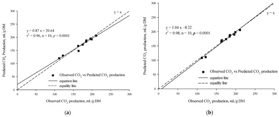
Figure 5.
Linear relationship between the observed vs. the predicted (a) CO2 production from the multiple linear regression model and (b) CO2 production from the backpropagation neural network model.
4. Discussion
Since in vitro gas production is closely related to enteric CH4 yield in vitro (r = 0.88), the in vitro rumen fermentation technique can be used as a dynamic estimation tool to predict enteric CH4 emissions in vitro [30]. In addition, measuring enteric CH4 emissions through the in vitro rumen fermentation method can facilitate the development of a large dataset essential for accurate CH4 prediction models. A pH range of 6.0 to 6.8 is optimal for maintaining the stability of the rumen’s internal conditions [31]. In this study, the pH value of the incubation residues fell within the normal range. Furthermore, rumen microorganisms were found to remain active after the in vitro fermentation, indicating that the in vitro incubation system was effectively functioning.
The carbohydrate components of ruminant feeds in the CNCPS reflect the fermentation degradability in rumen [17]. In the current study, there was a significant multiple regression relationship between the CNCPS-Carbs components in mixed rations with varying C/F ratios and the in vitro CH4 production, with an R2 of 0.85. This regression determination coefficient is consistent with the multiple regression equation reported by Wang et al. [11]. The results demonstrated that the CA, CB1, CB2, and CC four components in CNCPS are suitable variables for predicting CH4 production of mixed rations with different C/F ratios. In addition, the coefficients of CA, CB1, and CB2 in the MLR prediction model were 0.22, 0.32, and 0.13 mL/g DM, respectively, demonstrating that CB2 had a lower CH4 production compared with CA and CB1. This finding is consistent with the previous work of Dong et al. (2013) [18]. Selecting the appropriate predictor variables could enhance the model’s prediction effect on CH4 production. A linear mixed model established by Oikawa et al. [32] that included DMI, BW, and milk fat as predictors had an R2 of 0.66 and a CCC of 0.66. One possible reason for the low accuracy of that study might be that the dataset is limited to typical feed ingredients from Japan. Vargas et al. [33] evaluated the predictive performance of 72 models for predicting CH4 emissions in beef cattle, and found that the RMSPE value of the Ellis et al. [8] model (including the prediction variables of DMI and EE) was as low as 17.79%, and the CCC value was 0.21. The MLR model established in this study could be used in cattle production to identify low CH4 emitting feed formulas [34]. By manipulating the proportions of CNCPS components, producers can pre-emptively design rations that not only meet the nutritional requirements of animals but also reduce CH4 emissions.
In recent years, researchers have applied deep learning methods to develop prediction models to enhance the accuracy of CH4 prediction [35]. The enteric CH4 produced from rumen fermentation of ruminants is a complex and dynamic reaction process [36]. The ANN algorithms provide advanced tools for dynamically simulating complex relational models [37]. Most studies apply ANNs to predict parameters in various fields to help further improve the accuracy of the model development. Jassim et al. [38] developed a multi-layer perceptron artificial neural network to predict municipal solid waste generation, with an R2 value of 0.94. Odufuwa et al. [39] evaluated emissions of pollutants such as CO2 and nitrogen oxides (NOx). The ANN model demonstrated outstanding accuracy, with a regression (R) value exceeding 0.9 and a mean square error (MSE) as low as 0.0046 under a multiple training-validation-test configuration. Louime et al. [40] designed a convolutional Neural Network (CNN) model to accurately predict CH4 emissions from seaweed. In this study, BPNN was used to develop the CH4 production model and demonstrated superior predictive performance (r2 = 0.94). Sahraei et al. [24] developed a deep learning model that used a moderate and public dataset to predict CH4 productions from enteric fermentation in dairy cows, substantially improving the model performance (R2 = 0.74). There may be a nonlinear relationship between CH4 emissions and production traits, as Shadpour et al. [23] found that compared with linear ANNs and partial least squares (PLS) regression, nonlinear artificial neural networks (ANNs) had better predictive performance. In this study, the BPNN models are developed based on a nonlinear function of the Levenberg–Marquardt algorithm. Each neuron in the input layer is connected to the neurons of the hidden layer and then linked to the output layer through connection weighs [41]. Therefore, the number of neuron nodes in the hidden layer may affect the learning efficiency of the neural network and subsequently influence the prediction performance of the model. In this study, a different number of neurons in the hidden layer ranging from 1 to 20 were trained in the BPNN models, and the RMSPE showed some fluctuations with different neuron nodes. The results indicated that the BPNN with two hidden layer nodes can reduce CH4 emissions by 2.12%, which has great potential in the real-time application of dynamic rumen microbial fermentation. This indicates that ≥3 neurons in the hidden layer will lead to overfitting of the neural network, while only 1 neuron in the hidden layer will result in insufficient training of the neural network. It should be noted that the limitation of this study lies in the relatively small sample size of the validation dataset (n = 10). In future research, its predictive performance still needs to be further tested in larger databases.
The accuracy of BPNN and MLR models in predicting enteric CH4 and CO2 productions in vitro was compared using the validation dataset of this study. It revealed that the r2 and CCC values of the BPNN model were greater than those of the MLR model, while the RMSPE value was lower than that of the MLR model. The results show that when the four CNCPS Carbs-components were available, the BPNN approach outperforms the MLR model, demonstrating the potential of artificial intelligence in predicting enteric CH4 emissions in cattle. This finding is consistent with the predicted ruminal ammonia-N [27], indicating that the ANN algorithm has superior overall performance in predicting rumen fermentation parameters. Similarly, Stamenković et al. [42] demonstrated that the predictive performance of the ANN model was much better than that of the conventional MLR model when predicting CH4 emission in 20 European countries. Previous studies have reported that the ANN model performed better than the random forest (RF) model [43], and the performance of BPNN is better than that of the nonlinear regression models [44]. It is reported that the machine learning method (R2 ≥ 0.61) outperforms the linear method (R2 ≤ 0.56) in predicting CH4 production from anaerobic digestion of lignocellulosic biomass [45]. Due to its powerful nonlinear capabilities and inherent self-learning characteristics of complex systems, ANN models have become important tools for predicting enteric CH4 emissions of ruminants [46]. Compared with traditional empirical regression models, neural networks can effectively capture the complex relationships between input variables and CH4 emissions without the need to predefine the functional forms. It lays the foundation for incorporating ANN technique into future sustainable environmental strategies and promotes the development of carbon reduction technologies. In addition to its predictive ability, the BPNN model for predicting CH4 productions established in this study has significant potential in biological applications. As a computer simulator, it can accelerate pre-screen the CH4 mitigation potential of dietary interventions before conducting costly in vivo trials. In addition, this model offers a new approach for precise feeding of ruminants, allowing for the formulation of dietary strategies based on predicted CH4 emission phenotypes. In the future, additional research is necessary to integrate the microbial community, genotypes, and production data to develop highly robust models for accurately estimating enteric CH4 emissions from cattle [47].
5. Conclusions
There is a significant multiple linear regression relationship between the enteric CH4 production in vitro and the CNCPS Carbs-components (CA, CB1, CB2, and CC) within varying C/F ratios of mixed rations. The BPNN model can accurately simulate the intrinsic relationship between the carbohydrate composition of feed and CH4 production during ruminal anaerobic fermentation. The r2 and CCC values are relatively large, while the RMSPE value is relatively low. This method provides an artificial predictive tool for cattle farming, enabling pre-emptive diet design that not only meets the nutritional requirements of animals but also reduces CH4 emissions.
Author Contributions
Conceptualization, R.D.; methodology, G.Y. and Z.L.; validation, G.Y.; formal analysis, G.Y. and R.D.; investigation, Z.L.; resources, G.Y.; data curation, G.Y. and Z.L.; writing—original draft preparation, G.Y.; writing—review and editing, R.D.; visualization, G.Y. and Z.L.; supervision, R.D.; project administration, R.D.; funding acquisition, R.D. All authors have read and agreed to the published version of the manuscript.
Funding
This study was funded by the National Natural Science Foundation of China (grant number 32202691), the Natural Science Foundation of Shandong Province (grant number ZR2022QC027), and the Key R&D Program of Shandong Province, China (2024TZXD024).
Institutional Review Board Statement
The animal study protocol was approved by the Laboratory Animal Ethics Committee of the College of Animal Science and Technology at Qingdao Agricultural University (protocol code DKY20240420) on 20 April 2024.
Informed Consent Statement
Not applicable.
Data Availability Statement
The original contributions presented in this study are included in the article. Further inquiries can be directed to the corresponding author.
Conflicts of Interest
The authors declare no conflicts of interest.
References
- IPCC. Climate Change 2014: Synthesis Report. Contribution of Working Groups I, II and III to the Fifth Assessment Report of the Intergovernmental Panel on Climate Change; Pachauri, R.K., Meyer, L.A., Eds.; IPCC: Geneva, Switzerland, 2014; p. 151. [Google Scholar]
- Predybaylo, E.; Lelieveld, J.; Pozzer, A.; Gromov, S.; Zimmermann, P.; Osipov, S.; Klingmüller, K.; Steil, B.; Stenchikov, G.; McCabe, M. Surface temperature and ozone responses to the 2030 Global Methane Pledge. Clim. Change 2025, 178, 78. [Google Scholar] [CrossRef]
- IPCC. Summary for Policymakers. In Global Warming of 1.5 °C; Masson-Delmotte, V., Zhai, P., Pörtner, H.-O., Roberts, D., Skea, J., Shukla, P.R., Pirani, A., Moufouma-Okia, W., Péan, C., Pidcock, R., Eds.; Cambridge University Press: Cambridge, UK; New York, NY, USA, 2018; pp. 3–24. [Google Scholar]
- CCAC. Global Methane Assessment: Benefits and Costs of Mitigating Methane Emissions; United Nations Climate and Clean Air Coalition: Paris, France, 2021; Available online: https://www.ccacoalition.org/resources/global-methane-assessment-full-report (accessed on 1 May 2025).
- Gerber, P.J.; Steinfeld, H.; Henderson, B.; Mottet, A.; Opio, C.; Dijkman, J.; Falcucci, A.; Tempio, G. Tackling Climate Change Through Livestock: A Global Assessment of Emissions and Mitigation Opportunities; Food and Agriculture Organization of the United Nations (FAO): Rome, Italy, 2013. [Google Scholar]
- Beauchemin, K.A.; Kebreab, E.; Cain, M.; VandeHaar, M.J. The path to net-zero in dairy production: Are pronounced decreases in enteric methane achievable? Annu. Rev. Anim. Biosci. 2025, 13, 325–341. [Google Scholar] [CrossRef]
- Hristov, A.N.; Ott, T.; Tricarico, J.; Rotz, A.; Waghorn, G.; Adesogan, A.; Dijkstra, J.; Montes, F.; Oh, J.; Kebreab, E. Special topics—Mitigation of methane and nitrous oxide emissions from animal operations: III. A review of animal management mitigation options. J. Anim. Sci. 2013, 91, 5095–5113. [Google Scholar] [CrossRef]
- Ellis, J.; Kebreab, E.; Odongo, N.; McBride, B.; Okine, E.; France, J. Prediction of methane production from dairy and beef cattle. J. Dairy Sci. 2007, 90, 3456–3466. [Google Scholar] [CrossRef]
- Ribeiro, R.; Rodrigues, J.; Maurício, R.; Borges, A.; e Silva, R.R.; Berchielli, T.; Valadares Filho, S.; Machado, F.; Campos, M.; Ferreira, A. Predicting enteric methane production from cattle in the tropics. Animal 2020, 14, s438–s452. [Google Scholar] [CrossRef] [PubMed]
- Donadia, A.B.; Torres, R.N.S.; Silva, H.M.d.; Soares, S.R.; Hoshide, A.K.; Oliveira, A.S.d. Factors affecting enteric emission methane and predictive models for dairy cows. Animals 2023, 13, 1857. [Google Scholar] [CrossRef]
- Wang, Y.; Song, W.; Wang, Q.; Yang, F.; Yan, Z. Predicting enteric methane emissions from dairy and beef cattle using nutrient composition and intake variables. Animals 2024, 14, 3452. [Google Scholar] [CrossRef] [PubMed]
- Patra, A.K. Prediction of enteric methane emission from cattle using linear and non-linear statistical models in tropical production systems. Mitig. Adapt. Strateg. Glob. Change 2017, 22, 629–650. [Google Scholar] [CrossRef]
- Kass, M.; Ramin, M.; Hanigan, M.; Huhtanen, P. Comparison of Molly and Karoline models to predict methane production in growing and dairy cattle. J. Dairy Sci. 2022, 105, 3049–3063. [Google Scholar] [CrossRef]
- Muñoz-Tamayo, R.; Ruiz, B.; Blavy, P.; Giger-Reverdin, S.; Sauvant, D.; Williams, S.; Moate, P. Predicting the dynamics of enteric methane emissions based on intake kinetic patterns in dairy cows fed diets containing either wheat or corn. Animal 2022, 1, 100003. [Google Scholar] [CrossRef]
- Escobar-Bahamondes, P.; Oba, M.; Beauchemin, K. Universally applicable methane prediction equations for beef cattle fed high-or low-forage diets. Can. J. Anim. Sci. 2016, 97, 83–94. [Google Scholar] [CrossRef]
- Xue, B.; Thompson, J.P.; Yan, T.; Stergiadis, S.; Smith, L.; Theodoridou, K. Dose–response effects of dietary inclusion of agro-industrial by-products on in vitro ruminal fermentation and methane production. J. Sci. Food Agric. 2025, 105, 5447–5457. [Google Scholar] [CrossRef]
- Sniffen, C.J.; O’connor, J.; Van Soest, P.J.; Fox, D.G.; Russell, J. A net carbohydrate and protein system for evaluating cattle diets: II. Carbohydrate and protein availability. J. Anim. Sci. 1992, 70, 3562–3577. [Google Scholar] [CrossRef]
- Dong, R.; Zhao, G. Relationship between the methane production and the CNCPS carbohydrate fractions of rations with various concentrate/roughage ratios evaluated using in vitro incubation technique. Asian-Australas J. Anim. Sci. 2013, 26, 1708. [Google Scholar] [CrossRef][Green Version]
- Fouts, J.Q.; Honan, M.C.; Roque, B.M.; Tricarico, J.M.; Kebreab, E. Enteric methane mitigation interventions. Transl. Anim. Sci. 2022, 6, txac041. [Google Scholar] [CrossRef]
- Li, R.; Xu, A.; Zhao, Y.; Chang, H.; Li, X.; Lin, G. Genetic algorithm (GA)—Artificial neural network (ANN) modeling for the emission rates of toxic volatile organic compounds (VOCs) emitted from landfill working surface. J. Environ. Manag. 2022, 305, 114433. [Google Scholar] [CrossRef]
- Liu, X.; Tao, F.; Du, H.; Yu, W.; Xu, K. Learning nonlinear constitutive laws using neural network models based on indirectly measurable data. J. Appl. Mech. 2020, 87, 081003. [Google Scholar] [CrossRef]
- Castillo-Girones, S.; Munera, S.; Martínez-Sober, M.; Blasco, J.; Cubero, S.; Gómez-Sanchis, J. Artificial neural networks in agriculture, the core of artificial intelligence: What, when, and why. Comput. Electron. Agric. 2025, 230, 109938. [Google Scholar] [CrossRef]
- Shadpour, S.; Chud, T.C.; Hailemariam, D.; Plastow, G.; Oliveira, H.R.; Stothard, P.; Lassen, J.; Miglior, F.; Baes, C.F.; Tulpan, D. Predicting methane emission in Canadian Holstein dairy cattle using milk mid-infrared reflectance spectroscopy and other commonly available predictors via artificial neural networks. J. Dairy Sci. 2022, 105, 8272–8285. [Google Scholar] [CrossRef]
- Sahraei, A.; Knob, D.; Lambertz, C.; Gattinger, A.; Breuer, L. Modeling enteric methane emission from dairy cows using deep learning approach. Sci. Total Environ. 2025, 984, 179713. [Google Scholar] [CrossRef] [PubMed]
- Menke, K.H.; Steingass, H. Estimation of the energetic feed value obtained from chemical analysis and in vitro gas production using rumen fluid. Anim. Res. Dev. 1988, 28, 7–55. Available online: https://ci.nii.ac.jp/naid/10025840911/ (accessed on 1 April 2024).
- Association of Official Analytical Chemists (AOAC). Official Methods of Analysis, 18th ed.; AOAC International: Gaithersburg, MD, USA, 2005. [Google Scholar]
- Dong, R.; Sun, G.; Yu, G. Estimating in vitro ruminal ammonia-N using multiple linear models and artificial neural networks based on the CNCPS nitrogenous fractions of cattle rations with low concentrate/roughage ratios. J. Anim. Physiol. Anim. Nutr. 2022, 106, 841–853. [Google Scholar] [CrossRef]
- Bibby, J.; Toutenburg, H. Prediction and Improved Estimation in Linear Models; Wiley: Chichester, UK, 1977; p. 188. [Google Scholar]
- Lin, L.I. A concordance correlation coefficient to evaluate reproducibility. Biometrics 1989, 45, 255–268. [Google Scholar] [CrossRef]
- Aboagye, I.A.; Rosser, C.L.; Baron, V.S.; Beauchemin, K.A. In vitro assessment of enteric methane emission potential of whole-plant barley, oat, triticale and wheat. Animals 2021, 11, 450. [Google Scholar] [CrossRef] [PubMed]
- Liang, J.; Fang, W.; Chang, J.; Zhang, G.; Ma, W.; Nabi, M.; Zubair, M.; Zhang, R.; Chen, L.; Huang, J. Long-term rumen microorganism fermentation of corn stover in vitro for volatile fatty acid production. Bioresour. Technol. 2022, 358, 127447. [Google Scholar] [CrossRef] [PubMed]
- Oikawa, K.; Terada, F.; Kurihara, M.; Suzuki, T.; Nonaka, I.; Hosoda, K.; Kamiya, Y.; Roh, S.; Haga, S. Methane emission prediction models for lactating cows based on feed intake, body weight, and milk yield and composition: Variable methane conversion factor-based approach. J. Dairy Sci. 2025, 108, 7248–7261. [Google Scholar] [CrossRef] [PubMed]
- Vargas, J.; Swenson, M.; Schilling-Hazlett, A.; Reis, I.; Velasquez, C.; Martins, E.; Sitorski, L.; Campos, L.; Carvalho, P.; Stackhouse-Lawson, K. Evaluation of models of enteric methane emissions in finishing steers. Animal 2025, 19, 101536. [Google Scholar] [CrossRef]
- Williams, S.R.O.; Hannah, M.C.; Jacobs, J.L.; Wales, W.J.; Moate, P.J. Volatile fatty acids in ruminal fluid can be used to predict methane yield of dairy cows. Animals 2019, 9, 1006. [Google Scholar] [CrossRef]
- Alcibahy, M.; Gafoor, F.A.; Mustafa, F.; El Fadel, M.; Al Hashemi, H.; Al Hammadi, A.; Al Shehhi, M.R. Improved estimation of carbon dioxide and methane using machine learning with satellite observations over the Arabian Peninsula. Sci. Rep. 2025, 15, 766. [Google Scholar] [CrossRef]
- Vivares, G.; Dijkstra, J.; Bannink, A. Modeling diurnal rumen metabolism dynamics in dairy cattle: An update to a mechanistic model representing eating behavior, rumen content, rumination, and acid-base balance. J. Dairy Sci. 2025, 108, 6934–6957. [Google Scholar] [CrossRef]
- Legaard, C.; Schranz, T.; Schweiger, G.; Drgoňa, J.; Falay, B.; Gomes, C.; Iosifidis, A.; Abkar, M.; Larsen, P. Constructing neural network based models for simulating dynamical systems. ACM Comput. Surv. 2023, 55, 236. [Google Scholar] [CrossRef]
- Jassim, M.S.; Coskuner, G.; Zontul, M. Comparative performance analysis of support vector regression and artificial neural network for prediction of municipal solid waste generation. Waste Manag. Res. 2022, 40, 195–204. [Google Scholar] [CrossRef]
- Odufuwa, O.; Tartibu, L.; Kusakana, K. Artificial neural network modelling for predicting efficiency and emissions in mini-diesel engines: Key performance indicators and environmental impact analysis. Fuel 2025, 387, 134294. [Google Scholar] [CrossRef]
- Louime, C.J.; Raza, T.A. Development of artificial intelligence/machine learning (AI/ML) models for methane emissions forecasting in seaweed. Methane 2024, 3, 485–499. [Google Scholar] [CrossRef]
- Bukhari, M.M.; Alkhamees, B.F.; Hussain, S.; Gumaei, A.; Assiri, A.; Ullah, S.S. An improved artificial neural network model for effective diabetes prediction. Complexity 2021, 2021, 5525271. [Google Scholar] [CrossRef]
- Stamenković, L.J.; Antanasijević, D.; Ristić, M.; Perić-Grujić, A.; Pocajt, V. Modeling of methane emissions using the artificial neural network approach. J. Serb. Chem. Soc. 2015, 80, 421–433. [Google Scholar] [CrossRef]
- Liu, J.; Huang, Q.; Ulishney, C.; Dumitrescu, C.E. Comparison of random forest and neural network in modeling the performance and emissions of a natural gas spark ignition engine. J. Energy Resour. Technol. 2022, 144, 032310. [Google Scholar] [CrossRef]
- Suraboyina, S.; Allu, S.K.; Anupoju, G.R.; Polumati, A. A comparative predictive analysis of back-propagation artificial neural networks and non-linear regression models in forecasting seasonal ozone concentrations. J. Earth Syst. Sci. 2022, 131, 189. [Google Scholar] [CrossRef]
- Wang, Z.; Peng, X.; Xia, A.; Shah, A.A.; Yan, H.; Huang, Y.; Zhu, X.; Zhu, X.; Liao, Q. Comparison of machine learning methods for predicting the methane production from anaerobic digestion of lignocellulosic biomass. Energy 2023, 263, 125883. [Google Scholar] [CrossRef]
- Wu, Y.-C.; Feng, J.-W. Development and application of artificial neural network. Wirel. Pers. Commun. 2018, 102, 1645–1656. [Google Scholar] [CrossRef]
- Negussie, E.; González-Recio, O.; Battagin, M.; Bayat, A.R.; Boland, T.; de Haas, Y.; Garcia-Rodriguez, A.; Garnsworthy, P.C.; Gengler, N.; Kreuzer, M.; et al. Integrating heterogeneous across-country data for proxy-based random forest prediction of enteric methane in dairy cattle. J. Dairy Sci. 2022, 105, 5124–5140. [Google Scholar] [CrossRef] [PubMed]
Disclaimer/Publisher’s Note: The statements, opinions and data contained in all publications are solely those of the individual author(s) and contributor(s) and not of MDPI and/or the editor(s). MDPI and/or the editor(s) disclaim responsibility for any injury to people or property resulting from any ideas, methods, instructions or products referred to in the content. |
© 2025 by the authors. Licensee MDPI, Basel, Switzerland. This article is an open access article distributed under the terms and conditions of the Creative Commons Attribution (CC BY) license (https://creativecommons.org/licenses/by/4.0/).