Article

Are Source Code Metrics “Good Enough” in Predicting Security Vulnerabilities? †

Department of Computer Science and Media Technology, Linnaeus University, 351 95 Växjö, Sweden
*
Authors to whom correspondence should be addressed.
This paper is an extended version of our paper published in Ninth Swedish Workshop on Data Science (SweDS21), Växjö, Sweden, 2–3 December 2021.
Data 2022, 7(9), 127; https://doi.org/10.3390/data7090127
Submission received: 15 July 2022 / Revised: 10 August 2022 / Accepted: 22 August 2022 / Published: 7 September 2022

Abstract

:
Modern systems produce and handle a large volume of sensitive enterprise data. Therefore, security vulnerabilities in the software systems must be identified and resolved early to prevent security breaches and failures. Predicting security vulnerabilities is an alternative to identifying them as developers write code. In this study, we studied the ability of several machine learning algorithms to predict security vulnerabilities. We created two datasets containing security vulnerability information from two open-source systems: (1) Apache Tomcat (versions 4.x and five 2.5.x minor versions). We also computed source code metrics for these versions of both systems. We examined four classifiers, including Naive Bayes, Decision Tree, XGBoost Classifier, and Logistic Regression, to show their ability to predict security vulnerabilities. Moreover, an ensemble learner was introduced using a stacking classifier to see whether the prediction performance could be improved. We performed cross-version and cross-project predictions to assess the effectiveness of the best-performing model. Our results showed that the XGBoost classifier performed best compared to other learners, i.e., with an average accuracy of 97% in both datasets. The stacking classifier performed with an average accuracy of 92% in Struts and 71% in Tomcat. Our best-performing model—XGBoost—could predict with an average accuracy of 87% in Tomcat and 99% in Struts in a cross-version setup.

1. Introduction

Security vulnerability identification is essential to implementing and operating secured software systems. As such, the security of a system is also subject to the quality of its underlying source code. Poor code quality may make the system vulnerable to third-party access, i.e., introduce security threats. A previous study showed that an attack on the Equifax system exposed 143 million user accounts, for which the open-source nature of the Apache Struts system was at fault [1].
Previously, identification and prevention of security vulnerabilities or software bugs were performed using manual reviews, which today is impossible for systems with a large codebase. Thus, automatic code inspection tools (e.g., JSLint [2] or SonarQube [3]) were developed to identify vulnerabilities in software based on known code patterns or structures. However, the challenge of automatically identifying security vulnerabilities as early as possible in the software development lifecycle remains. In the literature, various software testing methods for identifying vulnerabilities, e.g., fuzztesting or fuzzing, are shown to be useful, however, at the later steps of the software development lifecycle [4].
NordVPN reported that without security patches installed, attackers may exploit vulnerabilities [5]. This study aimed to assist developers and security analysts by identifying security vulnerabilities in software systems. To do similarly, we have studied security vulnerabilities in two systems: a Jakarta servlet engine (Apache Tomcat, Forest Hill, MD, USA) and an MVC framework for creating elegant, modern Java web applications (Apache Struts, Forest Hill, MD, USA). We chose Apache Tomcat and Struts2-core because they are open-source systems with publicly available security logs.
The presence of security vulnerabilities in a system significantly increases the cost of quality assurance. In particular, modern large systems have a large volume of codebase, which makes it hard and time-consuming for developers to trace security vulnerabilities in the source code. Security vulnerabilities in a system usually go unmarked until the system is delivered and deployed. Therefore, in this study, intending to help developers and security analysts, we construct several machine learning (ML) models to predict security vulnerabilities in the source code, relying on static source code metrics that are easy to gather from the source code. We rely on publicly available vulnerability information to build two vulnerability datasets.
In this study, we answer the following four research questions:
  • RQ1: How do the individual learners perform while predicting the security vulnerabilities?
  • RQ2: Can we employ ensemble learning techniques to achieve a high predictive performance?
  • RQ3: How does the best performing model perform in cross-version prediction?
  • RQ4: How does the best performing model perform in cross-project prediction?
Our main contributions include:
  • Two datasets comprising vulnerability information and static source code metrics from two open-source systems: Apache Tomcat (7 versions—v4.x to v10.x) and Apache Struts2-core (11 versions—six 2.3.x and five 2.5.x minor versions);
  • The best feature set comprising static source code metrics to predict security vulnerabilities;
  • A set of ML models to predict security vulnerabilities (type, severity, and title); and
  • Evaluation of the best performing predictive model in the within project, cross-version, and cross-project setup.
The rest of the article is organized as follows: Section 2 presents background information relevant to the study, while Section 3 describes our research method. Section 4 presents the results of the experiments, and Section 5 provides the related work which inspired our study. We discuss results and additional experiments in Section 6. Finally, Section 7 concludes the article and outlines future plans.

2. Background

This section introduces security vulnerabilities in the two open-source systems (Section 2.1), the list of source code metrics we employed for building our prediction models (Section 2.2), and the machine learning (ML) algorithms used in this study (Section 2.3).

2.1. Security Vulnerabilities

Apache Tomcat has 22 distinct security vulnerabilities listed on the Apache Tomcat https://tomcat.apache.org/security.html (accessed on 14 July 2022). The distribution of vulnerabilities in Apache Tomcat is shown in Figure 1. Common vulnerabilities in Apache Tomcat include Denial of Service [6], Remote Code Execution [7], and Information Disclosure [8]. In the version of Apache https://struts.apache.org/security/ (accessed on 14 July 2022) we studied, there are eight unique security vulnerabilities. The distribution of vulnerabilities in Apache Struts is shown in Figure 2. Below, we discuss common security vulnerabilities.
A resource is made inaccessible in the Denial of Service attack. When a service is loaded with requests, authorized users cannot make requests [6]. In Remote Code Execution attack, an automated script is written to provide remote access to a potentially compromised system with an administrative privilege [7]. The Information Disclosure vulnerability occurs when a service or website inadvertently reveals sensitive information (e.g., passwords or financial details) to the users [8].
AJP Request Injection and Potential Remote Code Execution vulnerability occurs if AJP (Apache Jserv Protocol) connections are trusted prior to validation [9]. The Arbitrary File Deletion vulnerability occurs as a result of a Directory Traversal attack where an attacker, using malformed input, removes files on the web application. The HTTP/2 request mix-up vulnerability occurs when clients crowd the server with connections and the user requests made in order become mixed up. As a result, clients see responses for the previous requests. In the cross-site request forgery attack, a malicious operation is created to execute during the session of an authenticated user [10].
Finally, a Request Smuggling vulnerability occurs with non-validated incoming HTTP requests, thus, an attacker sends malformed requests resulting into, for example, an information disclosure vulnerability or directory traversal attack [11].

2.2. Source Code Metrics

Table 1 provides definitions for the source code metrics considered (as features for training the models) in this study.

2.3. ML Algorithms

This section describes the ML algorithms employed in this study.

2.3.1. Naive Bayes Classifier (NB)

Naive Bayes classifier works on the Bayesian probability. The models assume that all features are independent of each other provided the class variable [13]. Suppose a class has the following metrics, CBO (Coupling Between Objects) of 13, logStatementsQty of 42, and TCC (Tight Class Cohesion) of 0.0298. Suppose this class is considered vulnerable. In that case, the NB classifier considers each of these feature possibilities to contribute independently to the probability that this class is vulnerable, regardless of any correlation among CBO, logStatementsQty, or TCC features. This would, in turn, help us to identify which individual feature would affect the occurrence of a security vulnerability. Additionally, these classifiers are particularly useful in large datasets such as ours. The Naive Bayes formula is defined as follows.
P ( c | x ) = P ( x | c ) P ( c ) / P ( x )
Naive Bayes is a conditional probability model. Given a classification problem, represented by a vector x = ( x 1 , , x n ) representing n features (i.e., independent variables), it assigns to this instance probabilities P ( C k | x ) = ( x 1 , , x n ) for each of K possible outcomes or classes.

2.3.2. Logistic Regression (LR)

Contrary to its nomenclature, Logistic Regression (LR) is mainly used to classify target labels. Moreover, this model uses the Sigmoid function (logistic function) to predict or classify the targets. Figure 3 displays the curve traced by the Sigmoid function.
As explained in [14], Logistic regression is essentially just linear regression, but with a Sigmoid activation function. Linear regression works based on the formula for the slope of the line y = m x + b . Thus, in the case of Logistic Regression, the y value obtained from Linear regression is passed as a parameter to the Sigmoid function. The function returns a binary output (0 or 1). If the function goes toward positive infinity, then the output is 1. If the function goes toward negative infinity, the output becomes 0. The entire concept of this model is based on probability, so it provides confidence in predicting the targets. Additionally, this model can be used for binary and multi-class classification [14].
Figure 3. Sigmoid function curve [14].
Data 07 00127 g003

2.3.3. Decision Tree Classifier (DT)

A decision tree model follows a tree-like structure with the root at its top node. The tree branches are called edges, and each branch’s end is a leaf. The decision trees can be used for both classification and regression purposes. However, since we have a classification problem at hand, this section will focus only on decision trees as classifiers.
In theory, the decision tree splits each feature into a binary decision, and the result of each decision is passed along to the next decision, influencing the final decision. Data comes in records of the form:
( x , y ) = ( x 1 , x 2 , x 3 , , x k , Y ) .
The dependent variable, y, is the target variable we are trying to classify or generalize. The array x is composed of the features x 1 , x 2 , x 3 , and so on that affect the precision of prediction.
A common problem in DT that needs to be addressed is overfitting. Overfitting occurs when an ML model gets too comfortable with the training data and starts applying values from the training data instead of predicting using the obtained knowledge [15]. In the case of DT, overfitting is handled by pruning the tree. In layman’s terms, this translates to intentionally snipping certain leaves of the DT to make the model fit the training data more accurately [16].

2.3.4. XGBoost Classifier (XGB)

XGBoost employs the Gradient Boosting technique to acquire more precise predictions. Usually, in ML predictions, errors are categorized into two kinds: bias and variance. Data bias in ML is an error in which certain dataset elements are more heavily weighted or represented than others. On the other hand, variance is an error from sensitivity to small fluctuations in the training set. A high variance may result from an algorithm modeling the random noise in the training data.
The bias-variance dilemma (or bias-variance problem) is the conflict in simultaneously minimizing these two sources of error that prevent supervised ML algorithms from generalizing beyond their training set [17]. Gradient boosting is a technique to mitigate bias errors in an ML model. The base estimator of this model is a one-level decision tree or a decision stump, as mentioned in [18]. XGBoost classifier is a simpler version of AdaBoost and other Gradient boosting algorithms.

2.3.5. Stacking Classifier (STK)

Stacking is an ensemble learning technique using multiple predictions and processing levels. A simple stacking classifier would have a level 1 of multiple classifiers. The predictions from level 1 are then passed to a meta-classifier (or a level 0 classifier) which gives the final prediction. The stacking classifier should be the last resort in most cases due to its performance and demand for resources [19].

3. Research Methodology

Figure 4 illustrates our research method with five phases. In the following, we explain each of the phases:

3.1. Phase 1: Data Collection

The first phase concerns gathering the security vulnerability information from the Apache Tomcat and Struts2-core security logs. This is accomplished by downloading the HTML files for each version and using a Python package called BeautifulSoup https://www.crummy.com/software/BeautifulSoup/bs4/download/4.0/ (accessed on 14 July 2022) to extract the GitHub links that point to the files impacted by a vulnerability. For each security vulnerability, we collect the type of vulnerability (22 titles of vulnerability), the severity of the vulnerability (four severity levels—High, Important, Moderate, and Low), and the Java classes in Apache Tomcat affected by the vulnerability. This way, a CSV (Comma-separated values) file is generated with all the affected classes and the vulnerability affecting them for both systems. Similarly, for the Struts2-core system, a total of 45 vulnerable classes was obtained, with eight unique vulnerability titles.
Afterwards, we gathered the Java source code of each relevant Apache Tomcat and Struts version. Using these source codes, we computed class-level static source code metrics for all the Java classes for each version of the two systems using the CK tool [12]. This step resulted in 43 source code metrics (as listed in Table 1) stored in two CSVs for two systems. Finally, for each of the two systems, the two CSVs (i.e., vulnerability information and source code metrics data) are merged using right join, resulting in 12,214 rows in the raw dataset of Apache Tomcat and 19,372 rows for Apache Struts.

3.2. Phase 2: Data Clean-Up

The second phase concerns dataset cleanup, i.e., handling nonessential information that might affect the performance of our predictive models. Aside from the data cleaning strategies, we also have the issue of class imbalance, as shown in Figure 5. Thus, to mitigate this issue, oversampling techniques were introduced. The dataset underwent a step of Random oversampling before being put to prediction. Undersampling techniques were also considered for the experiment. However, the results are discussed in Section 6 because this did not give us the expected prediction accuracy compared to oversampling technique.

3.3. Phase 3: Feature Selection

The tool in [12] can compute 43 source code metrics at the class level. Individual metrics are regarded as features. A subset of features with a higher impact on the predictor variable will be selected by applying feature selection techniques. In this study, we applied two feature selection techniques:
  • Sequential Forward Selection or SFS that starts with an empty model and fits the model with a unique feature at a time and selects the feature set with minimum p-value [20];
  • Recursive Forward Elimination or RFE, which, in contrast, relies on greedy optimization and eliminates the less relevant features one by one [21].
Thus, we experiment with two opposite feature selection methods and explore their vulnerability prediction ability.

3.4. Phase 4: Building ML Models

The study focuses on classification problem, where the target variable is the security vulnerabilities. The dataset was observed to be imbalanced; hence, accuracy proved to be a poor metric for evaluation. Thus, precision and recall were chosen to be the metrics for evaluation.
We build the classifiers using three supervised ML algorithms: Naive Bayes (NB), Logistic Regression (LR), and Decision Tree (DT). The decision rule in NB is based on the Bayes’ theorem [22]. The LR, an extension of linear regression, works better for discrete or categorical outcomes, where probabilities accompany predicted values. In DT, observations about an item are followed by conclusions about its target feature using a choice/selection tree. In the tree, the leaves serve as category labels, and the branches produce category labels according to the available alternatives or values of the features [23].
We make sure that the ML models are optimized independently. For the DT, we prune the model to compensate for over-fitting [15]. Moreover, thus, our pruned DT could predict with higher accuracy instead of a hyper-accurate outcome, which helped to predict the vulnerability of a class—whether a class had a security vulnerability or not. It is worth mentioning that the DT-based model was not sufficient to predict the severity (level of the vulnerability) and the title (name of the vulnerability), i.e., the DT-based classifier cannot handle multi-class prediction well.
Moreover, the other three models did not yield decent results while predicting the other two target variables. Hence a new ML model (XGBoost Classifier) was introduced. The introduction of this model proved fruitful as this model outperformed the other models.
  • RQ1 (Performance of Individual Learner)
For RQ1, both the feature selection algorithms were put to use. So the algorithms will select two sets of features (one for each dataset). This study compares ML models to select the optimal model among the classifiers and the feature set, which performs better when the models are run. It will be conducted by fitting both the datasets in the ML models and letting them predict all the target variables.
  • RQ2 (Performance of an Ensemble Learner)
RQ2 explores whether we could improve prediction performance using ensemble learning techniques. For this and further RQs, only the better-performing feature set is selected. The experiments are conducted, and the performance metrics are recorded.
  • RQ3 (Cross-version Prediction)
RQ3 explores the performance of the best-performing model (among the four models) from RQ1 as it attempts to predict vulnerabilities within a dataset with different versions or combinations of versions as the training and test datasets. The data separation takes place as follows:
1
Total number of versions (n) is extracted from the dataset. For example, n for Tomcat is 7, and for Struts, it is 11;
2
One version v 1 n and another version v 2 n are selected as the training and test set for the first iteration. For instance, in the first iteration for Tomcat, version 4 is used to train, and the models are tested on version 5;
3
For the next iteration, v 1 + v 2 n and v 3 n are selected as the training and test set, respectively. Thus, the model is trained on versions 4 and 5 and is tested on version 6. This process continues until the final version, with the training set with one or more versions and the models being tested on the subsequent version.
  • RQ4 (Cross-project Prediction)
RQ4 explores whether the data points of one system (Tomcat) can be used to train the models and be tested on the other system (Struts) to observe how well the best-performing model (among the four models) performs in a different system. This experiment is performed with Tomcat as the training dataset and Struts as the test dataset and vice versa. The better-performing feature set recorded from RQ1 is used here.
  • Cross Validation
For cross-validation, in this study, we applied Stratified k-fold technique. As a re-sampling procedure, stratified k-fold can be employed to evaluate ML models on limited-sized data. Stratified k-fold technique needs a parameter, k, to determine the number of folds, i.e., k = 10, leads to 10-fold cross-validation. Thus, we divided the dataset into k groups, considered each group as a hold-out and the remaining k − 1 groups as the training set, and repeated this process k times. It is important to mention that we did not apply Stratified k-fold cross-validation technique for ensemble learning because it would be highly resource demanding in terms of time and computational power.

3.5. Phase 5: Testing and Evaluation

Precision is the ratio between true positives and all positives. Recall is the ratio of true positives our models correctly predict among all the positives. Accuracy refers to the weighted arithmetic mean of precision and inverse precision, and the weighted arithmetic mean of recall and inverse recall. The formulas of precision, recall, and accuracy are shown in Equations (1)–(3). With precision and recall, we tried to evaluate the performance of the metrics by tuning the ’average’ method. For multi-class classification, we observed the weighted average and macro and micro performances, to be discussed in Section 4 and Section 6. We aim to produce results that have lower False Positives.
A c c u r a c y = T P + T N T P + F P + T N + F N
P r e c i s i o n = T P T P + F P
R e c a l l = T P T P + F N .
In the above equations, TP, TN, FP, and FN refer to the counts of true positive, true negative, false positive, and false negative, respectively. Therefore, T P W , T N W , F P W , and F N W . The following section presents results obtained from model evaluations and answers our four research questions.

4. Results

Java classes that are affected by security vulnerabilities are treated as positive classes (labeled as 1) in both datasets. The unaffected classes are the negative classes (labelled as 0). Once we collected all the vulnerability information from the security logs, the Apache Tomcat dataset had 10,084 rows (8485 negative and 1719 positive) and Apache Struts2-core had 19,384 rows (19,328 negative and 44 positive) of relevant data. The raw dataset and the model implementation are available online https://github.com/palmafr/MDPIData2022 (accessed on 14 July 2022).
In the first experiment, we predicted whether the individual Java classes were associated with security vulnerabilities (yes or no). Then, in the following experiments, we attempted to predict the types and severity of the vulnerabilities.

4.1. Prerequisites: Model Tuning

We performed some ML model tuning. As written by the CFI team, overfitting is a common issue in Decision Trees [15], especially with a dataset with over 10,000 rows. Thus, the decision trees were pruned (as their leaves were snipped) to make the model not too specific for the training data. The solvers in Logistic Regression were changed to obtain a better performance. No changes were made to the Naive Bayes algorithm. Finally, for the XGBoost classifier, the number of estimators was set to 500. The objective was set to ‘binary:logistic’ in the case of vulnerable prediction and set to ‘multi:softmax’ in the case of severity and title prediction. After the prerequisites were achieved, the research questions were answered.

4.2. Performance of Individual Learners (RQ1)

For RQ1, the feature sets generated by the algorithms are shown in Table 2. Furthermore, features selected by RFE are displayed in rank order in Figure 6. The binary averaged metrics for predicting the vulnerable status of a class (0 or 1) are displayed in Table 3 for Tomcat and Struts performance, respectively. A stratified K-fold cross-validation technique with 10-folds was applied in this experiment for more accurate results.
The performance of the models is presented in Table 4. Since we handle the dataset imbalance issue by oversampling, precision is calculated using a micro average. Finally, the performance observed while predicting the title is presented in Table 5. The confusion matrices for the learners in predicting the vulnerable status using RFE generated feature set, are presented in Figure 7 and Figure 8 and the same prediction using the SFS generated feature set, is presented in Figure 9 and Figure 10 for Tomcat and Struts, respectively. Additionally, Figure 11, Figure 12, Figure 13 and Figure 14 present the confusion matrices for the learners predicting the severity of the vulnerability in both the datasets. The AUC-ROC curves produced from the experiments are presented in Figure 15 and Figure 16 for Tomcat and Struts, respectively.
In answering RQ1, we can observe from Table 3, Table 4 and Table 5 that the XGBoost Classifier outperforms every other model. The precision ratings for XGBoost classifier on the best feature set is 92% in Tomcat and 28.5% in Struts for predicting vulnerable (0 or 1). The performance in predicting severity is better in Struts with a 53% precision and a 74.9% precision in Tomcat.
Finally, in predicting the title of the vulnerabilities, the model produced a 55.5% precision in Tomcat and 24.9% precision in Struts. The lower performance in Struts is observable, and it is because of fewer vulnerability data in the security logs. The class imbalance is presented in Figure 5, which shows the positive and negative classes present in both datasets. Beyond the class imbalance issue, XGBoost Classifier is the best among the individual learners, thus, answering RQ1. From the confusion matrices mentioned above, it is observed that the number of false positives is low in XGBoost Classifier 34 and 29, respectively, while maintaining the right number of true positives.
Summary on RQ1: From the results, it can be observed that the XGBoost classifier performs better than other learners in predicting the relevant target variables in both datasets. Thus, XGBoost is regarded as the best classifier.

4.3. Performance of an Ensemble Learner (RQ2)

In RQ1, we observed the performances of the individual learners. In RQ2, we further explored whether we could perform better using a Stacking classifier (a multi-level ensemble learning classifier). Precision was calculated using micro average methods.

4.3.1. Feature Set

For this experiment, we choose the feature set that, when fitted, results in better performance of the models. From the tables mentioned in Section 4.2, it is observed that both the feature sets have similar performances. Although that is the case, RFE fitted features tend to perform better than SFS fitted features in some cases. Hence, we select the RFE feature set for this experiment.

4.3.2. Stacking Classifier

Ensemble learning is achieved in this experiment using a Stacking Classifier. The Stacking classifier has two levels: Decision Tree, Logistic Regression, and Naive Bayes at level 0 and XGBoost Classifier at level 1. The performance metrics of the stacking classifier are shown in Table 6 and Table 7 for Tomcat and Struts, respectively. Additionally, the confusion matrix for the stacking classifier in predicting the vulnerable status in both the datasets is presented in Figure 17. Figure 18 presents the confusion matrix for both datasets, predicting vulnerability severity. Finally, the AUC-ROC curves produced by the experiment are shown in Figure 19.
In RQ2, we employed the stacking ensemble learning technique to explore whether predictive performance can improve. From RQ1, we could set a performance benchmark. However, we can observe that ensemble learning did come close to the best-performing individual learner (XGBoost). This performance, however, might not be promising because, from the confusion matrix presented in Figure 17, it is clear that the stacking classifier predicts high instances of false positive. On the other hand, the confusion matrices of the XGBoost classifier, as seen in Figure 7, Figure 8, Figure 13, and Figure 14, have almost negligible false positives and more precise predictions. It is important to note that due to the lack of resources, a proper fine-tuning of the Stacking classifier was not performed. Thus, it may be safe to say that the Stacking classifier may provide better results under different conditions.
Summary on RQ2: We explored whether an ensemble learning technique can provide better and more precise predictions than individual learners. The results show that the Stacking classifier does not outperform the XGBoost Classifier (best learner) in predictive precision.

4.4. Cross-Version Prediction (RQ3)

This experiment explores the performance of the best performing model from Section 4.2 (i.e., XGBoost Classifier) as it attempts to predict vulnerabilities for one version with the remaining versions as the training set.
Once we split the dataset, Apache Tomcat had six unique train and test dataset groups for each target variable, while Apache Struts-2-core had ten. Similar to the experiments for RQ1 (as explained in Section 4.2), Stratified 10-fold cross-validation was employed with micro averaging for precision.
The results for Tomcat are presented in Table 8 and for Struts in Table 9. The confusion matrices generated for the experiments relevant to RQ3 are presented in Figure 20, Figure 21 and Figure 22 for Tomcat, and Figure 23, Figure 24, Figure 25, Figure 26 and Figure 27 for Struts, with vulnerable and severity as the target variable to be predicted. The confusion matrices for the title are presented in the GitHub repository as it has many classes (if presented here would not be readable). Finally, the AUC-ROC curves produced using Tomcat are presented in Figure 28, Figure 29 and Figure 30 for Tomcat (all target variables) and Figure 31, Figure 32 and Figure 33 for Struts (all target variables).
The RQ3 is about observing the models’ performances when they are subject to cross-version prediction. From Table 8 for Apache Tomcat, we can observe that the first experiment for predicting each target variable has an accuracy, precision, and recall of 100%. This is due to the lack of an actual vulnerable class in either the train or test dataset. Thus, the ML model predicts all of it to be 0 (i.e., not vulnerable). However, we see an uneven distribution of performance throughout the various train and test datasets. A similar argument applies for Struts (whose performances are displayed in Table 9), but in this case, since the test dataset has a positive class. Without enough positive classes in the training set, the model has a 0% precision and recall for most experiments. As mentioned earlier, Struts has fewer positive classes than Tomcat, making it challenging to predict with this dataset. Since Severity and Title are multi-class targets, their precision was averaged using ‘micro-average’, which is ideal for an imbalanced dataset such as ours.
Summary on RQ3: The results show the instability of prediction across different versions due to the dataset imbalance. The dataset imbalance renders some splits with no positive samples, which is less desirable for our experiments.

4.5. Cross-Project Prediction (RQ4)

RQ4 aims to explore the possibility of cross-project prediction while maintaining the optimal performance of the models. In the current context, the two projects for cross-project are Tomcat and Struts, respectively. This experiment also makes use of the feature set acquired from RFE. Moreover, cross-validation is performed using Stratified 10-fold cross-validation. The results of this experiment are presented in Table 10. The confusion matrices produced in this experiment are presented in Figure 34 and Figure 35, and the AUC-ROC curve for this experiment is shown in Figure 36.
The best learner (XGBoost) was used with the best feature set for this experiment. The results presented in Table 10 show that the best learner does not perform well with cross-project predictions. However, there is a slightly better performance predicting vulnerable status. As discussed earlier in this section, this is mainly due to the lack of a data standard between the two systems. There are different vulnerability titles and labels for their severity in both datasets. This proves to be a problem with cross-project prediction. However, this can be mitigated using a data normalization procedure before prediction.
Summary on RQ4: Thus, we can infer that the best learner (XGBoost Classifier) performs slightly better when trained on Struts and tested on Tomcat than vice versa. Cross-project is, however, not practical without a data normalization procedure during data manipulation.

5. Related Work

Over the past years, several studies have been conducted to identify software systems vulnerabilities or bugs. This section introduces studies with similar scopes such as vulnerability identification and prediction and identifying metrics useful in vulnerability prediction.
In their paper, Harer et al. [24] predicted vulnerabilities using control-flow graphs. Both simple and deep learning models were employed to predict the vulnerabilities. Moreover, the scope of their experiments was to detect vulnerabilities in systems written in C/C++. The source code was used to extract features for conducting these experiments [24]. Staying on deep learning algorithms, Pang et al. [25] used such an algorithm to predict vulnerabilities in Java-based Android applications. This experiment appeared to be more related to our current domain. However, we did not intend to use deep learning for predictions. Another similar factor is the use of gradient descent in their experiments for error handling. The feature selection for these experiments was made using a statistical algorithm. Their experiments were finally able to predict the vulnerable status of a class using deep learning [25].
A study conducted by Livshits et al. [26] helped to reduce security vulnerabilities using a non-ML technique. This study did not help predict vulnerabilities but instead helped detect them using source code metrics from Java classes. Using static analysis techniques, they could identify some of the most common security vulnerabilities such as SQL injection, cross-site scripting, etc., mainly due to human error in the source code. Finally, they identified 29 vulnerabilities in the most common java packages, and libraries [26].
Slightly deviating from the prediction of vulnerabilities, another study was proposed by Hammouri et al. [27], which predicted bugs in the source code. This study was proposed in 218, and it made use of three supervised ML algorithms, namely Decision Tree (DT), Naive Bayes (NB), and Artificial Neural Networks (ANNs). They were set to predict future defects using historical information on three unspecified datasets. The study concluded that the decision tree classifier outperformed the other ML models [27]. To analyse the impact of source code metrics on vulnerability occurrence, Gupta and Saxena [28] proposed a study in 2018. This study indicated the presence of more impactful object-oriented metrics such as CBO and LOC, as opposed to lesser impactful metrics such as DIT [28].
A similar study conducted by Goyal et al. [29] tried to establish a connection between object-oriented metrics and the occurrence of bugs in a system. The authors tested the effectiveness of their bug prediction using a KNN Classifier and a Linear regression model. This study concluded that Linear regression is a better performing model than the KNN. Accuracy was the performance evaluation metric in this study, and the highest recorded accuracy while running the model in both individuals and the combined datasets was 76.27% [29].
Shar and Tan [30] proposed to detect cross-site scripting and SQL injection (common vulnerabilities caused by the absence of input validation in a web application). The authors use static code attributes directly related to input validation and code patterns to classify instances as vulnerable or not [30].
Yosifova [31] explored the use of ensemble learning techniques in predicting vulnerabilities [31]. The author used a Random Forest Classifier and a Gradient Boost Classifier to conduct the experiments and concluded that the Gradient Boost classifier performed better. Bilgin et al. [32] conducted a study to predict the vulnerable status of function level source codes using Abstract Syntax Trees (AST) [32]. The experiment is conducted using the source code itself instead of source code metrics, which means that the text of the source code was tokenized and then subject to ML to predict vulnerable parts.

6. Discussion

This study aims to explore ways to predict security vulnerabilities using static source code metrics and to see whether there is any direct relation between metrics of the code and the occurrence of a vulnerability. The systems focused are two open-source systems: Apache Tomcat and Apache Struts2-core. The experiments conducted proved to be stepping points to identifying vulnerabilities in the source code. Thus, the relevant security log data were accessible.
However, there was a discrepancy with the data in Tomcat that the titles of the vulnerabilities were redundant. For example, there are three instances of ‘Remote Code Execution’ in the dataset with minor variations, making it into three classes instead of one. We did not handle this in our cleanup phase as we wanted to experiment with the titles as they were in the security logs. There is a chance that better results can be obtained when the titles are composed into categories of their vulnerabilities instead of unique vulnerabilities by themselves. This would also help better cross-project prediction, as discussed later in this section.
Aside from the provided results, two additional experiments were conducted to explore if under-sampling methods could produce better performance than over-sampling the dataset and to explore the viability of weighted performance metrics as a relevant standard for evaluation.
Confusion matrices and AUC-ROC curves are provided only for the answered RQs, i.e., the performance observations are the only deliverable for Under-sampling and Weighted-performance.

6.1. Performance of the Classifiers Using Under-Sampling

The results for the experiments from RQ1, performed using an under-sampled dataset, are provided in Table 11, Table 12 and Table 13 for vulnerable, severity and title respectively. Moreover, the results for the Stacking classifier predicting in an under-sampled dataset is presented in Table 14 and Table 15 for Tomcat and Struts respectively. Furthermore, the results from the RQ3 variant using the undersampled dataset is provided in Table 16 and Table 17 for Tomcat and Struts respectively. Finally, the results of the undersampled cross-project prediction experiment are presented in Table 18. From the tables mentioned above, it is observable that an undersampled dataset performs poorer than the oversampled dataset. This could be because in oversampling, the number of positive and negative instances are attempted to be equal by duplication and randomization. However, it is not the case with undersampling, which removes certain samples, leaving fewer data to train on than before. The best learner from RQ1 (as mentioned in Section 4.2) has a very low precision in Struts due to the lack of training samples. Below, we discuss the findings for undersampled dataset.

6.1.1. Individual Learner Prediction

When the ML models are trained with only the negative samples to predict the positive instances, they evidently will not perform poorly. For Tomcat, the models are being trained with fewer positive samples, while in Struts, that count is near 0. From Table 11 a severe precision drop can be noticed in both the datasets.
In the case of multi-class target variables such as severity, it is observable from Table 12 that the accuracy, precision, and recall are the same. This is because the precision and recall values are ‘micro-averaged’ due to the data imbalance being handled poorly. Thus, the models did not perform better in predicting the severity of the vulnerabilities. As for the title of the vulnerabilities, it is observed from Table 13 that the performance is again severely affected. This is more realistic in this case, as there are twenty-three and seven unique titles for Tomcat and struts. However, it is observed from the table that the performance in Struts is poor compared to Tomcat’s. It is due to the same rationale of ’training using negative samples with no positive samples, to predict positive samples’.

6.1.2. Ensemble learning

For the Stacking classifier, it is observed from Table 15 that vulnerable has a precision of 100%, which is the case where the test dataset has only negative classes. The classifier predicted all the samples to be negative. It is observed that the classifier’s performance in predicting the other target variables is the same as before.

6.1.3. Cross-Version Prediction

While predicting cross-version in an undersampled dataset, it is noted that the precision is zero or near zero most of the time due to the lack of sufficient training data to make precise predictions. This can be observed from the Table 16 and Table 17 for Tomcat and Struts respectively. It is a similar case with severity and title as they are micro-averaged.

6.1.4. Cross-Project Prediction

Finally, the relevant predictions between both datasets would be the vulnerable status in the cross-project prediction. Table 18 shows that training on Struts and testing on Tomcat yields slightly better than the alternate experiment. As we discussed earlier, severity and title yield poorer performances cross-project due to the lack of a data normalization phase during data manipulation.
Thus, undersampling proved incompetent in our experiments and was restricted to the discussion.

6.2. Weighted-Performance of the Classifiers

In addition to the RQs and experiments with the undersampled dataset, another set of experiments with a weighted average as the averaging method for precision and recall were conducted. The results of these experiments do not contribute to the research questions but serve as mere experiments for optimization. The results relevant to RQ1 are provided in Table 19, Table 20 and Table 21 for experiments in predicting vulnerable, severity and title, respectively. The results relevant to RQ2 with weighted average are shown in Table 22 and Table 23, respectively, for experiments conducted in Tomcat and Struts respectively. Furthermore, we have also recorded the results of cross-version experiments conducted using the weighted-average in Table 24 and Table 25 for Tomcat and Struts respectively. Finally, the results for cross-project prediction have been presented in Table 26.
This method assigns weights to each class present in a target variable. In the case of precision, the weighted average is calculated by averaging each class to the number of right class predictions. In the present datasets, the number of negative classes is very high compared to that of positive classes, as seen earlier in Figure 5. Thus the number of right negative class predictions (True Negatives) boosts the average to show a good precision/recall.
Supporting our previous statement, it is observable that the precision and recall values in these experiments are high or decent enough, averaging around 90–95%, but this does not represent the False Positives predicted by the model. The average is high because one of the classes is predicted more precisely than the others, which boosts the output.
Thus, the weighted average did not prove to be the right metric to evaluate the performance of our models.

6.3. Threats to Validity

This study focused on predicting security vulnerabilities in the two open-source projects. To minimize the threats to external validity, we considered seven versions of Apache Tomcat and eleven versions of Apache Struts2-core. However, other systems need to be analyzed to generalize our findings further. To minimize the threats to internal validity, we experimented with several ML models and two feature selection methods. However, the results reported in this study are further subject to improvement using more sophisticated ML models and feature selection techniques. Additionally, vulnerability predictions are made at the class level. However, a finer—method or line-level—prediction would be useful for the developers. To minimize the threats to the reliability and repeatability validity, the dataset and model implementations are made available online https://github.com/palmafr/MDPIData2022 (accessed on 14 July 2022).

7. Conclusions

In summary, we can answer the initial question, “Are source code metrics good enough to predict software security vulnerabilities?positively that static source code metrics are good enough to predict security vulnerabilities in the software systems.
We determined the best feature set by employing two feature selection techniques and examining the performance results. To achieve the best-performing model, experiments were carried out using four supervised ML models. Our results suggested that the XGBoost Classifier (XGB) delivered better results regarding predicting security vulnerabilities compared to Decision Trees (DT), Naive Bayes (NB), and Logistic Regression (LR). The presence of vulnerability is a binary value (yes/no). However, the severity has four classes (High, Important, Moderate, and Low). Due to its performance compared to the other models, the XGBoost classifier was selected as the best performing model among the four. This answered RQ1 on choosing the best classifier. RQ2 dealt with employing ensemble learning techniques and a Stacking classifier to hope for a better performance than the individual learner. However, this was unsuccessful based on the presented results.
Nevertheless, there is a chance that the Stacking classifier could perform better when its parameters are more fine-tuned. This was a challenge in the current experiment due to the limited resources restricting computing performance and training time. RQ3 explored the performance of the best learner in cross-version prediction, which resulted in variable prediction performance. However, we observed that the cross-version prediction was viable for the last iteration of experiments, i.e., train the model with 1 to (n−1)th versions and test on the nth version. Finally, RQ4 explored the possibilities of cross-project prediction using the best learner. As discussed in Section 6, the model would be more accurate if the data were normalized between the datasets.
The models and feature sets used in this experiment are subject to enrichment for better performance. More sophisticated feature selection methods can be applied. Additionally, fine-tuning the ensemble methods, simple multi-layer perceptron, and neural networks can be applied to make more accurate predictions. There was also a discussion to normalize vulnerability titles between different datasets to an OWASP (Open Web Application Security Project) standard. This would increase the predictive performance in cross-project predictions. Moreover, the results obtained using this experiment are distinct only to Apache Tomcat and Apache Struts2-core, and more experiments are required with different systems. Furthermore, we can also try to handle the imbalance of the datasets using a different over-sampling technique instead of random over-sampling. There is also a further scope to conduct experiments with closed-source systems with the required permission to distinguish the quality of the datasets.

Author Contributions

Conceptualization, F.P.; Data curation, S.G.; Formal analysis, S.G.; Funding acquisition, F.P.; Investigation, S.G., F.P. and T.O.; Methodology, S.G., F.P. and T.O.; Project administration, F.P.; Software, S.G.; Supervision, F.P.; Validation, F.P. and T.O.; Visualization, S.G.; Writing—original draft, S.G.; Writing—review & editing, F.P. and T.O. All authors have read and agreed to the published version of the manuscript.

Funding

This research is supported by Linnaeus University Centre for Data Intensive Sciences and Applications (DISA).

Data Availability Statement

The datasets created in the course of this study are publicly available on https://github.com/palmafr/MDPIData2022 (accessed on 14 July 2022).

Conflicts of Interest

The authors declare no conflict of interest.

References

  1. Osborne, C. Open-Source Vulnerabilities Plague Enterprise Codebase Systems. 2018. Available online: https://www.zdnet.com/article/enterprise-codebases-plagued-by-open-source-vulnerabilities/ (accessed on 14 July 2022).
  2. JSLint. Available online: https://www.jslint.com (accessed on 15 October 2021).
  3. SonarQube. Available online: https://www.sonarqube.org/ (accessed on 15 October 2021).
  4. Andrianto, I.; Liem, M.I.; Asnar, Y.D.W. Web application fuzz testing. In Proceedings of the 2017 International Conference on Data and Software Engineering (ICoDSE), Palembang, Indonesia, 1–2 November 2017; pp. 1–6. [Google Scholar]
  5. NordVPN. Five Vulnerabilities Attackers Leveraged Most in 2020. 2020. Available online: https://www.qualitydigest.com/inside/management-article/five-vulnerabilities-attackers-leveraged-most-2020-011321.html (accessed on 14 July 2022).
  6. Nsrav. 2021. Available online: https://owasp.org/www-community/attacks/Denial_of_Service (accessed on 14 July 2022).
  7. Bayles, A.W.; Brindley, E.; Foster, J.C.; Hurley, C.; Long, J. (Eds.) Chapter 8—Classes of Attack. In Infosec Career Hacking; Syngress: Singapore, 2005; pp. 241–289. [Google Scholar] [CrossRef]
  8. Harley. WebApps 101: Information Disclosure Vulnerabilities and PortSwigger Lab Examples. 2021. Available online: https://infinitelogins.com/2021/01/02/information-disclosure-vulnerabilities-portswigger-lab-examples/ (accessed on 14 July 2022).
  9. Apache Tomcat. Available online: https://tomcat.apache.org (accessed on 15 October 2021).
  10. Aruna. CSRF Protection by Using Double Submit Cookie. 2018. Available online: https://arunashansat.wordpress.com/2018/10/12/csrf-protection-by-using-double-submit-cookie/ (accessed on 14 July 2022).
  11. PortSwigger Ltd. What Is HTTP Request Smuggling? Available online: https://portswigger.net/web-security/request-smuggling (accessed on 14 July 2022).
  12. Aniche, M. Java Code Metrics Calculator (CK). 2015. Available online: https://github.com/mauricioaniche/ck/ (accessed on 14 July 2022).
  13. Lewis, D.D. Naive (Bayes) at forty: The independence assumption in information retrieval. In Machine Learning: ECML-98; Springer: Berlin/Heidelberg, Germany, 1998; pp. 4–15. [Google Scholar] [CrossRef]
  14. Swaminathan, S. Logistic Regression—Detailed Overview. 2022. Available online: https://towardsdatascience.com/logistic-regression-detailed-overview-46c4da4303bc (accessed on 14 July 2022).
  15. Overfitting. 2021. Available online: https://corporatefinanceinstitute.com/resources/knowledge/other/overfitting/ (accessed on 14 July 2022).
  16. Decision Trees. Available online: https://www.cs.cmu.edu/~bhiksha/courses/10-601/decisiontrees/ (accessed on 14 July 2022).
  17. Brownlee, J. Gentle Introduction to the Bias-Variance Trade-Off in Machine Learning. 2022. Available online: https://machinelearningmastery.com/gentle-introduction-to-the-bias-variance-trade-off-in-machine-learning/ (accessed on 14 July 2022).
  18. Tarbani, N. Gradient Boosting Algorithm | How Gradient Boosting Algorithm Works. 2022. Available online: https://www.analyticsvidhya.com/blog/2021/04/how-the-gradient-boosting-algorithm-works/ (accessed on 14 July 2022).
  19. Ceballos, F. Stacking Classifiers for Higher Predictive Performance. 2022. Available online: https://towardsdatascience.com/stacking-classifiers-for-higher-predictive-performance-566f963e4840 (accessed on 14 July 2022).
  20. Luhaniwal, V. Feature Selection Using Wrapper Method—Python Implementation. 2020. Available online: https://www.analyticsvidhya.com/blog/2020/10/a-comprehensive-guide-to-feature-selection-using-wrapper-methods-in-python/ (accessed on 14 July 2022).
  21. Yemulwar, S. Feature Selection Techniques. 2020. Available online: https://medium.com/analytics-vidhya/feature-selection-techniques-2614b3b7efcd (accessed on 14 July 2022).
  22. Bayes’ Theorem. 2021. Available online: https://corporatefinanceinstitute.com/resources/knowledge/other/bayes-theorem/#:~:text=Formula (accessed on 14 July 2022).
  23. Roy, A. A Dive into Decision Trees. 2020. Available online: https://towardsdatascience.com/a-dive-into-decision-trees-a128923c9298 (accessed on 14 July 2022).
  24. Harer, J.A.; Kim, L.Y.; Russell, R.L.; Ozdemir, O.; Kosta, L.R.; Rangamani, A.; Hamilton, L.H.; Centeno, G.I.; Key, J.R.; Ellingwood, P.M.; et al. Automated software vulnerability detection with machine learning. arXiv 2018, arXiv:1803.04497. [Google Scholar]
  25. Pang, Y.; Xue, X.; Wang, H. Predicting Vulnerable Software Components through Deep Neural Network. In Proceedings of the 2017 International Conference on Deep Learning Technologies, ICDLT ’17, Chengdu, China, 2–4 June 2017; Association for Computing Machinery: New York, NY, USA, 2017; pp. 6–10. [Google Scholar] [CrossRef]
  26. Livshits; Benjamin, V.; Lam, M.S. Finding Security Vulnerabilities in Java Applications with Static Analysis. USENIX Secur. Symp. 2005, 14, 18. [Google Scholar]
  27. Hammouri, A.; Hammad, M.; Alnabhan, M.; Alsarayrah, F. Software Bug Prediction using Machine Learning Approach. International Journal of Advanced Computer Science and Applications 2018, 9. [Google Scholar] [CrossRef]
  28. Gupta, D.L.; Saxena, K. Software Bug Prediction using object-oriented metrics. Sadhana 2018, 42, 665–669. [Google Scholar] [CrossRef]
  29. Goyal, R.; Chandra, P.; Singh, Y. Identifying influential metrics in the combined metrics approach of fault prediction. SpringerPlus 2013, 2, 627. [Google Scholar] [CrossRef] [PubMed]
  30. Shar, L.K.; Tan, H.B.K. Predicting common web application vulnerabilities from input validation and sanitization code patterns. In Proceedings of the 27th IEEE/ACM International Conference on Automated Software Engineering, Essen, Germany, 3–7 September 2012; pp. 310–313. [Google Scholar] [CrossRef]
  31. Yosifova, V. Vulnerability Type Prediction in Common Vulnerabilities and Exposures Database with Ensemble Machine Learning. In Proceedings of the 2021 International Conference Automatics and Informatics (ICAI), Varna, Bulgaria, 30 September–2 October 2021; pp. 146–149. [Google Scholar] [CrossRef]
  32. Bilgin, Z.; Ersoy, M.A.; Soykan, E.U.; Tomur, E.; Çomak, P.; Karaçay, L. Vulnerability Prediction From Source Code Using Machine Learning. IEEE Access 2020, 8, 150672–150684. [Google Scholar] [CrossRef]
Figure 1. Types of Security Vulnerabilities in Apache Tomcat.
Data 07 00127 g001
Figure 2. Types of Security Vulnerabilities in Apache Struts-2-core.
Data 07 00127 g002
Figure 4. Research Method.
Data 07 00127 g004
Figure 5. Positive to negative instance differences in both datasets.
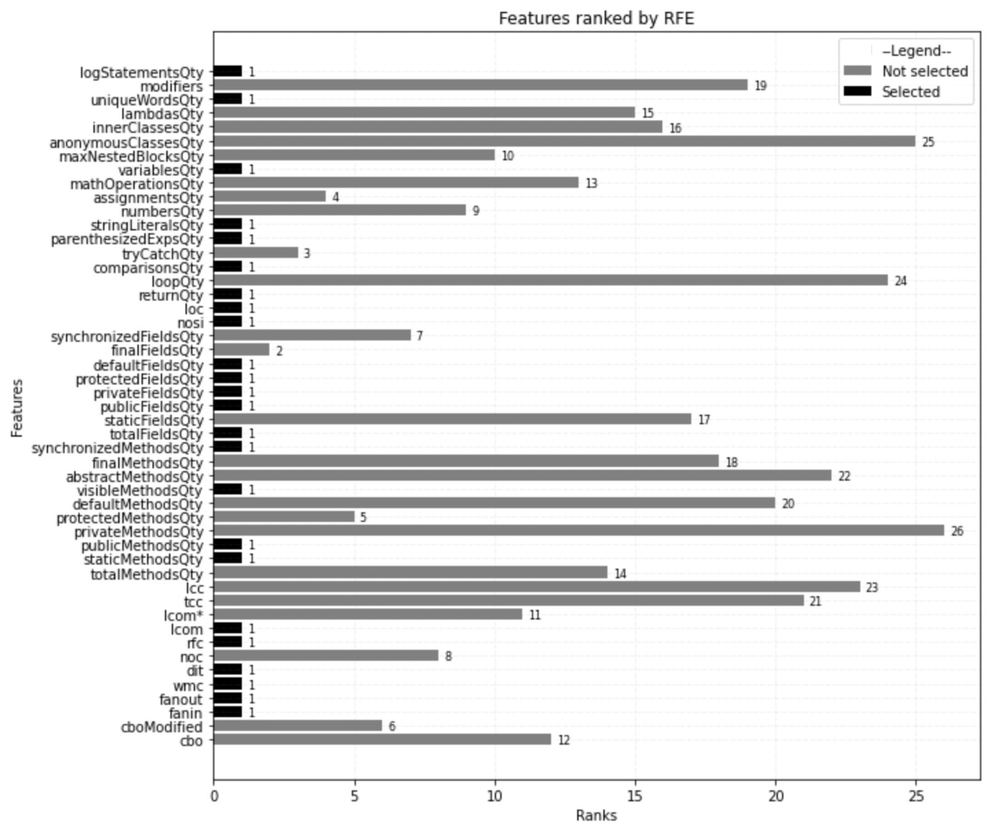
Data 07 00127 g005
Figure 6. Features ranked by Recursive Feature Elimination.
Data 07 00127 g006
Figure 7. Confusion matrix for all learners in predicting vulnerable status (Tomcat–RFE).
Data 07 00127 g007
Figure 8. Confusion matrix for all learners in predicting vulnerable status (Struts–RFE).
Data 07 00127 g008
Figure 9. Confusion matrix for all learners in predicting vulnerable status (Tomcat–SFS).
Data 07 00127 g009
Figure 10. Confusion matrix for all learners in predicting vulnerable status (Struts–SFS).
Data 07 00127 g010
Figure 11. Confusion matrix for all learners in predicting severity (Tomcat–SFS).
Data 07 00127 g011
Figure 12. Confusion matrix for all learners in predicting severity (Struts–SFS).
Data 07 00127 g012
Figure 13. Confusion matrix for all learners in predicting severity (Tomcat–RFE).
Data 07 00127 g013
Figure 14. Confusion matrix for all learners in predicting severity (Struts–RFE).
Data 07 00127 g014
Figure 15. AUC-ROC curve for all learners (Tomcat).
Data 07 00127 g015
Figure 16. AUC-ROC curve for all learners (Struts).
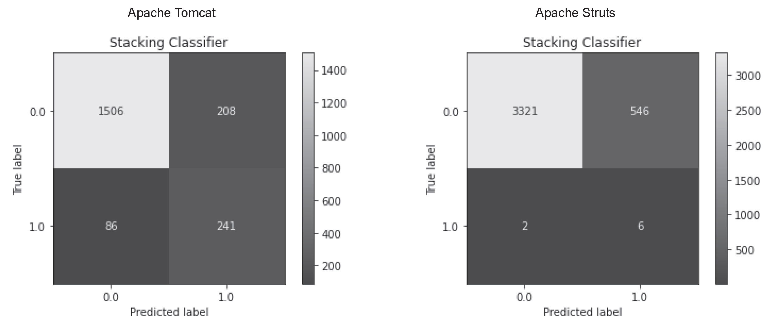
Data 07 00127 g016
Figure 17. Confusion matrix for Stacking classifier in predicting vulnerable status.
Data 07 00127 g017
Figure 18. Confusion matrix for Stacking classifier in predicting severity.
Data 07 00127 g018
Figure 19. AUC-ROC curve for Stacking classifier.
Data 07 00127 g019
Figure 20. Confusion matrix for cross-version experiments in predicting vulnerable status (Tomcat (1)–(3)).
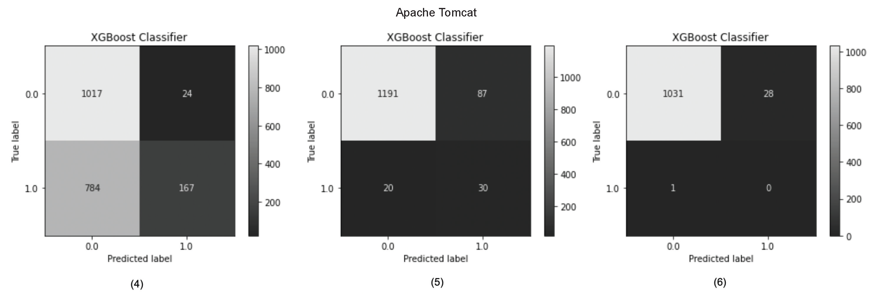
Data 07 00127 g020
Figure 21. Confusion matrix for cross-version experiments in predicting vulnerable status (Tomcat (4)–(6)).
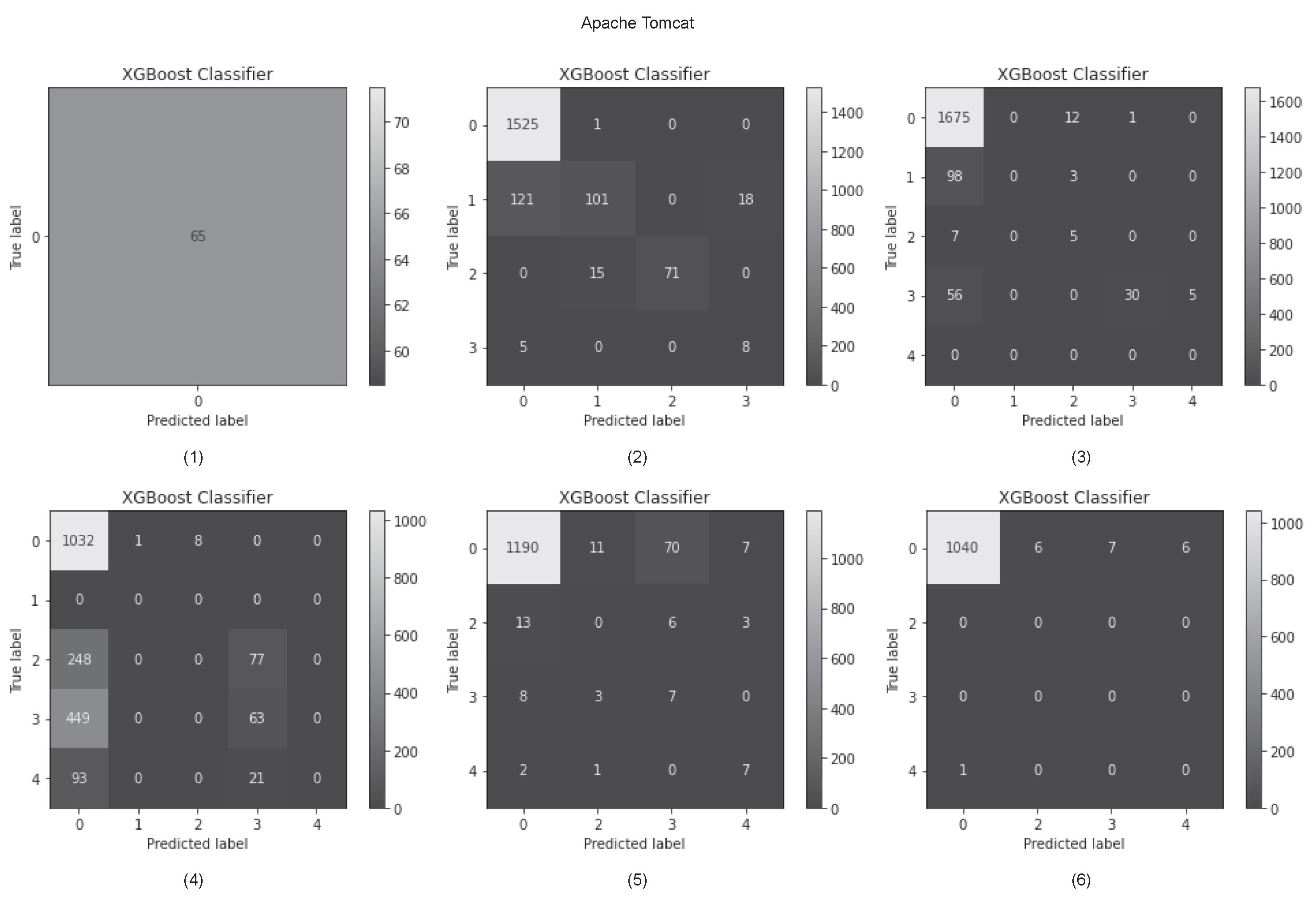
Data 07 00127 g021
Figure 22. Confusion matrix for cross-version experiments in predicting severity (Tomcat).
Data 07 00127 g022
Figure 23. Confusion matrix for cross-version experiments in predicting vulnerable status (Struts (1)–(4)).
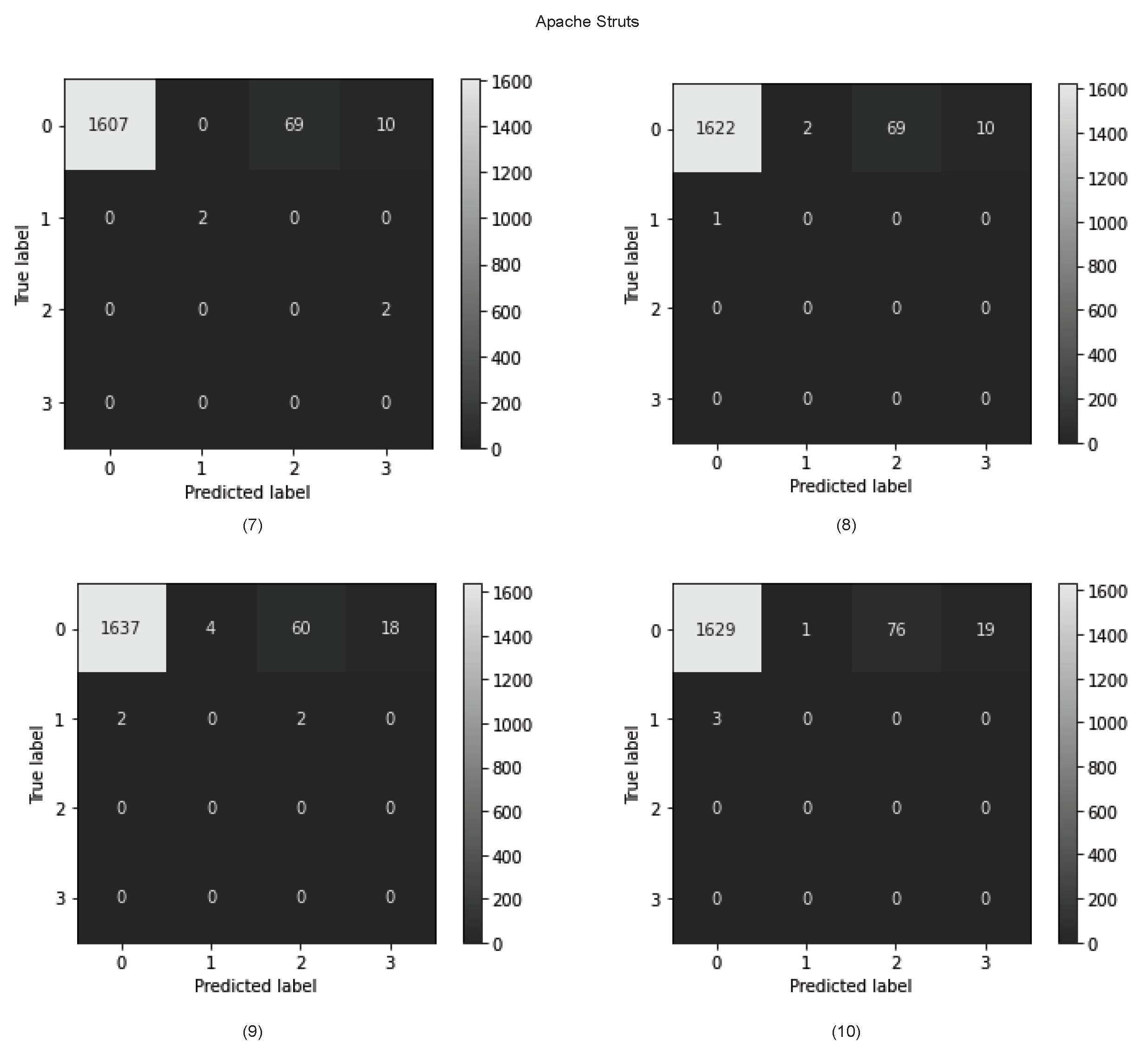
Data 07 00127 g023
Figure 24. Confusion matrix for cross-version experiments in predicting vulnerable status (Struts (5)–(8)).
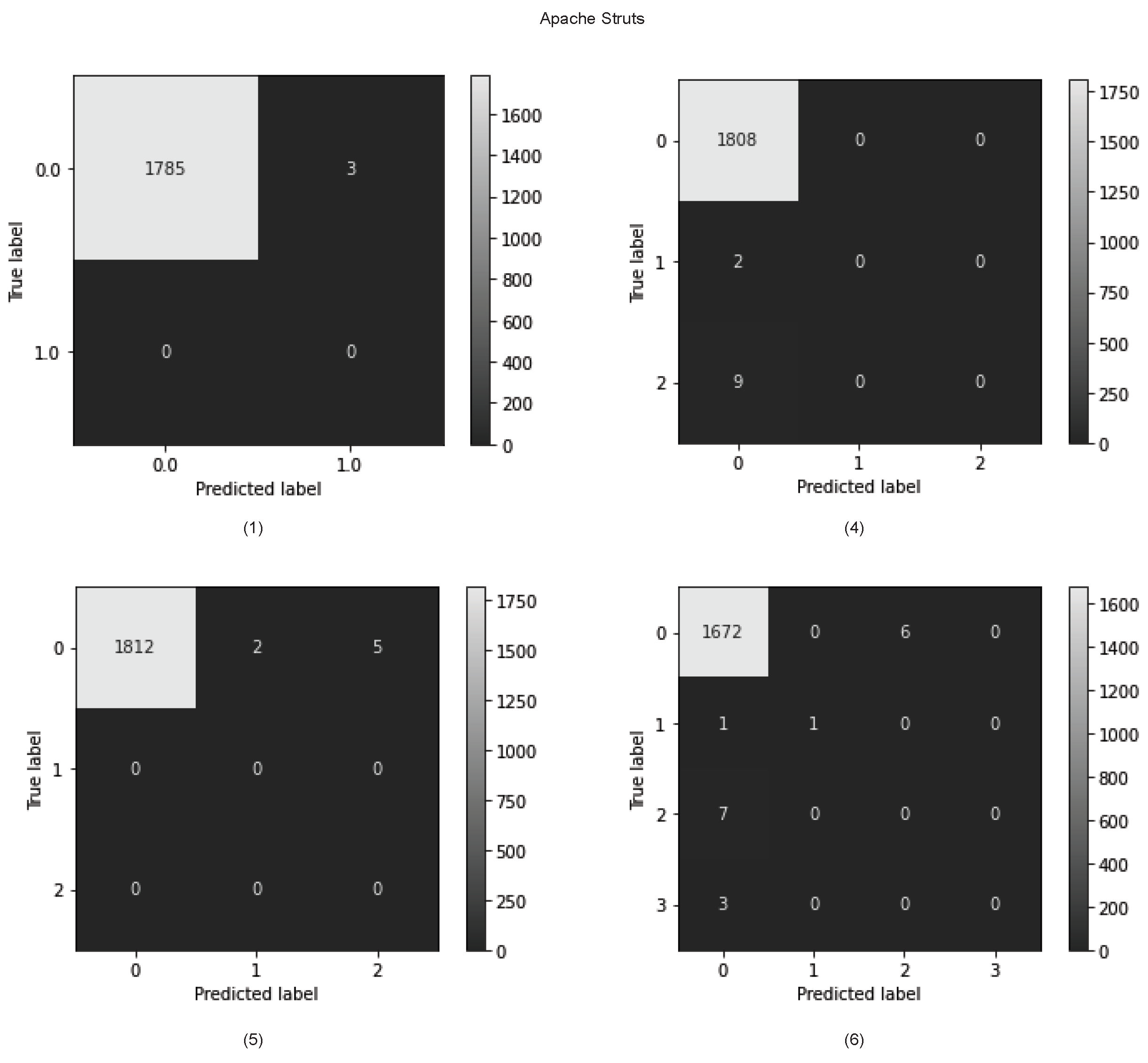
Data 07 00127 g024
Figure 25. Confusion matrix for cross-version experiments in predicting vulnerable status (Struts (9)–(10)).
Data 07 00127 g025
Figure 26. Confusion matrix for cross-version experiments in predicting severity (Struts (1), (4)–(6)).
Data 07 00127 g026
Figure 27. Confusion matrix for cross-version experiments in predicting severity (Struts (7)–(10)).
Data 07 00127 g027
Figure 28. AUC-ROC curve for Vulnerable (Tomcat).
Data 07 00127 g028
Figure 29. AUC-ROC curve for Severity (Tomcat).
Data 07 00127 g029
Figure 30. AUC-ROC curve for Title (Tomcat).
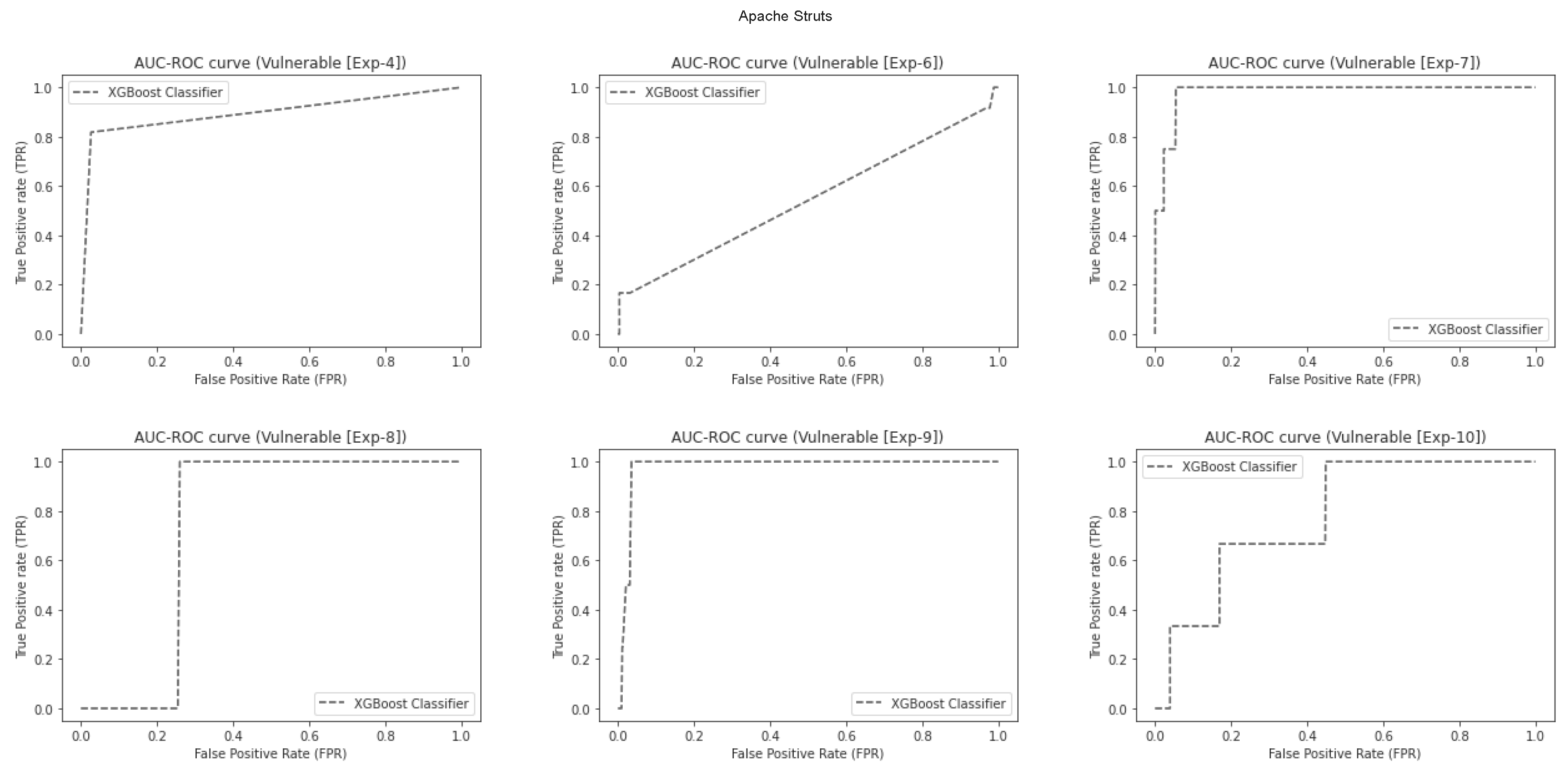
Data 07 00127 g030
Figure 31. AUC-ROC curve for Vulnerable (Struts).
Data 07 00127 g031
Figure 32. AUC-ROC curve for Severity (Struts).
Data 07 00127 g032
Figure 33. AUC-ROC curve for Title (Struts).
Data 07 00127 g033
Figure 34. Confusion matrix for cross-project experiments in predicting vulnerable status; (1) Train on Tomcat, test on Struts; (2) Train on Struts, test on Tomcat.
Data 07 00127 g034
Figure 35. Confusion matrix for cross-project experiments in predicting severity; (1) Train on Tomcat, test on Struts; (2) Train on Struts, test on Tomcat.
Data 07 00127 g035
Figure 36. AUC-ROC curve for RQ4.
Data 07 00127 g036
Table 1. List of static source code metrics [12].
MetricsDefinitions
anonymousClassesQtyNumber of anonymous classes in a class.
assignmentsQtyHow often each variable was used inside each class.
CBOCoupling Between Objects. The number of dependencies in a class.
comparisonsQtyRepresent the comparison operators in a class.
defaultFieldsQtyNumber of fields of default types.
DITDepth of Inheritance Tree. Number of fathers in a class.
fieldQtyHow often each local field was used inside each class.
finalFieldsQtyNumber of fields of final types.
HasJavadocWhether the source code has JavaDoc or not.
innerClassesQtyNumber of inner classes in a class.
lambdsQtyNumber of lambda expressions in a class.
LCCLoose Class Cohesion. Same as TCC but also includes the number of indirect connections between visible classes for the cohesion calculation.
LCOMLack of Cohesion of Methods Count of the number of method pairs whose similarity is 0.
LOCLines of Code. Total lines of code in a class.
logStatementsQtyCount of log statements in a class.
loopQtyRepresent the number of loops in a class.
mathOperationsQtyRepresent the number of arithmetic symbols in a class.
maxNestedBlocksQtyMax Nested Blocks. The highest number of blocks nested within each other.
Method InvocationsNumber of directly invoked methods, variations are local invocations and indirect local invocations.
NoSINumber of Static Invocations. The number of invocations to static methods but is limited to JDT
resolved methods.
numbersQtyRepresent the number of numeric literals in a class.
paranthesizedExpsQtyRepresent the number of parenthesized expressions in a class.
privateMethodsQtyWhether a class is private
protectedFieldsQtyNumber of fields of protected types.
protectedMethodsQtyWhether a class is protected.
returnQtyRepresent the number of return statements in a class.
RFCResponse for a Class. The number of unique method invocations in a class but fails with
overloaded methods.
stringLiteralsQtyRepresent the number of string literals in a class.
synchronizedMethodsQtyNumber of synchronized methods in a class.
TCCTight Class Cohesion. The cohesion of a class and results are delivered between 0 and 1.
totalFieldsQtyNumber of total fields.
totalMethodsQtyNumber of Methods. The number of methods of various return types and scopes.
tryCatchQtyRepresent the try and catch statements used in a class.
uniqueWordsQtyCount of unique words in a class.
variablesQtyRepresent the number of variables in a class.
visibleMethodsQtyNumber of Visible Methods. The number of non-private methods.
WMCWeight Method Class. Also known as McCabe’s complexity, it counts the number of branch instructions in a class.
Table 2. Features selected by SFS and RFE on both the datasets.
Apache Tomcat Apache Struts2-Core
SFSRFESFSRFE
LCOMCBOCBOvisibleMethodsQty
TCCWMCFanInabstractMethodsQty
LCCRFCNOCfinalMethodsQty
staticMethodsQtyLCOMLCOMsynchronizedMethodsQty
privateMethodsQtyTCCTCCtotalFieldsQty
protectedMethodsQtyLCCLCCstaticFieldsQty
defaultMethodsQtyprivateMethodsQtytotalMethodsQtypublicFieldsQty
visibleMethodsQtystaticFieldsQtystaticMethodsQtyfinalFieldsQty
abstractMethodsQtypublicFieldsQtyprivateMethodsQtysynchronizedFieldsQty
finalMethodsQtyprivateFieldsQtydefaultMethodsQtyNoSI
synchronizedMethodsQtyprotectedFieldsQtyabstractMethodsQtyLOC
staticFieldsQtydefaultFieldsQtyfinalMethodsQtyreturnQty
publicFieldsQtyfinalFieldsQtysynchronizedMethodsQtyparenthesizedExpsQty
protectedFieldsQtyNoSIprivateFieldsQtystringLiteralsQty
defaultFieldsQtyLOCprotectedFieldsQtynumbersQty
finalFieldsQtycomparisonsQtydefaultFieldsQtyassignmentsQty
synchronizedFieldsQtyparenthesizedExpsQtysynchronizedFieldsQtymathOperationsQty
loopQtystringLiteralsQtyloopQtyvariablesQty
anonymousClassesQtynumbersQtyparenthesizedExpsQtymaxNestedBlocksQty
innerClassesQtyvariablesQtyanonymousClassesQtyanonymousClassesQty
lambdasQtyuniqueWordsQtyinnerClassesQtyinnerClassesQty
modifiersmodifierslambdasQtylambdasQty
modifiersuniqueWordsQty
logStatementsQtymodifiers
Table 3. Performance metrics for predicting vulnerable status (0 or 1).
Tomcat SFS RFE
Accuracy in %Precision in %Recall in %Accuracy in %Precision in %Recall in %
DT73.737.488.174.540.685.4
LR85.755.674.183.553.572.5
NB86.157.958.183.353.761.2
XGB97.589.596.198.19297.8
Struts
DT78.10.972.781.70.557.1
LR86.61.572.787.80.642.8
NB590.581.889.60.214.2
XGB99.526.636.399.628.528.5
Table 4. Performance in predicting the severity of the vulnerability.
Tomcat SFS RFE
Accuracy in %Precision in %Recall in %Accuracy in %Precision in %Recall in %
DT71.845.355.659.945.564
LR65.438.467.269.236.960.9
NB30.633.447.736.739.150.3
XGB93.975.988.393.874.985.6
Struts
DT74.825.690.17925.369.7
LR75.825.690.384.925.454.5
NB14.225.371.385.925.538.1
XGB99.657.767.799.65341.6
Table 5. Performance in predicting the title (type) of the vulnerability.
Tomcat SFS RFE
Accuracy in %Precision in %Recall in %Accuracy in %Precision in %Recall in %
DT2.40.0142.691.19.5
LR42.223.458.256.324.164.3
NB1626.746.213.825.248
XGB9458.573.593.455.569.1
Struts
DT77.911.630.862.812.945.3
LR86.712.823.588.612.243.5
NB43.612.221.551.711.227.9
XGB99.524.924.999.524.924.9
Table 6. Stacking classifier performance in Apache Tomcat.
TomcatAccuracy in %Precision in %Recall in %
Vulnerable85.585.585.5
Severity75.375.375.3
Title53.153.153.1
Table 7. Stacking classifier performance in Apache Struts2-core.
StrutsAccuracy in %Precision in %Recall in %
Vulnerable85.885.885.8
Severity94.194.194.1
Title98.298.298.2
Table 8. Cross-version prediction in Apache Tomcat.
Vulnerable
Exp. No.Accuracy in %Precision in %Recall in %
1100100100
290.899.449.9
391.876.934.3
459.487.417.5
591.925.660
697.200
Severity
1100100100
291.477.371.5
390.342.634.7
454.919.122.2
590.636.950.5
698.124.924.5
Title
1100100100
289.951.561.5
3923432.4
451.747
588.978.9
697.797.797.7
Table 9. Cross-version prediction on Struts2-core.
Vulnerable
Exp. No.Accuracy in %Precision in %Recall in %
199.800
210000
310000
499.300
599.800
699.200
799.430.7100
899.500
999.528.550
1099.400
Severity
199.899.899.8
2100100100
3100100100
499.399.399.3
599.799.799.7
699.399.399.3
799.499.499.4
899.599.599.5
999.599.599.5
1099.499.499.4
Title
199.899.899.8
2100100100
3100100100
499.399.399.3
599.899.899.8
699.299.299.2
799.499.499.4
899.599.599.5
999.599.599.5
1099.499.499.4
Table 10. (Exp 1) Train on Tomcat, test on Struts; (Exp 2) Train on Struts, test on Tomcat.
Exp 1Accuracy in %Precision in %Recall in %
Vulnerable98.20.64.5
Severity78.412.49.8
Title000
Exp 2
Vulnerable6229.187.4
Severity32.312.14.8
Title20.93.11.5
Table 11. Performance in predicting the vulnerable status (undersampled).
Tomcat SFS RFE
Accuracy in %Precision in %Recall in %Accuracy in %Precision in %Recall in %
DT72.937.885.372.536.586
LR8453.369.982.448.778.1
NB83.652.860.383.550.963.9
XGB94.678.794.995.78197.9
Struts
DT79.70.655.571.20.890.9
LR74.10.677.775.50.981.8
NB77.50.444.482.41.172.7
XGB80.60.655.574.70.981.8
Table 12. Performance in predicting the severity (undersampled).
Tomcat SFS RFE
Accuracy in %Precision in %Recall in %Accuracy in %Precision in %Recall in %
DT71.571.571.566.366.366.3
LR64.264.264.265.265.265.2
NB28.428.428.421.221.221.2
XGB71.571.571.568.868.868.8
Struts
DT66.266.266.247.447.447.4
LR50505021.621.621.6
NB37.937.937.928.128.128.1
XGB39.439.439.4252525
Table 13. Performance in predicting the title of vulnerability (undersampled).
Tomcat SFS RFE
Accuracy in %Precision in %Recall in %Accuracy in %Precision in %Recall in %
DT4.54.54.5555
LR13.613.613.615.415.415.4
NB8885.95.95.9
XGB13.513.513.512.612.612.6
Struts
DT1.21.21.217.517.517.5
LR1.31.31.35.15.15.1
NB0.10.10.10.50.50.5
XGB0.60.60.60.10.10.1
Table 14. Stacking classifier performance in Apache Tomcat (undersampled).
TomcatAccuracy in %Precision in %Recall in %
Vulnerable7741.587.2
Severity66.566.566.5
Title10.610.610.6
Table 15. Stacking classifier performance in Apache Struts (undersampled).
StrutsAccuracy in %Precision in %Recall in %
Vulnerable70.410086.6
Severity69.269.269.2
Title6.46.46.4
Table 16. Cross-version prediction performance in Apache Tomcat (undersampled).
Vulnerable
Exp. No.Accuracy in %Precision in %Recall in %
197.100
291.700
396.400
492.37100
595.100
695.900
Severity
198.498.498.4
267.667.667.6
371.771.771.7
434.734.734.7
5727272
6808080
Title
176.976.976.9
266.366.366.3
3424242
423.923.923.9
531.431.431.4
630.930.930.9
Table 17. Cross-version prediction performance in Apache Struts (undersampled).
Vulnerable
Exp. No.Accuracy in %Precision in %Recall in %
192.600
295.300
391.900
495.411.8100
594.500
696.6416.6
7811.2100
869.30.1100
979.71.1100
1079.70.233.3
Severity
196.596.596.5
295.195.195.1
391.591.591.5
494.894.894.8
570.970.970.9
692.492.492.4
76.56.56.5
854.654.654.6
970.270.270.2
1056.756.756.7
Title
1888888
2959595
3929292
492.392.392.3
5939393
687.687.687.6
799.799.799.7
899.999.999.9
931.631.631.6
1023.823.823.8
Table 18. Cross-project prediction performance (undersampled). (Exp 1) Train on Tomcat, test on Struts; (Exp 2) Train on Struts, test on Tomcat.
Exp 1Accuracy in %Precision in %Recall in %
Vulnerable97.50.120.4
Severity88.488.488.4
Title0.10.10.1
Exp 2
Vulnerable67.331.983.2
Severity29.129.129.1
Title18.618.618.6
Table 19. Performance of all learners in predicting vulnerable status in both datasets. (Weighted-average).
Tomcat SFS RFE
Accuracy in %Precision in %Recall in %Accuracy in %Precision in %Recall in %
DT7795.6777795.877
LR83.895.783.884.295.884.2
NB89.895.289.890.395.290.3
XGB96.79796.795.796.495.7
Struts
DT81.999.781.983.699.783.6
LR86.999.686.984.799.784.7
NB1499.51473.899.873.8
XGB99.699.799.699.699.799.6
Table 20. Performance of all learners in predicting severity in both datasets. (Weighted-average).
Tomcat SFS RFE
Accuracy in %Precision in %Recall in %Accuracy in %Precision in %Recall in %
DT58.795.958.480.195.880.1
LR85.695.885.682.199.682.1
NB25.395.434.439.39639.3
XGB68.596.166.370.596.470.5
Struts
DT84.599.884.583.999.583.9
LR83.799.783.780.299.480.2
NB19.199.619.180.799.680.7
XGB8899.7889499.594
Table 21. Performance of all learners in predicting title of the vulnerability in both datasets. (Weighted-average).
Tomcat SFS RFE
Accuracy in %Precision in %Recall in %Accuracy in %Precision in %Recall in %
DT8.618.612.400
LR35.50047.196.147.1
NB9.392.99.335.596.135.5
XGB61.596.161.566.796.166.7
Struts
DT70.399.770.361.799.761.7
LR46.699.646.661.299.661.2
NB31.899.631.843.699.743.6
XGB95.399.795.391.999.791.9
Table 22. Stacking classifier performance in Apache Tomcat. (Weighted-average).
TomcatAccuracy in %Precision in %Recall in %
Vulnerable81.59683.5
Severity8395.883
Title89.995.389.9
Table 23. Stacking classifier performance in Apache Struts. (Weighted-average).
StrutsAccuracy in %Precision in %Recall in %
Vulnerable96.599.896.5
Severity99.499.899.4
Title99.699.799.6
Table 24. Cross-version prediction performance in Apache Tomcat. (Weighted-average).
Vulnerable
Exp. No.Accuracy in %Precision in %Recall in %
1100100100
292.392.192.3
387.383.587.3
464.668.264.6
580.395.980.3
680.499.780.4
Severity
1100100100
283.279.983.2
379.485.579.4
45144.251
575.195.975.1
676.999.776.9
Title
1100100100
276.775.576.7
380.982.680.9
444.737.444.7
570.195.670.1
663.799.763.7
Table 25. Cross-version prediction performance in Apache Struts. (Weighted-average).
Vulnerable
Exp. NoAccuracy in %Precision in %Recall in %
199.710099.7
299.710099.7
3100100100
499.398.799.3
599.310099.3
698.898.898.8
796.999.796.9
895.299.895.2
993.199.593.1
1092.599.792.5
Severity
199.710099.7
299.710099.7
3100100100
499.398.799.3
599.610099.6
698.998.798.9
795.299.895.2
895.199.895.1
99599.695
1094.299.694.2
Title
199.710099.7
299.710099.7
3100100100
499.398.799.3
599.610099.6
698.998.698.9
795.699.895.6
894.699.894.6
99499.794
1093.899.793.8
Table 26. Cross-project prediction performance in Apache Struts. (Weighted-average). (Exp 1) Train on Tomcat, test on Struts; (Exp 2) Train on Struts, test on Tomcat.
Exp 1Accuracy in %Precision in %Recall in %
Vulnerable95.399.695.3
Severity90.999.690.9
Title83.799.683.7
Exp 2
Vulnerable70.371.770.3
Severity69.27069.2
Title74.368.774.3
Publisher’s Note: MDPI stays neutral with regard to jurisdictional claims in published maps and institutional affiliations.

