Abstract
Multiple blood images of stressed and sheared cells, taken by a Lorrca Ektacytometery microscope, needed a classification for biomedical researchers to assess several treatment options for blood-related diseases. The study proposes the design of a model capable of classifying these images, with high accuracy, into healthy Red Blood Cells (RBCs) or Sickle Cells (SCs) images. The performances of five Deep Learning (DL) models with two different optimizers, namely Adam and Stochastic Gradient Descent (SGD), were compared. The first three models consisted of 1, 2 and 3 blocks of CNN, respectively, and the last two models used a transfer learning approach to extract features. The dataset was first augmented, scaled, and then trained to develop models. The performance of the models was evaluated by testing on new images and was illustrated by confusion matrices, performance metrics (accuracy, recall, precision and f1 score), a receiver operating characteristic (ROC) curve and the area under the curve (AUC) value. The first, second and third models with the Adam optimizer could not achieve training, validation or testing accuracy above 50%. However, the second and third models with SGD optimizers showed good loss and accuracy scores during training and validation, but the testing accuracy did not exceed 51%. The fourth and fifth models used VGG16 and Resnet50 pre-trained models for feature extraction, respectively. VGG16 performed better than Resnet50, scoring 98% accuracy and an AUC of 0.98 with both optimizers. The study suggests that transfer learning with the VGG16 model helped to extract features from images for the classification of healthy RBCs and SCs, thus making a significant difference in performance comparing the first, second, third and fifth models.
Keywords:
deep learning; sickle cells; transfer learning; VGG16; Resnet50; confusion matrix; Adam optimizer; ROC curve; SGD 1. Introduction
Over the last decade, the rapid pace of development in Artificial Intelligence (AI) has raised its prominence by creating opportunities to improve performance in various industries and businesses [1]. In contrast to conventional programming, the success of AI lies in the effective implementation of the algorithms having the ability to learn by trial and error and increase their performance with time [2]. AI is an umbrella term that refers to imitating human intelligence in machines [3]. Machine Learning (ML) and Deep Learning (DL) are two other concepts used in conjunction with AI. If an intelligent program enables a machine to behave human-like, it can be regarded as AI but not ML if it does not learn from data automatically [4].
DL is a specialized instance of ML that works on the principle of biological neural networks [5]. It has shown remarkable gains in many domains [4] with significant dominance over conventional ML algorithms [5] due to a higher level of abstraction. The multiple layers in DL models are composed of linear and non-linear transformations. The increased popularity of DL models is due to expansion in software and hardware infrastructure [6].
The exponential rise in data volume has revealed the limitations of ML algorithms in analyzing the volume of data [7]. The use of DL techniques becomes effective when the training dataset is voluminous. Due to the leading-edge performance in different domains such as e-commerce [8], speech recognition [9,10], health monitoring [8] and computer vision [11,12], DL has gained worldwide appreciation from the academic community [13].
Generally, ML and DL algorithms are used to accomplish two classical statistical tasks of classification and regression on the provided dataset. Data may be structured (e.g., table with numeric values) or unstructured (e.g., images or HTML). According to a study [14], the exponential rise in digital activities signifies unstructured data, which is expected to constitute 95% of digital data by 2020. Unstructured data does not follow any format or formal data model, which makes it challenging to process and interpret for value extraction. In the medical industry, unstructured healthcare data has tremendous potential to extract valuable insight for improving healthcare service and quality [15].
Medical imaging is a research area facing rapid growth due to its significance in the early diagnosis of disease [3]. Multiple regression and Neural Networks models can be used to predict the possibility of a patient having a specific disease in the future [16]. There are numerous studies conducted for the classification and prediction of multiple diseases using ML and DL algorithms, such as the image classification of MRI brain images [17], cardiovascular disease prediction [18], X-ray image classification [19] and breast cancer prediction [20]. These predictions and classifications can be helpful in early detection and diagnosis to devise early interventions for effectively managing diseases. Sickle Cell disease is a hereditary hemolytic disorder caused by an abnormal hemoglobin structure, which polymerizes upon deoxygenation [21]. Such a condition distorts the patient’s RBCs into a sickle or crescent shape [22]. These sickle RBCs clutter together, causing resistance in flow through vessels and causing stroke, which is one of the most devastating complications [23].
This study aims to develop a classification model for microscopic images of Sickle Cells (SCs) and healthy Red Blood Cells (RBCs) using a Convolutional Neural Network (CNN), which is a DL algorithm. CNNs are widely used for image processing as a powerful tool because of their performance in image classification with higher accuracy [24]. Using a CNN for image processing does not require manual feature extraction (from the image) or segmentation. It has millions of parameters to be learned for estimation, making it computationally expensive and thus raising the need for Graphical Processing Units (GPU) to train the model. The computing capability of GPU is higher than the traditional CPU cores [25]. If conducted from scratch, model training is time-consuming and needs a large and labeled dataset for training, preparing the model for classification [26].
For the classification of SCs and RBCs, five models or approaches were used. The first, second and third models comprised one, two and three blocks of the CNN, respectively, and the fourth and fifth models used a transfer learning approach. This study also shows how the transfer learning approach can be used for better cell classification with improved accuracy. In transfer learning, two popular pre-trained models, VGG16 and Resnet50, were used for feature extraction, and a classifier layer was added for image classification as either an SC or healthy RBC image. The concept of using a pre-trained model was used to borrow the model weights from the pre-trained models developed for Computer Vision (CV) standard datasets.
2. Related Research
Several techniques have been employed to diagnose or classify SCs, such as Image processing, Machine Learning and Deep Learning methods. In 2014, Patil and Khot [27] introduced an image-processing-based technique for detecting, counting and segregating abnormal blood cells using form factor calculation. Some significant image processing algorithms used in their proposed technique are the Sobel edge mask, morphological techniques such as erosion and dilation, and watershed transformation. The proposed approach managed to achieve an accuracy of 83% in counting blood cells. Maity et al. [28] proposed an ensemble-rule-based decision-making algorithm for the morphological classification of erythrocytes. The erythrocytes were first segmented from the background image using watershed transformation followed by feature extraction to detect the shape abnormality. Their model detected eight different types of abnormal erythrocytes with 97.81% accuracy and a weighted precision of 98%. Akrimi et al. [29] used the Support Vector Machine (SVM) to classify RBCs as either normal or abnormal. They applied image processing techniques to pre-process the images using optimization segmentation and mean filtering to extract RBCs’ color, texture and geometric features. The developed classifier achieved an accuracy of 99.8% with 100% sensitivity. In another study [30] of erythrocyte classification in microscopic images, SVM, KNN and Naïve Bayes classifiers achieved an accuracy of 0.946, 0.931 and 0.932, respectively. Veluchamy et al. [31] used Artificial Neural Networks (ANN) to classify sickle cells as normal or abnormal by first applying thresholding techniques and morphological operations for image segmentation. Other studies such as [32,33] also used ANN for the classification of RBCs. Tomari et al. [34] proposed a framework for the automatic classification of RBCs into overlapping, normal and abnormal clusters. Their approach comprised three blocks, namely a segmentation and processing block, a feature extraction block and a classification block. The Otsu segmentation method, with a series of post-processing filters, was used to crop RBC shapes from the background. The model achieved an average accuracy, precision and recall of 83%, 82% and 76%, respectively. Poomcokrak and Neatpisarnvani [35] proposed neural networks for SC identification. An edge detection algorithm was used to extract RBCs, followed by analyzing and classifying the individual cells using a neural network. Fadhel et al. [36] employed watershed transform and Circular Hough Transform (CHT) to identify circular-shaped normal RBCs. During the watershed segmentation, the effectiveness factor was calculated to differentiate normal and sickle cells. Chy et al. [37] used Extreme Learning Machine (ELM), SVM and KNN classifiers to classify normal and sickle cells. The approach started with image preprocessing for greyscale conversion, noise removal and image enhancement. Then, morphological operations were applied to extract geometrical and statistical features. ELM performed the best with an accuracy, precision and sensitivity of 87.73%, 95.45% and 87.5%, respectively. Alzubaidi et al. [38] proposed a CNN framework to classify RBCs into three classes, i.e., normal, abnormal and miscellaneous. Their proposed model comprised 18 layers, including 4 convolutional layers for feature extraction. After the fully connected layer, an Error-Correcting Output Code (ECOC) classifier was added for the classification task. The model achieved an accuracy of 92.06%. Similarly, studies such as [29,39] used CNNs to classify RBCs from microscopic images and gained 87.5% and 92.06% accuracy, respectively. Likewise, in a study about White Blood Cell (WBC) classification into five classes [40], a two-module weighted optimized deformable CNN (TWO-DCNN) was proposed, and the performance was compared with classical ML algorithms such as VGG16, VGG19, Inception-V3, Resnet50, support vector machine (SVM), multilayer perceptron (MLP), decision tree (DT) and random forest (RF). TWO-DCNN performed the best, with precision values of 95.7%, 94.5% and 91.6% on different datasets.
This study seeks to develop a DL classifier capable of achieving higher accuracy besides showing the use of multiple evaluation parameters such as a confusion matrix, precision, recall, f1 score and ROC curves to obtain insight into the model performance for each class. Consequently, these evaluation metrics can be used to improve the model performance by adopting measures for the class(s) with weak recall and precision values. The correctness of the diagnosis is highly dependent on the precise classification [30]. Feature extraction, therefore, plays a key role in the classifier’s performance. For better feature extraction, this research made use of the transfer learning approach, which is characterized by using the weights of pre-trained models.
The current study differs from the studies mentioned above in the following ways:
- Five CNN-based models were used, three were custom-built and the other two models used a convolutional base of two pre-trained models, namely VGG16 and Resnet50, for feature extraction.
- An undisclosed dataset was used, which was not previously worked on (see Section 3).
- Two optimizers, namely Adam and SGD, were used to compile all five models.
- The highest accuracy of 98% was achieved with the model using VGG16 for feature extraction.
3. Materials and Methods
3.1. Dataset
The images used in the study were received from RR Mechatronic BV, a Netherlands-based company specializing in hematology lab instruments and research. The blood images used in the dataset were taken by a Lorrca Ektacytometry microscope. An Ektacytometer is an instrument that applies a shear force on a suspension of RBCs while analyzing the diffraction pattern of a laser beam passing along these cells. Exerting a shear onto the cells can measure the average deformability of the cells. In this study, the used RBC images were from a sickle cell patient. The oxygen level in the sample was reduced; therefore, some cells started to show typical sickling behavior. The patient cells became rigid as the hemoglobin, due to the genetic defect in these cells, started to polymerize at low oxygen levels. This rigidifying of the RBC lies at the core of this disease. A microscope was added to observe the sickling phenomenon while the cells were under shear. To a degree, being submitted to a shear force mimics the process in the small capillaries of a sickle cell patient when the oxygen is delivered to the muscles or organs [41]. Images taken by the camera needed a classification for further study and research. The study underwent the classification of images into Healthy RBCs or SCs.
The number of received images was 450, and the dataset was expanded using image augmentation. Figure 1 shows the flow of the activities performed to train models or classifiers. The augmented dataset was analyzed to remove any damaged or faded images, leaving a total of 1085. A total of 885 images were used for training and validation, and 200 images were kept separate for the model test. Before feeding to the model, each image of the dataset was scaled down to 255. Rescaling improves the model’s ability to learn [42], during which each pixel value is transformed from (0,255) to (0,1). For model training, every image of the dataset was shaped as (300, 200, 3).
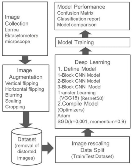
Figure 1.
Workflow.
3.2. Working with the Dataset
3.2.1. Image Augmentation
The Data Augmentation technique was used for the artificial expansion of the dataset by creating transformed versions of images by using techniques such as sharing, rotating and scaling the images [43]. This process results in an extensive dataset that is robust and less susceptible to adversarial attacks [44], as shown in Figure 2. There are different ways to implement data augmentation in Python, e.g., the imgaug library of Python was used in this study for the augmentation of the dataset. Not every technique for augmentation is valid for all types of problems, e.g., some techniques such as shearing and skewing may distort the critical features in medical imagery. Therefore, the techniques to extend the dataset must be carefully handled. Figure 2 shows the different versions of the same image after applying some augmentation techniques.
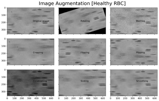
Figure 2.
Augmentations of a Healthy RBC image.
3.2.2. CNN
Artificial Intelligence has played a vital role in bridging the gap between human brains and machines in various fields. One of them is computer vision, whose main plan is to make machines visualize their environment like a human brain. It enables machines to perform tasks such as image recognition, image classification, video recognition, Natural Language Processing (NLP), recommendation systems, etc. Convolutional Neural Networks are a vital algorithm that helps perform such tasks. A CNN is a DL algorithm that takes images as input and can differentiate or classify them by assigning them weights and biases. The importance of a CNN lies in the fact that weights/features of the NN for classification tasks are implicitly learned and are not required to be passed by humans as heuristics [45]. One block of a CNN has the following four layers.
- Convolutional Layer: A convolutional layer is the first building layer of a CNN, in which a convolutional operation is performed. A convolution is the application of a filter to an input that results in activation, and repeated activations result in the construction of a feature map [46], which indicates the location and strength of a detected feature in the input. It involves the multiplication, i.e., dot product, of input with the set of weights, typically an array of input data and a two-dimensional array of weights, called a kernel or a filter. The output of this multiplication is a single value, and as the kernel is applied multiple times to the input array, it forms a two-dimensional output, which is a filtered form of the input image. This output is called a feature map [47]. The primary objective of this layer is to extract features such as edges, color and gradient orientation. The first convolutional layer typically gives low-level features, but by adding more layers, high-level features can be extracted.
- ReLU Layer: It is a convention to apply a Rectified Linear Unit Layer (ReLU) immediately after the convolutional layer to filter the information propagating through the network. The ReLU layer works as shown in Equation (1) by only giving an output of 1 when x is greater than or equal to 0 [47]:The ReLU Layer changes all negative activations to 0 to increase the system’s overall nonlinearity without affecting the receptive fields of the convolution layer.
- Pooling Layer: Pooling is a down-sampling operation mainly applied after the convolutional layer to create spatial invariance [48]. The two most common types of pooling are average and max pooling, in which average and maximum values are chosen, respectively. Max pooling is used to preserve the detected features, and average pooling down-samples the feature map. The difference between max pooling and average pooling is that the latter summarizes all features in the pooling tier, whereas the former only retains the strongest activations [49]. In this study, max pooling was used to preserve the essential features.
- Fully Connected Layer: The purpose of the fully connected layer is to transform the results of previous layers into a meaningful outcome, i.e., a label. The output of the convolutional/pooling layer is flattened to a column vector, where each entity represents which feature belongs to which label, e.g., in a classification problem of the car and mouse, features such as eyes, whiskers and tails belong to the mouse label, whereas lights, steering wheels and tires fall under the car label. The number of output nodes in the final fully connected layer is equal to the number of classes [47], e.g., in a binary classification problem, the output node is set as 1, which could be either 0 for one class or 1 for the other class.
3.2.3. Transfer Learning
In medical imagery, the use of Transfer Learning has gained popularity due to better performance over a small dataset. Transfer learning works on the idea of choosing any pre-trained model and using it after fine-tuning or as a feature extractor without any tuning. However, the last dense layer of the pre-trained model is removed and replaced with the custom classifier. Then, the weights of all other layers are set as frozen, and the network is trained typically. This technique not only prevents the hassle of creating layers from scratch but also assists with using the weights and biases of a pre-trained model and simultaneously customizing the whole network according to the dataset in use. In Python, the Keras library provides easy access to several top-performing models trained on the ImageNet dataset for image recognition and classification tasks, namely VGG16, Resnet and Inception.
The VGG architecture was developed by Simonyan and Zisserman in 2014 [50], and Resnet was proposed by Him et al. in 2015 [51]. There are more than 14 million photos and 22,000 categories in the ImageNet dataset, which were used to train these models. VGG16 and Resnet50 can be downloaded and used directly, or they can be integrated into any model based on any specific Computer Vision problem. VGG16 and Resnet50 were used for this study as pre-trained models for feature extraction with an attached binary classifier (for SC and Healthy RBC classification), as shown in Figure 3. There is a common misconception that effective Deep Learning models cannot be created without voluminous data. No one can neglect the importance of data, but transfer learning helps to reduce data demands [50].
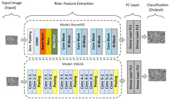
Figure 3.
Architecture view of the used pre-trained models.
3.2.4. Hyperparameters
Hyperparameters are parameters that must be carefully tuned before a specific model is trained. In Python, certain hyperparameters are already given some default values by the packages, so if the user does not provide any value, the default value is used for training [52]. The following hyperparameters were used.
- Kernel/filter size: The kernel or filter size is the matrix of weights with which the input image is convolved. Smaller kernels such as 1 × 1, 2 × 2, 3 × 3, 4 × 4 or larger ones with 5 × 5 and higher dimensions can be used. Small-sized kernels are preferred due to reduced computational costs and weight sharing, causing lesser weights for backpropagation. Similarly, a small-sized filter is used when objects in an image are differentiated by small and local features. In this study, a small-sized 3 × 3 kernel was used, which is considered an optimal choice by practitioners.
- Padding: Padding is the process of adding rows and columns of zeroes, performed after convolution, to keep the spatial size of the input image constant. In Python, the padding is one of the parameters of Conv2D, which can be ‘same’ or valid. Setting padding = ‘same’ keeps the output size the same as the input size by padding zeroes evenly on all sides. However, if the value of the padding is chosen as valid, it shrinks the output image towhere n is the dimension of the input image, f is the filter size, s is the stride and ceil rounds off the value to the nearest integer. The ‘same’ padding was chosen for the study, as it could help improve model performance by preventing data loss [53].
- Optimizer: The optimizer can be conceptualized as a mathematical function used as an argument to the compile function during model training in Python. The performance of the model is usually measured by comparing the predicted output value with the actual output value. Cross-entropy loss is one such indicator used to gauge model performance. It is a continuous function with an initial positive value that becomes zero when the predicted value is the same as the desired value [54]. The optimizer facilitates optimization by bringing the cross-entropy loss value as close to zero as possible. Optimizers use a gradient descent algorithm to iteratively minimize the objective function J(θ) by following the gradient and by updating the parameters in the opposite direction of the gradient of the objective function ∇θJ(θ) concerning the parameters [54,55].
At each iteration, the error, after comparing the predicted and the desired output, is backpropagated. In this study, each model was compiled twice with the following two optimizers to observe the model performance.
- Stochastic Gradient Descent (SGD) is the simplest form of gradient descent, in which parameter θ is updated at each step t according to the rule provided in Equation (3).where is the gradient of the objective function, and η is the learning rate.
- The second used optimizer was Adaptive Moment Estimation (Adam), which works by computing adaptive learning rates for each parameter. It saves exponentially decaying average values of the past gradient () and past squared gradient (), computed as shown in Equations (4) and (5).
and are decay rates with values near zero, causing and to be biased towards zero. To overcome this, biased corrected terms for and are computed and used to update weight by Adam, as shown in Equation (6)
3.3. Model Performance
3.3.1. Confusion Matrix
The confusion matrix provides a holistic view of the performance of a classification model. The matrix compares the true values with those predicted by the model. Figure 4 shows the heatmap visualization of the confusion matrix using the sklearn library of Python. It comprises two rows and two columns representing two classes (Healthy RBCs and SCs) with correct and incorrect predictions. The following four characteristics were used to define the measurement matrix of the classifier.
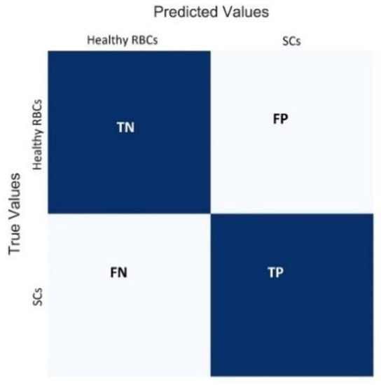
Figure 4.
Confusion matrix.
- True Negatives (TN): the count of the outcomes which are originally Healthy RBCs and are truly predicted as Healthy RBCs.
- False Positives (FP): the number of images that are originally Healthy RBCs but are predicted falsely as SCs. This error is named as a type 1 error.
- False Negatives (FN): the count of SC images, which are falsely predicted as Healthy RBCs, also known as a type 2 error.
- True Positives (TP): the count of SC images which are truly predicted as SCs.
3.3.2. Classification Report
After the confusion matrix is drawn, the performance metrics (accuracy, recall, precision and f1 score) of the models can be retrieved using classification report. The classification report can be imported from the sklearn library into Python using sklearn.metrics import classification_report. The values of the performance metrics are calculated on the basis of TN, FP, FN and TP.
- Accuracy is the measure of all correctly classified images and is represented as the ratio of correctly classified images to the total number of images in the test dataset, as shown in Equation (7).
- Precision is the correctly predicted positive images out of all positive images. For instance, it can be defined as the ratio of correctly classified images as SCs to the total number of images predicted as SCs, as shown in Equation (8).
- Recall is calculated by dividing the correctly classified images (of a class) by the total number of images belonging to that class.
- f1 score is the weighted sum of precision and recall with a minimum value of 0 and a maximum value of 1. It provides a better measure of incorrectly classified images than the accuracy metric. The value of the f1 score is measured by Equation (10).
3.3.3. Receiver Operating Characteristics (ROC) Curves
ROC curves demonstrate the performance of a model to distinguish two classes by plotting the True Positive Rate (TPR) on the y-axis against the False Positive Rate (FPR) on the x-axis. The area under the ROC curve is also known as AUC, which is the accuracy measure of the model to classify between two groups. A TPR of 1 and FPR of 0 show perfect classification for all test images, whereas a TPR of 0 and FPR of 1 indicate the worst operating point with incorrect classifications. Equations (11) and (12) show the calculation of FPR and TPR, respectively.
4. Results
A summary of the models’ training is shared in Table 1, which gives an overview of the training/validation loss and accuracy of models using Adam and SGD optimizers. The first model with both optimizers showed the same training and validation accuracy values, but the validation loss of the model with Adam (6.9) was less than SGD (8.0). For the two-block CNN model, the Adam optimizer did not appear to improve its numbers significantly. The validation loss remained at 6.9, but there was a slight fall in the training loss value from 8.2 to 7.9. Likewise, the training and validation accuracy with the Adam optimizer did not exceed 0.50 in the second model. In the two-block CNN model, SGD showed better figures. The training and validation loss values significantly fell to low scores of 0.03 and 0.17 but with a good rise in training and validation accuracy of 0.98 and 0.89, respectively. In the three-block CNN model with Adam, the training and validation loss increased to 8.1 and 7.5, respectively. The learning of the three-block CNN model with SGD showed better scores than the Adam optimizer, with a validation loss value of 0.3 and validation accuracy of 0.6.

Table 1.
Model learning comparison of transfer learning with basic models.
Transfer learning was used for the fourth and fifth models, and two pre-trained models, VGG16 and Resnet50, were used. The VGG16 models with both optimizers showed the best results by reducing the training and validation losses to 0 while amplifying the training and validation accuracy to 1. Despite having a good validation accuracy of 1 and 0.9255 with the Adam and SGD optimizers, Resnet50 performed poorer than VGG16 because of the higher validation loss of 0.2488 and 0.6785.
After training and fitting the model, diagnostic plots or learning curves were used to represent the model’s learning. Figure 5 shows the accuracy and loss curves during the training and validation of the first two models using the Matplotlib library of Python.
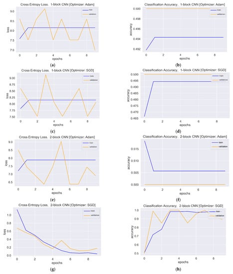
Figure 5.
Loss and accuracy plots: (a) Loss plot of one-block CNN using Adam. (b) Accuracy plot of one-block CNN using Adam. (c) Loss plot of one-block CNN using SGD. (d) Accuracy plot of one-block CNN using SGD. (e) Loss plot of two-block CNN using Adam. (f) Accuracy plot of two-block CNN using Adam. (g) Loss plot of two-block CNN using SGD. (h) Accuracy plot of two-block CNN using SGD.
The accuracy and loss curves of the three-block model trained with Adam and SGD optimizers are presented in Figure 6.
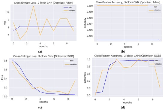
Figure 6.
Loss and accuracy plots: (a) Loss plot of three-block CNN using Adam. (b) Accuracy plot of three-block CNN using Adam. (c) Loss plot of three-block CNN using SGD. (d) Accuracy plot of three-block CNN using SGD.
Two pre-trained models, VGG16 and Resnet50, were used for feature extraction in the fourth and fifth models, respectively. The learning curves of these models with both optimizers are shown in Figure 7.
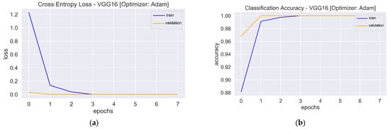
Figure 7.
Loss and accuracy plots: (a) Loss plot of VGG16 using Adam. (b). Accuracy plot of VGG16 using Adam. (c) Loss plot of VGG16 using SGD. (d) Accuracy plot of VGG16 using SGD. (e) Loss plot of Resnet50 using Adam. (f) Accuracy plot of Resnet50 using Adam. (g) Loss plot of Resnet50 using SGD. (h) Accuracy plot of Resnet50 using SGD.
5. Discussion
The one-block CNN model (Figure 5) with Adam and SGD optimizers showed no improvement during 10 epochs. Both optimizers’ training and validation accuracy plots showed a straight horizontal line at 0.49 and 0.50, respectively. Similarly, the training loss values with both optimizers were very high (>8) and stayed the same until the 10th epoch, indicating that the model had not enough capacity to capture the variability of the data, or it was unable to learn the training dataset, which is called underfitting [56]. The plots of validation loss for both optimizers seemed stationary, with a few big spikes. The cross-entropy loss of the model should have had a downward trend to show a decrease in loss as training proceeded. As the value of the loss became lower, the model became better. The accuracy and loss plots for the second model with Adam were almost similar to the first model. However, SGD showed improvement, with the validation loss value starting from a value of 0.67 and gradually falling to 0.17 in the last epoch. Similarly, the accuracy curve showed an upward trend, with a starting value of 0.50 and an end value of 0.89. The loss and accuracy plots showed a good fit with fluctuations or noisy movements that indicated unrepresentative validation images. The training dataset could not provide adequate information to assess the model’s generalization ability. The three-block CNN model with the Adam optimizer showed the same underfit loss plot. The SGD optimizer with the three-block CNN showed similar performance to the two-block CNN, but the validation loss increased, and the accuracy fell. The learning curve of validation loss showed a sudden deviation from training loss, and likewise, the validation accuracy curve was set apart from training accuracy after the eighth epoch. In that case, training could be halted when the curve showed over-fitting dynamics. The loss and accuracy curves with transfer learning showed a good fit as training and validation lines overlapped each other and reached a point of stability after the third and first epoch with the Adam and SGD optimizers, respectively. The trained models were evaluated on 200 images, and the performance metrics are shown in Table 2.
Table 2.
Comparison of the model’s performance metrics.
For the one-block CNN model, the SGD optimizer performed better than the Adam optimizer with a 51% test accuracy. With Adam, the model classified all test images as Healthy RBCs with 0.50 precision, an inability to recall SCs and hence an f1 score of 0 for SCs. The f1 score for Healthy RBCs was 0.67. However, SGD enabled the model to recall features from both classes, which may indicate the better generalization ability of SGD over Adam [57].
The accuracy of the two-block CNN model with the Adam optimizer fell to 49%, but this time the model could recall both classes with 0.24 and 0.74 recall values for healthy RBCs and SCs, respectively. The test accuracy score of the same model with the SGD optimizer also decreased from 51% to 50%, with precision values of 0.51 and 0.50 for healthy RBCs and SCs, respectively. In the first two models, SGD performed better than the Adam optimizer on the test dataset, with a better accuracy score. The confusion matrices of the first two models with both optimizers are shown in Figure 8.
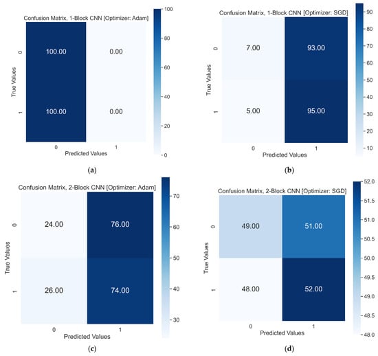
Figure 8.
Test Results in confusion matrix, 0 and 1 on x and y represent Healthy RBCs and SCs, respectively: (a) Confusion matrix of one-block CNN with Adam optimizer. (b) Confusion matrix of one-block CNN with SGD optimizer. (c) Confusion matrix of two-block CNN with Adam optimizer. (d) Confusion matrix of two-block CNN with SGD optimizer.
The loss and accuracy curves of three-block CNNs with SGD showed signs of overfitting, which means that the model may have performed poorly with the test dataset. It could be the reason for the decrease in the test accuracy score of the three-block CNN model with SGD from 50% to 48%. The f1 score of the model was below 50%, scoring precision values of 0.47 and 0.48 for healthy RBCs and SCs, respectively. Similarly, the three-block model with the Adam optimizer could not improve significantly, generating f1 scores of 0.33 and 0.60 for healthy RBCs and SCs, respectively. Figure 9 shows the confusion matrices of the three-block model with the Adam and SGD optimizers.
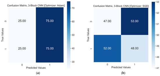
Figure 9.
Test results in a confusion matrix, 0 and 1 on x and y represent Healthy RBCs and SCs, respectively: (a) Confusion matrix of three-block CNN with Adam optimizer. (b) Confusion matrix of three-block CNN with SGD optimizer.
The use of Resnet50 andVGG16 as pre-trained models resulted in achieving higher validation accuracy in fewer epochs. The learning curves for both pre-trained models showed a good fit. When these models were tested on the test dataset, VGG16 showed the best performance with a test accuracy score of 98%. The confusion matrix in Figure 10 shows only three falsely classified images with the VGG16 model. On the other hand, Resnet50 could not perform better on the test dataset, showing accuracy scores of 65% and 64% with the Adam and SGD optimizers, respectively. The Resnet50 model performed better than the first three models, but the performance was not comparable to VGG16.
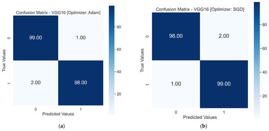
Figure 10.
Test results in a confusion matrix, 0 and 1 on x and y represent Healthy RBCs and SCs, respectively: (a) Confusion matrix of VGG16 with Adam optimizer. (b) Confusion matrix of VGG16 with SGD optimizer. (c) Confusion matrix of Resnet50 with Adam optimizer. (d) Confusion matrix of Resnet50 with SGD optimizer.
The test accuracies of all five models with both optimizers are compared in Figure 11. The first two models (with the SGD optimizer) achieved higher accuracy than models trained with the Adam optimizer. On the other hand, Adam performed better in the third and fifth models.
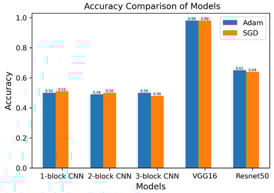
Figure 11.
Test accuracy comparison of models.
The accuracy scores of VGG16 and Resnet50 were higher than the accuracy scores of the first three models. The accuracy score reflects the total performance of the model but does not indicate the misclassified images from the testing dataset. The f1 score is a measure of incorrectly classified images from each class. The comparison of models based on f1 scores is shown in Figure 12. The f1 score is a function of the precision and recall scores of the model and becomes significant when false positives and false negatives are critical. For the classification of SCs, Adam performed better with the first, second and third models with higher f1 scores, and SGD performed better with the VGG16 and Resnet50 models.
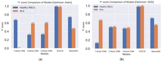
Figure 12.
f1 score comparison of models: (a) f1 score comparison of models with the Adam optimizer (b) f1 score comparison of models with the SGD optimizer.
Another way to illustrate the diagnostic ability of the binary classifier is by plotting the Receiver Operating Characteristic (ROC) curve, as shown in Figure 13. The increasing values on the x-axis indicate higher FPs than TNs; however, the higher values on the y-axis indicate more TPs than FNs. The comparison of both pre-trained models, VGG16 and Resnet50, is shown in Figure 13. VGG16 with both optimizers showed the highest values of TPs than FPs with the highest Area Under the Curve (AUC) value of 0.98. VGG16 performed better than the Resnet50 pre-trained model, as indicated in the study [58].
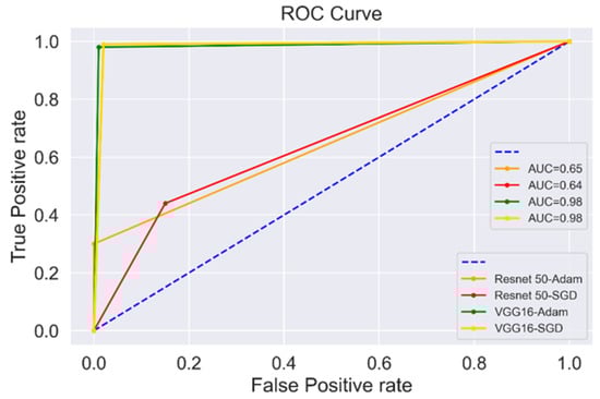
Figure 13.
ROC curve plot for VGG16 and Resnet50.
6. Conclusions
The use of DL algorithms in medical imaging has the prime purpose of predicting accurately to make judgments for a correct diagnosis. This study focused on designing a model to correctly classify microscopic blood samples, providing grounds for further research by biomedical researchers. This study included five DL models compiled dually with the Adam and SGD optimizers. The test accuracy scores of the first, second and third models, with both optimizers, could not surpass the value of 51%. However, for the classification of SCs, SGD performed better than Adam with the VGG16 and Resnet50 models. The use of VGG16 as a fourth model brought an exponential rise in accuracy, indicating a higher feature extraction ability and empowering the classifier to generalize better on the test dataset, with an accuracy of 98%. One limitation of this study is that the specific undisclosed dataset from the Lorrca Ektacytometry microscope was used for the training, validation and testing of the classifier. This study will be extended further to annotate sickle cells from the same undisclosed dataset to measure their deformability.
Author Contributions
Writing—original draft, M.B.; Writing—review & editing, A.d.K. All authors have read and agreed to the published version of the manuscript.
Funding
No external funding or grant was received.
Institutional Review Board Statement
Not applicable.
Informed Consent Statement
Not applicable.
Data Availability Statement
The dataset used in this study is not public or publicly archived.
Acknowledgments
The author, Marya Butt, thanks the Katrin Tazelaar, TechValley-NH, and the Research Director of R.R. Mechatronics, Jan de Zoeten, for providing support and valuable feedback.
Conflicts of Interest
The authors declare no conflict of interest.
References
- Abduljabbar, R.; Dia, H.; Liyanage, S.; Bagloee, S.A. Applications of Artificial Intelligence in Transport: An Overview. Sustainability 2019, 11, 189. [Google Scholar] [CrossRef]
- Makridakis, S.; Spiliotis, E.; Assimakopoulos, V. Statistical and Machine Learning forecasting methods: Concerns and ways forward. PLoS ONE 2018, 13, e0194889. [Google Scholar] [CrossRef] [PubMed]
- Latif, J.; Xiao, C.; Imran, A.; Tu, S. Medical Imaging using Machine Learning and Deep Learning Algorithms: A Review. In Proceedings of the 2019 2nd International Conference on Computing, Mathematics and Engineering Technologies (iCoMET), Sukkur, Pakistan, 10–13 June 2019; pp. 1–5. [Google Scholar] [CrossRef]
- Kersting, K. Machine Learning and Artificial Intelligence: Two Fellow Travelers on the Quest for Intelligent Behavior in Machines. Front. Big Data 2018, 1, 6. [Google Scholar] [CrossRef] [PubMed]
- Goodfellow, I.; Bengio, Y.; Courville, A. Deep Learning; MIT Press: Cambridge, MA, USA, 2016; Online. [Google Scholar]
- Nisbet, R.; Miner, G.; Yale, K. Chapter-19, Deep Learning. In Handbook of Statistical Analysis and Data Mining Applications, 2nd ed.; Academic Press: Boca Raton, NJ, USA, 2018. [Google Scholar]
- Chen, X.-W.; Lin, X. Big Data Deep Learning: Challenges and Perspectives. IEEE Access 2014, 2, 514–525. [Google Scholar] [CrossRef]
- Yu, Y.; Hur, T.; Jung, J.; Jang, I.G. Deep learning for determining a near-optimal topological design without any iteration. Struct. Multidiscip. Optim. 2018, 59, 787–799. [Google Scholar] [CrossRef]
- Dahl, G.E.; Yu, D.; Deng, L.; Acero, A. Context-Dependent Pre-Trained Deep Neural Networks for Large-Vocabulary Speech Recognition. IEEE Trans. Audio Speech Lang. Process. 2011, 20, 30–42. [Google Scholar] [CrossRef]
- Hinton, G.; Deng, L.; Yu, D.; Dahl, G.E.; Mohamed, A.-R.; Jaitly, N.; Senior, A.; Vanhoucke, V.; Nguyen, P.; Sainath, T.N.; et al. Deep Neural Networks for Acoustic Modeling in Speech Recognition: The Shared Views of Four Research Groups. IEEE Signal Process. Mag. 2012, 29, 82–97. [Google Scholar] [CrossRef]
- Cireşan, D.; Meler, U.; Cambardella, L.; Schmidhuber, J. Deep, big, simple neural nets for handwritten digit recognition. Neural Comput. 2010, 22, 3207–3220. [Google Scholar] [CrossRef]
- Zeiler, M.D.; Taylor, G.W.; Fergus, R. Adaptive deconvolutional networks for mid and high level feature learning. In Proceedings of the 2011 IEEE International Conference on Computer Vision, Barcelona, Spain, 6–13 November 2011; pp. 2018–2025. [Google Scholar] [CrossRef]
- Rahman Minar, M.; Naher, J. Recent Advances in Deep Learning: An Overview, CoRR, abs/1807.08169 (2018). Available online: http://arxiv.org/abs/1807.08169 (accessed on 20 November 2021).
- Turner, V.; Gantz, J.F.; Reinsel, D.; Minton, S. The digital universe of opportunities: Rich data and the increasing value of the internet of things. IDC Analyze Future 2014, 16, 13–19. [Google Scholar]
- Adnan, K.; Akbar, R.; Khor, S.W.; Ali, A.B.A. Role and Challenges of Unstructured Big Data in Healthcare. Data Manag. Anal. Innov. 2019, 20, 301–323. [Google Scholar] [CrossRef]
- Harrell, F.E., Jr.; Lee, K.L.; Matchar, D.B.; Reichert, T.A. Regression models for prognostic prediction: Advantages, problems, and suggested solutions. Cancer Treat. Rep. 1985, 69, 1071–1077. [Google Scholar] [PubMed]
- Pa, M.K.; Raja, S.S. Deep Learning Based Image Classification and Abnormalities Analysis of MRI Brain Images. In Proceedings of the 2019 TEQIP III Sponsored International Conference on Microwave Integrated Circuits, Photonics and Wireless Networks (IMICPW), Tiruchirappalli, India, 22–24 May 2019; pp. 427–431. [Google Scholar] [CrossRef]
- Anderson, K.M.; Odell, P.M.; Wilson, P.W.; Kannel, W.B. Cardiovascular disease risk profiles. Am. Hear. J. 1991, 121, 293–298. [Google Scholar] [CrossRef]
- Mondal, S.; Agarwal, K.; Rashid, M. Deep Learning Approach for Automatic Classification of X-Ray Images using Convolutional Neural Network. In Proceedings of the 2019 Fifth International Conference on Image Information Processing (ICIIP), Shimla, India, 15–17 November 2019; pp. 326–331. [Google Scholar] [CrossRef]
- Asri, H.; Mousannif, H.; Al Moatassime, H.; Noel, T. Using Machine Learning Algorithms for Breast Cancer Risk Prediction and Diagnosis. Procedia Comput. Sci. 2016, 83, 1064–1069. [Google Scholar] [CrossRef]
- Wheeless, L.L.; Robinson, R.D.; Lapets, O.P.; Cox, C.; Rubio, A.; Weintraub, M.; Benjamin, L.J. Classification of red blood cells as normal, sickle, or other abnormal, using a single image analysis feature. Cytometry 1994, 17, 159–166. [Google Scholar] [CrossRef]
- NIH. Sickle Cell Disease. Available online: https://ghr.nlm.nih.gov/condition/sickle-cell-disease#definition.
- Bush, A.M.; Borzage, M.T.; Choi, S.Y.; Václavů, L.; Tamrazi, B.; Nederveen, A.J.; Coates, T.D.; Wood, J.C. Determinants of resting cerebral blood flow in sickle cell disease. Am. J. Hematol. 2016, 91, 912–917. [Google Scholar] [CrossRef]
- Xin, M.; Wang, Y. Research on image classification model based on deep convolution neural network. EURASIP J. Image Video Process. 2019, 2019, 40. [Google Scholar] [CrossRef]
- Yao, Q.; Liao, X.; Jin, H. Training deep neural network on multiple GPUs with a model averaging method. Peer-to-Peer Netw. Appl. 2018, 11, 1012–1021. [Google Scholar] [CrossRef]
- Mohsen, H.; El-Dahshan, E.-S.A.; El-Horbaty, E.-S.M.; Salem, A.-B.M. Classification using deep learning neural networks for brain tumors. Futur. Comput. Inform. J. 2018, 3, 68–71. [Google Scholar] [CrossRef]
- Patil, D.N.; Khot, U.P. Image processing based abnormal blood cells detection. Int. J. Technical. Res. Appl. 2017, 31, 37–43. [Google Scholar]
- Maity, M.; Mungle, T.; Dhane, D.; Maiti, A.K.; Chakraborty, C. An Ensemble Rule Learning Approach for Automated Morphological Classification of Erythrocytes. J. Med. Syst. 2017, 41, 56. [Google Scholar] [CrossRef]
- Akrimi, J.A.; Suliman, A.; George, L.E.; Ahmad, A.R. Classification red blood cells using support vector machine. In Proceedings of the Information Technology and Multimedia (ICIMU), 2014 International Conference on IEEE, Putrajaya, Malaysia, 18–20 November 2014; pp. 265–269. [Google Scholar] [CrossRef]
- Rodrigues, L.F.; Naldi, M.C.; Maari, J.F. Morphological analysis and classification of erythrocytes in microscopy images. In Proceedings of the XII Workshop de Visao Computacional, Mato Grosso do Sul, Brazil, 9–11 November 2016; Volume 1, pp. 69–74. [Google Scholar]
- Samira; Veluchamy, M.; Perumal, K.; Ponnuchamy, T. Feature Extraction and Classification of Blood Cells Using Artificial Neural Network. Am. J. Appl. Sci. 2012, 9, 615–619. [Google Scholar] [CrossRef]
- Lotfi, M.; Nazari, B.; Sadri, S.; Sichani, N.K. The detection of Dacrocyte, Schistocyte and Elliptocyte cells in Iron Deficiency Anemia. In Proceedings of the Pattern Recognition and Image Analysis (IPRIA), 2015 2nd International Conference on IEEE, Rasht, Iran, 11–12 March 2015; pp. 1–5. [Google Scholar] [CrossRef]
- Elsalamony, H. Detection of some anaemia types in human blood smears using neural networks. Meas. Sci. Technol. 2016, 27, 085401. [Google Scholar] [CrossRef]
- Tomari, R.; Zakaria, W.N.W.; Jamil, M.M.A.; Nor, F.M.; Fuad, N.F.N. Computer Aided System for Red Blood Cell Classification in Blood Smear Image. Procedia Comput. Sci. 2014, 42, 206–213. [Google Scholar] [CrossRef]
- Poomcokrak, J.; Neatpisarnvanit, C. Red blood cells extraction and counting. In Proceedings of the 3rd International Symposium on Biomedical Engineering, Changsha, China, 8–10 June 2008; pp. 199–203. [Google Scholar]
- Abdulraheem Fadhel, M.; Humaidi, A.J.; Razzaq Oleiwi, S. Image processing-based diagnosis of sickle cell anemia in erythrocytes. In Proceedings of the 2017 Annual Conference on New Trends in Information & Communications Technology Applications (NTICT) IEEE, Baghdad, Iraq, 7–9 March 2017; pp. 203–207. [Google Scholar]
- Chy, T.S.; Rahaman, M.A. A Comparative Analysis by KNN, SVM & ELM Classification to Detect Sickle Cell Anemia. In Proceedings of the 2019 IEEE International Conference on Robotics, Electrical and Signal Processing Techniques (ICREST), Dhaka, Bangladesh, 10–12 January 2019; pp. 455–459. [Google Scholar]
- Alzubaidi, L.; Al-Shamma, O.; Fadhel, M.A.; Farhan, L.; Zhang, J. Classification of Red Blood Cells in Sickle Cell Anemia Using Deep Convolutional Neural Network. Adv. Intellig. Syst. Comput. 2019, 940, 550–559. [Google Scholar] [CrossRef]
- Xu, M.; Papageorgiou, D.P.; Abidi, S.Z.; Dao, M.; Zhao, H.; Karniadakis, G.E. A deep convolutional neural network for classification of red blood cells in sickle cell anemia. PLoS Comput. Biol. 2017, 13, e1005746. [Google Scholar] [CrossRef]
- Yao, X.; Sun, K.; Bu, X.; Zhao, C.; Jin, Y. Classification of white blood cells using weighted optimized deformable convolutional neural networks. Artif. Cells Nanomed. Biotechnol. 2021, 49, 147–155. [Google Scholar] [CrossRef]
- Rab, M.A.; Van Oirschot, B.A.; Bos, J.; Merkx, T.H.; Van Wesel, A.C.; Abdulmalik, O.; Safo, M.K.; Versluijs, B.A.; Houwing, M.E.; Cnossen, M.H.; et al. Rapid and reproducible characterization of sickling during automated deoxygenation in sickle cell disease patients. Am. J. Hematol. 2019, 94, 575–584. [Google Scholar] [CrossRef]
- Moolayil, J. An Introduction to Deep Learning and Keras. In Learn Keras for Deep Neural Networks; Apress: Berkeley, CA, USA, 2018; pp. 1–16. [Google Scholar] [CrossRef]
- Mikolajczyk, A.; Grochowski, M. Data augmentation for improving deep learning in image classification problem. In Proceedings of the International Interdisciplinary PhD Workshop (IIPhDW), Swinoujscie, Poland, 9–12 May 2018; pp. 117–122. [Google Scholar] [CrossRef]
- Engstrom, L.; Tran, B.; Tsipras, D.; Schmidt, L.; Madry, A. A rotation and a translation suffice: Fooling CNNs with simple transformations. arXiv 2017, arXiv:1712.02779. [Google Scholar]
- Shpilman, A.; Boikiy, D.; Polyakova, M.; Kudenko, D.; Burakov, A.; Nadezhdina, E. Deep Learning of Cell Classification Using Microscope Images of Intracellular Microtubule Networks. In Proceedings of the 16th IEEE International Conference on Machine Learning and Applications (ICMLA), Cancun, Mexico, 18–21 December 2017; pp. 1–6. [Google Scholar] [CrossRef]
- Kumar, V.; Singh, D.; Kaur, M.; Damaševičius, R. Overview of current state of research on the application of artificial intelligence techniques for COVID-19. PeerJ Comput. Sci. 2021, 7, e564. [Google Scholar] [CrossRef]
- Yamashita, R.; Nishio, M.; Do, R.K.G.; Togashi, K. Convolutional neural networks: An overview and application in radiology. Insights Imag. 2018, 9, 611–629. [Google Scholar] [CrossRef]
- Yang, X.; Ye, Y.; Li, X.; Lau, R.Y.K.; Zhang, X.; Huang, X. Hyperspectral Image Classification with Deep Learning Models. IEEE Trans. Geosci. Remote Sens. 2018, 56, 5408–5423. [Google Scholar] [CrossRef]
- Nirthika, R.; Manivannan, S.; Ramanan, A.; Wang, R. Pooling in convolutional neural networks for medical image analysis: A survey and an empirical study. Neural Comput. Appl. 2022, 34, 5321–5347. [Google Scholar] [CrossRef]
- Simonyan, K.; Zisserman, A. Very deep convolutional networks for large-scale image recognition. In Proceedings of the International Conference on Learning Representations, San Diego, CA, USA, 7–9 April 2014; pp. 1409–1556. [Google Scholar]
- He, K.M.; Zhang, X.Y.; Ren, S.Q.; ve Sun, J. Deep residual learning for image recognition. In Proceedings of the IEEE Conference on Computer Vision and Pattern Recognition, Las Vegas, NV, USA, 27–30 June 2016; pp. 770–778. [Google Scholar]
- Amir, A.; Butt, M.; Van Kooten, O. Using Machine Learning Algorithms to Forecast the Sap Flow of Cherry Tomatoes in a Greenhouse. IEEE Access 2021, 9, 154183–154193. [Google Scholar] [CrossRef]
- Chen, Y.; Qin, S.; Qiao, S.; Dou, Q.; Che, W.; Su, G.; Yao, J.; Nnanwuba, U.E. Spatial Predictions of Debris Flow Susceptibility Mapping Using Convolutional Neural Networks in Jilin Province, China. Water 2020, 12, 2079. [Google Scholar] [CrossRef]
- Taqi, A.M.; Awad, A.; Al-Azzo, F.; Milanova, M. The Impact of Multi-Optimizers and Data Augmentation on TensorFlow Convolutional Neural Network Performance. In Proceedings of the 2018 IEEE Conference on Multimedia Information Processing and Retrieval (MIPR), Miami, FL, USA, 10–12 April 2018; pp. 140–145. [Google Scholar] [CrossRef]
- Bera, S.; Shrivastava, V.K. Analysis of various optimizers on deep convolutional neural network model in the application of hyperspectral remote sensing image classification. Int. J. Remote Sens. 2019, 41, 2664–2683. [Google Scholar] [CrossRef]
- Jabbar, H.K.; Khan, D.R.Z. Methods to avoid over-fitting and under-fitting in supervised machine learning (comparative study). In Computer Science, Communication & Instrumentation Devices; Research Publishing Services: Singapore, 2014; pp. 163–172. [Google Scholar]
- Hardt, M.; Recht, B.; Singer, Y. Train faster, generalize better: Stability of stochastic gradient descent. In Proceedings of the International Conference on Machine Learning, New York, NY, USA, 20–22 June 2016; pp. 1225–1234. [Google Scholar]
- Vatathanavaro, S.; Tungjitnob, S.; Pasupa, K. White blood cell classification: A comparison between VGG-16 and ResNet-50 models. In Proceedings of the 6th Joint Symposium on Computational Intelligence, Seville, Spain, 18–20 August 2018; Volume 12, pp. 4–5. [Google Scholar]
Publisher’s Note: MDPI stays neutral with regard to jurisdictional claims in published maps and institutional affiliations. |
© 2022 by the authors. Licensee MDPI, Basel, Switzerland. This article is an open access article distributed under the terms and conditions of the Creative Commons Attribution (CC BY) license (https://creativecommons.org/licenses/by/4.0/).