HAGDAVS: Height-Augmented Geo-Located Dataset for Detection and Semantic Segmentation of Vehicles in Drone Aerial Orthomosaics

Abstract

Detection and Semantic Segmentation of vehicles in drone aerial orthomosaics has applications in a variety of fields such as security, traffic and parking management, urban planning, logistics, and transportation, among many others. This paper presents the HAGDAVS dataset fusing RGB spectral channel and Digital Surface Model DSM for the detection and segmentation of vehicles from aerial drone images, including three vehicle classes: cars, motorcycles, and ghosts (motorcycle or car). We supply DSM as an additional variable to be included in deep learning and computer vision models to increase its accuracy. RGB orthomosaic, RG-DSM fusion, and multi-label mask are provided in Tag Image File Format. Geo-located vehicle bounding boxes are provided in GeoJSON vector format. We also describes the acquisition of drone data, the derived products, and the workflow to produce the dataset. Researchers would benefit from using the proposed dataset to improve results in the case of vehicle occlusion, geo-location, and the need for cleaning ghost vehicles. As far as we know, this is the first openly available dataset for vehicle detection and segmentation, comprising RG-DSM drone data fusion and different color masks for motorcycles, cars, and ghosts.

Dataset:https://doi.org/10.5281/zenodo.6323712.

Dataset License: Licensed under Creative Commons Attribution 4.0 International.

1. Summary

Vehicle Detection and Semantic Segmentation are widely studied areas in computer vision and Artificial Intelligence; driverless cars are good evidence of this. Due to the rapid development, ease of acquisition, and low cost of drone aerial imagery [1], it is also becoming important to detect and segment vehicles in orthomosaics. However, deep learning models applied in this field still need to solve challenges, such as the following:

• Orthomosaics are geo-located and have a larger number of pixels compared to ground imagery [2].
• Vehicles have different shapes, colors, sizes, and textures [3].
• Spatial relations between vehicles and their surroundings are complex: densely-parked, occluded by trees or buildings, and heading in different directions [4,5,6].

Figure 1 illustrates the aforementioned challenges.

Research studies have used and released publicly available datasets for vehicle detection, which consist of bounding boxes (BBs) [2,3,4,5,6]. Horizontal BBs were used for different types of objects [7], and a dataset using horizontal BBs for cars was created by [7,8]. CARPK dataset [6] proposed the use of rotated BBs, improving previous results [6]. Figure 2 shows illustrations of horizontal and rotated BBs; in those datasets, cars are annotated in oblique drone images.

Segmentation datasets of vehicles comprise binary image-masks, commonly obtained from satellites [2,9] and more recently from drones [10,11]. They constitute the base for training segmentation models, where pixel-level classification is performed and the U-Net architecture dominates [12]. A dataset consisting of images and their masks, coupled at the pixel level, is called a paired dataset [13]. Examples of other fields of research which employ paired datasets are facades, shoes, handbags, maps, and cityscapes [14]. Las Vegas, SpaceNet, DeepGlobe, and Potsdam-Vaihingen datasets [2,12,14,15,16,17,18] are good examples of detection and segmentation datasets created using satellite imagery. The research study [19] proposed the use of line segments to annotate boat length and heading direction using DigitalGlobe satellite imagery. The Stanford Drone Dataset (SDD) [4,20] and the VisDrone2021 dataset [11,21] are video and oblique imagery for real-time object detection. DroneDeploy dataset [10] is obtained from drone orthomosaics; it contains separate DSM files [22] and segmentation masks for different objects to create landcover maps. DroneDeploy dataset is considered imbalanced with respect to the ground class [10]. Figure 3 illustrates one example of image and mask of the Potsdam’s satellite dataset [23].

Deep Learning Models’ robustness and accuracy depend on their learning from the training data. Therefore, it is necessary to include variations in data and new information for the model to better recognize the unknown data [24]. In [15], it was shown that using additional information to the RGB satellite images, specifically the infrared band, improved vegetation and building segmentation results. In [22], it was investigated how RGB plus DSM information, obtained from UAV, improved the semantic segmentation of multi-classes in landcover maps.

To help the deep learning community, we propose the HAGDAVS dataset, which consists of vector bounding boxes and segmentation masks for motorcycles, cars, and ghosts of vehicles. The two main outstanding characteristics of the proposed dataset are as follows:

• The fusion of height information of vehicles in one channel of the image. This aims to help with segmenting vehicles of surrounding objects such as buildings and roads, and perhaps enhancing model behavior in the case of shadows or partial occlusions affect vehicle segmentation.
• Inclusion of ghost class. This dataset becomes the first in this category, which serves the purpose of creating applications to improve orthomosaic quality and visualization.

The proposed dataset is described in the next section.

2. HAGDAVS Dataset Description

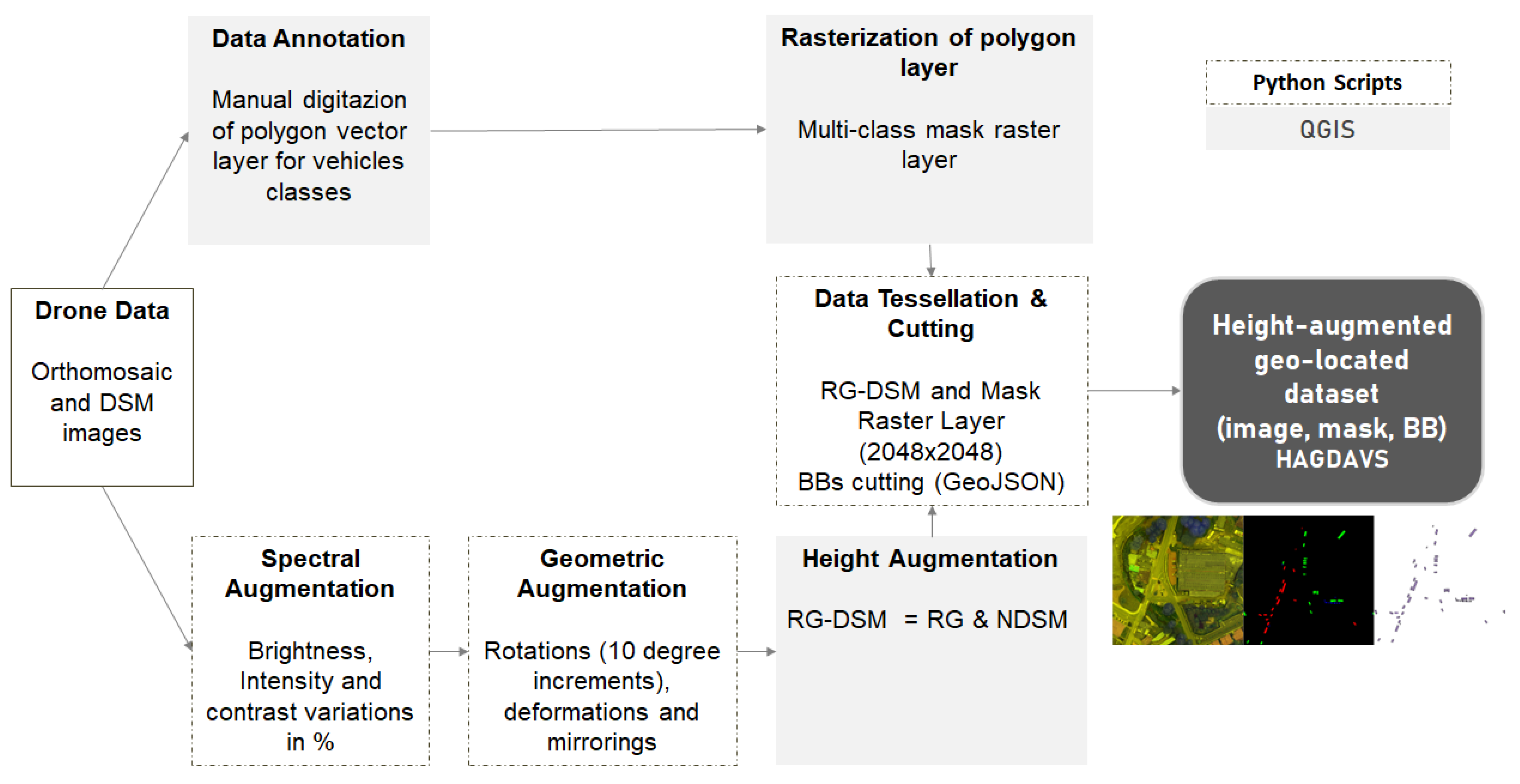
HAGDAVS dataset is obtained by the fusion of RG channels, from RGB high resolution drone orthomosaics, with the DSM 1-channel image to obtain an RG-DSM image. Height-augmentation of images aids in classifying pixels of vehicles, especially when their spectral responses are similar to those of a vehicle’s surroundings. For detection of vehicles, bounding boxes are drawn manually over geo-located orthomosaics, and provided in GeoJSON vector opensource format [25]. This allows us to geo-locate vehicles as well. For segmentation, RG-DSM images are spatially paired pixel by pixel with color mask images that represent three classes: class 1 for motorcycles, class 2 for cars of any type, and class 3 for any undesired ghost object of the two previous classes.

Orthomosaics are created by stitching images that partially overlap, using a method called Structure from Motion (SfM) [26]. Ghosts are formed when objects present in a scene are not in the same position in the overlapping images [27]. This makes ghosts common for moving objects, as they shift position between one image and the corresponding overlapping images of a specific scene. Removing the ghost effect is a manual process in which the user has to edit the mosaic in a proprietary software [26], drawing a region around the vehicle and selecting an image in which the moving object does not appear [26]. To improve an orthomosaic, this process has to be followed for every existing ghost. However, there are studies on performing this process automatically with the aid of computer vision [28]. Class 3 supports the creation of AI-based image cleaning algorithms, or removal of false positives caused by moving vehicles [19,29]. Finally, class 0 is the background, represented by black color. The proposed dataset aims to improve model generalization and robustness by including diverse examples of vehicles and their classes, occlusions caused by buildings or trees, and the unwanted ghosts of motorcycles and cars.

Table 1. Orthomosaic and DSM characteristics, and the number of examples per class.

Orthomosaics	DSM	Class 1 (Motorcycle)	Class 2 (Car)	Class 3 (Ghost)	Total
El Retiro Cols, Rows: 8721, 15,332 GSD 7.09, Size: 510.1 MB Format: TIFF, Bands: 3 Pixel Depth: 8 Bit Spatial Reference: GCS_WGS1984	Height-Range: 2169–2314 m Xmin,Ymin (−755,057,859, 60,534,441) Xmax,Ymax (−754,977,854, 60,654,446)	209 examples	527 examples	94 examples	830 examples
La Ceja Cols, Rows: 8361, 5375 GSD 5.51, Size: 171.4 MB Format: TIFF, Bands: 3 Pixel Depth: 8 Bit Spatial Reference: GCS_WGS1984	Height-Range: 2158–2214 m Xmin,Ymin (−754,379,007, 60,342,695) Xmax,Ymax (−754,332,962, 60,313,098)	47 examples	120 examples	71 examples	238 examples
Rionegro Cols, Rows: 8847, 18,895 GSD 6.08, Size: 637.7 MB Format: TIFF, Bands: 3 Pixel Depth: 8 Bit Spatial Reference: GCS_WGS1984	Height-Range: 2065–2135 m Xmin,Ymin (−753,809,074, 61,394,740) Xmax,Ymax (−753,760,197, 614,98,805)	271 examples	1051 examples	321 examples	1643 examples
Pradolargo Cols, Rows: 14,919, 6666 GSD 6.30, Size: 379.4 MB Format: TIFF, Bands: 3 Pixel Depth: 8 Bit Spatial Reference: GCS_WGS1984	Height-Range: 2493–2605 m	12 examples	32 examples	104 examples	148 examples
	Xmin,Ymin (−755,311,888, 61,563,654) Xmax,Ymax (−755,226,877, 61,601,860)
TOTAL		539	1730	590	2859

describes orthomosaic characteristics and summarizes the total number of examples per class and orthomosaic. Figure 4 shows examples of images and multi-class masks of our paired dataset.

The dataset is comprised of five folders, with one for the RG-DSM images, one for the multi-color image masks, and one for the bounding boxes. The other two are for RGB and DSM images. These last two folders are in case researchers want to test the benefit of using height in models, with respect to RGB-only or DMS-only images. Every image folder has 83 paired images of 2048 × 2048 pixels in TIFF format, 8 bit, and three channels, except for the DSM. An RG-DSM image contains red and green colors in the first two channels and Digital Surface Model’s height in the third channel [30]. Images are numbered in ascending order.

Table 2. The HAGDAVS dataset specifications.

Item	Description
Field of application	Vehicle detection or segmentation
Collected data	Aerial images
Method for data acquisition	Drone flights
Used drone	DJI Phantom 4 Pro V2
Camera resolution and sensor size	20Mpx, 1 inch CMOS
Software for processing of collected data and products	Opendronemap [1], Orthomosaics and DSM
GSD of obtained orthomosaics and DSM	5.5 to 7.1 cm/px
Method of annotation	Manually in GIS and semi-automated via Python scripts
Dataset production	GDAL scripts in Jupyter Notebook
Language for scripts	Python 3.7
Used GIS software	QGIS V3.22.2-Białowieża, ArcGIS
Number of classes and objects	4: motorcycle, car, and ghost (motorcycle or car), background
Number of orthomosaics	4
Data collected by	Authors of this paper
Year of collection	2018–2020
Detection dataset	GeoJSON bounding boxes
Segmentation dataset	RG-NDSM 1, Multi-class color mask images
Additional information	RGB, DSM
Dataset size	1.34 Gb compressed
Image format	.tiff
Image quantity	83 images
Cols, Rows of images	2048 × 2048 px
RGB, RG-DSM1 Image average memory size	16 Mb
RGB, RG-DSM1, Mask, Image spectral resolution	3 bands
RGB, RG-DSM, Mask Image radiometric resolution	8 bit
RGB, RG-DSM, Mask Image Coordinate System	WGS1984

¹ Inclusion of DSM’s height in an RGB image.

summarizes our dataset specifications.

3. Methods

Aerial imagery, especially drone orthomosaics, is becoming ubiquitous. Ease of use and affordable price of consumer and professional drones are making this happen, rapidly increasing its availability and quality [4]. Methods applied to acquire and process drone data to produce the HAGDAVS dataset are presented in the next section.

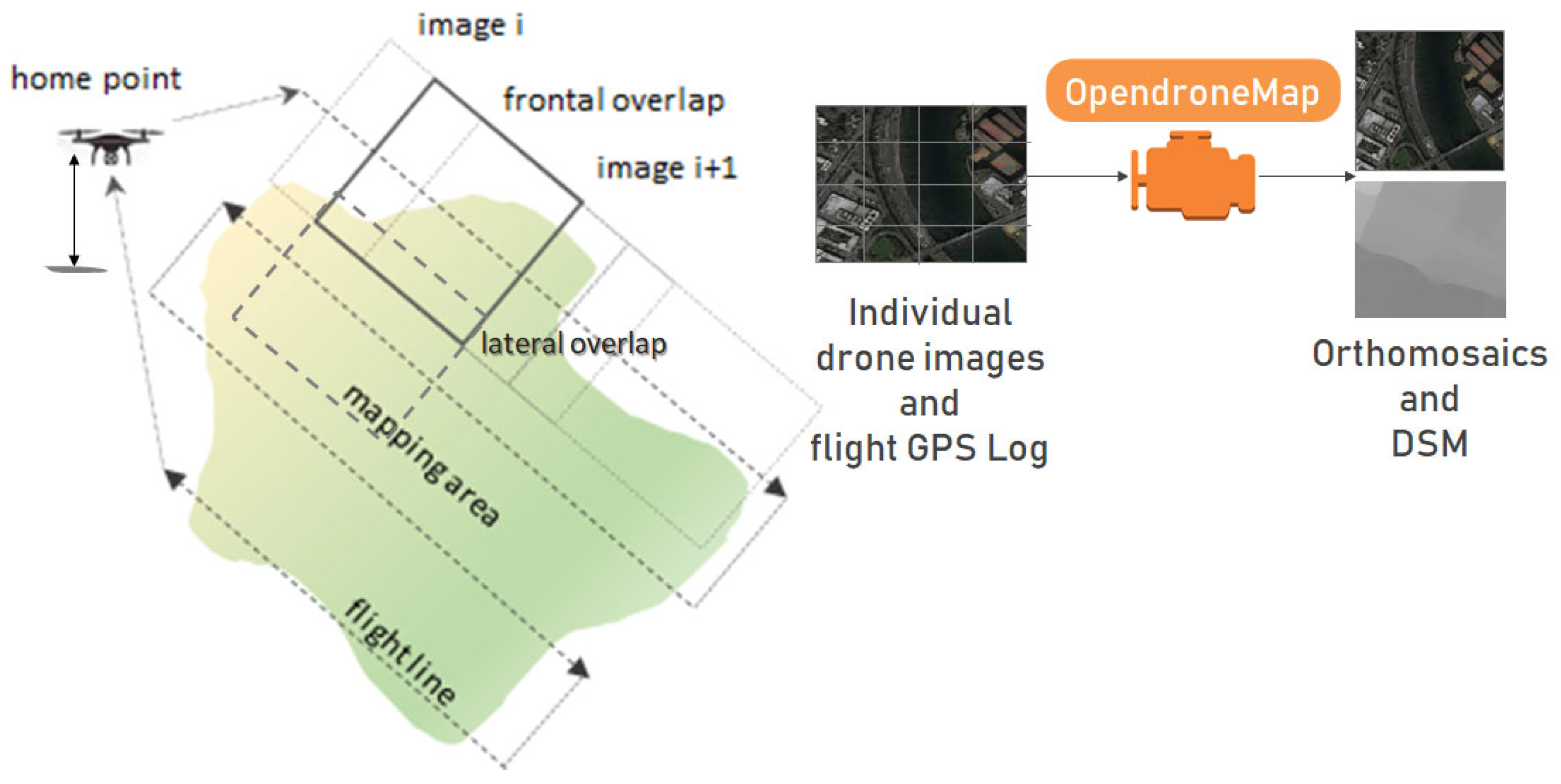
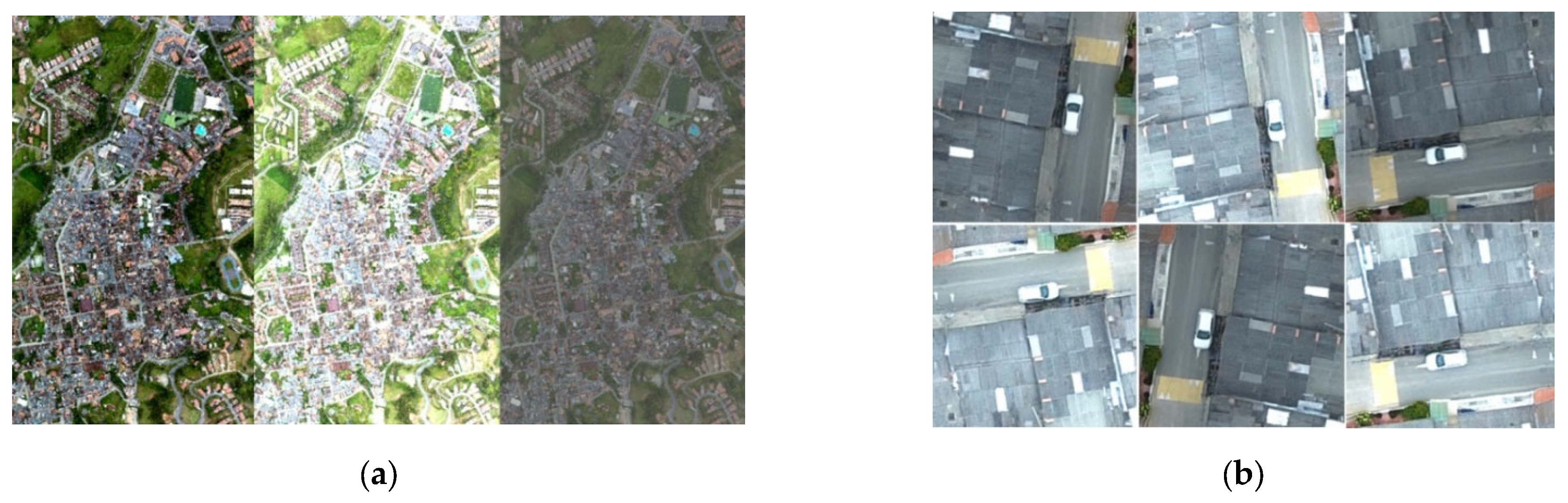
3.1. Data Acquisition and Processing

Data was acquired by executing several autonomous flights, using a drone Dji Phantom 4Pro V2 and the Capture App [31]. Four small urban areas, located in Colombia, South America, were photographed at heights between 100 and 150 m above ground level (AGL). Mapping areas were covered with flight lines using a frontal overlap of 85% and a lateral overlap of 75%. Individual images and GPS Log obtained during the flights were processed in Open Drone Map [32], an open-source software, to produce the orthomosaics, the DSM, and a 3D point cloud of every mapping area. These three are the most representative products when processing drone images [1]. The WGS1984 is the Geographical Coordinate System chosen for the products. Figure 5, illustrates the workflow for the acquisition and processing of individual images to obtain orthomosaics, DSM, and 3D point cloud.

Drone orthomosaics have a very high spatial resolution, measured by the Ground Sample Distance (GSD) [10,15,33,34], which is the physical pixel size; a 10 cm GSD means that each pixel in the image has a spatial extent of 10 cm. The GSD of an orthomosaic depends on the altitude of the flight (AGL). Figure 6 shows a snapshot of one of the obtained orthomosaics and corresponding DSM.

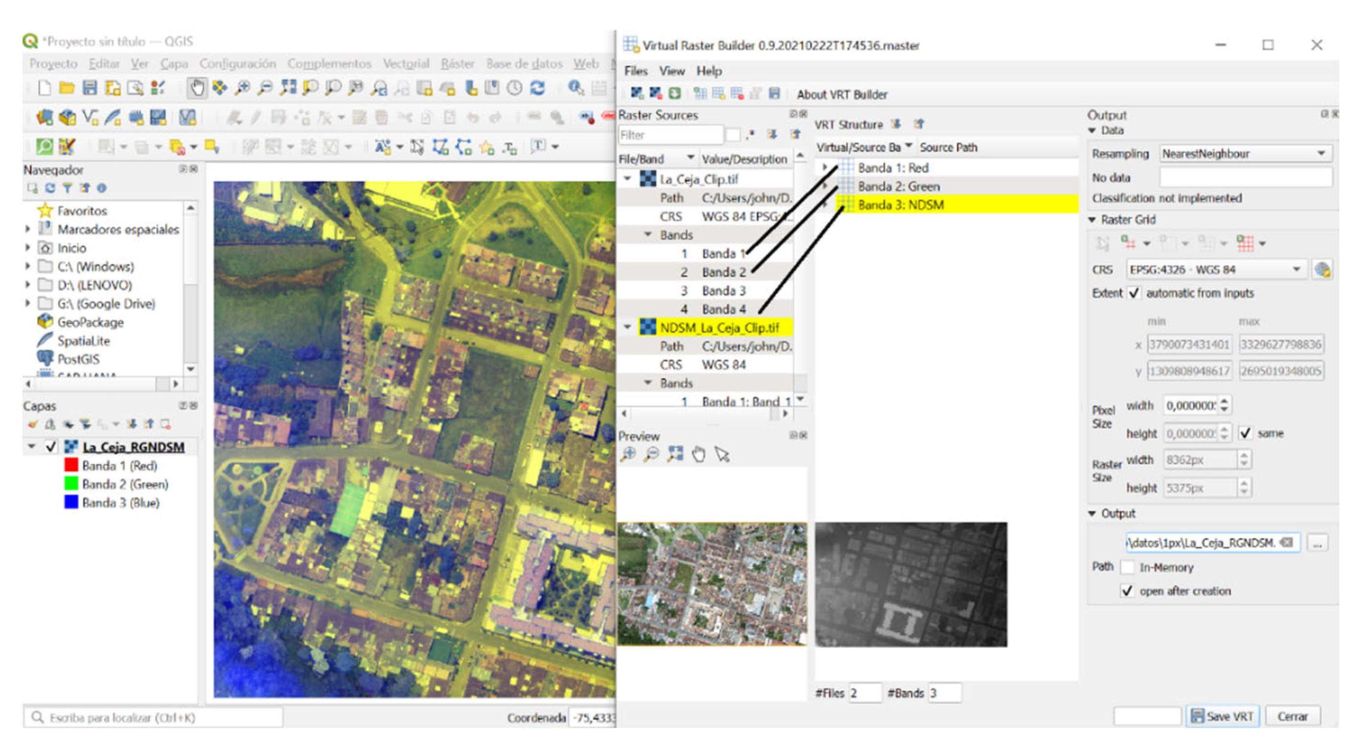
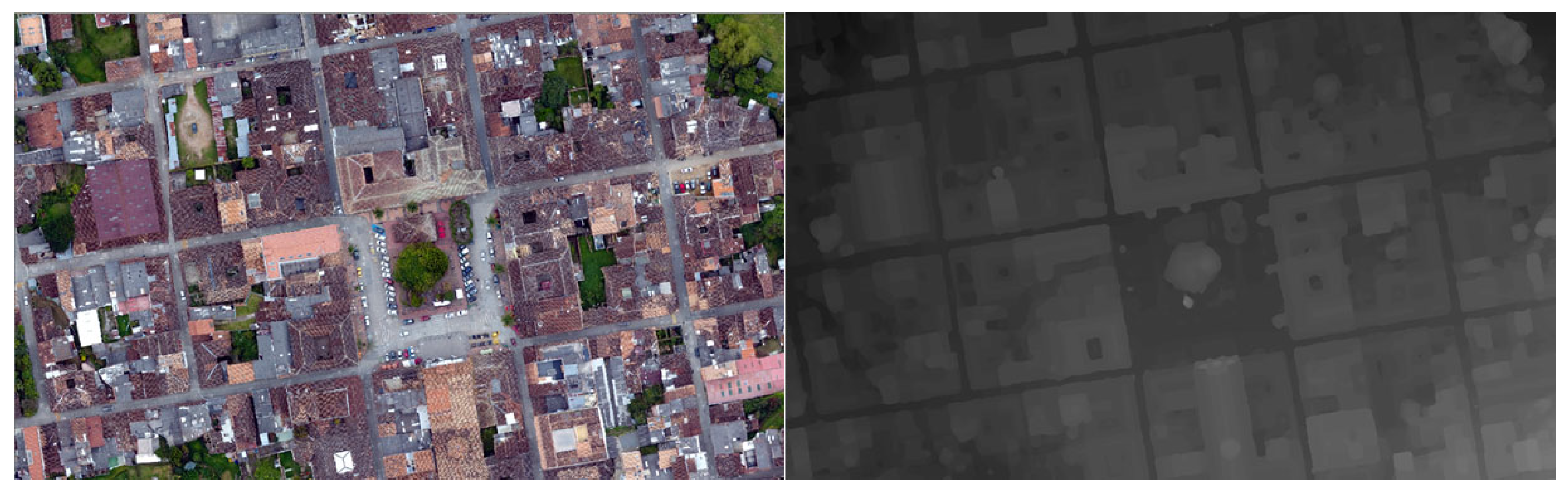
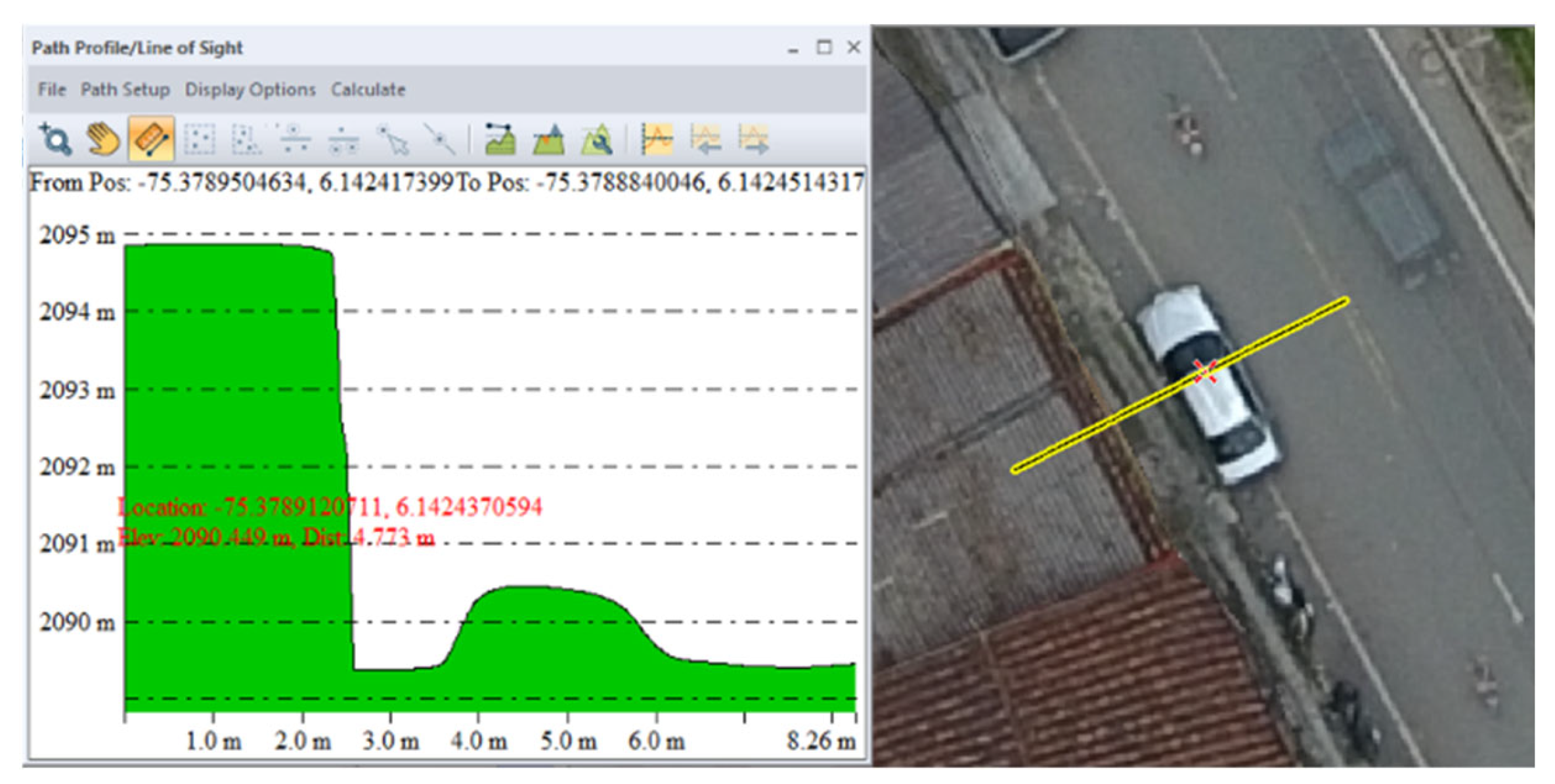
3.2. Height Augmentation

Due to computational restrictions, deep learning models commonly use RGB three channel images [10,11,12,13,14,16,17,35,36,37,38] and this is also the case for image datasets [2,9,10,18,20]. This situation may limit model generalization in the case of similarities of spectral response between neighbor objects, for instance, between vehicles and buildings, vehicles and trees, or vehicles and roads. The proposed dataset comprises red and green; instead of the blue channel, which is removed, we use height values of the DSM. Figure 7 shows the height value profile of the DSM in an urban scene.

The RG-DSM is a false color composite image [15,22,23,30], bluish in terms of objects’ height; the more blue the image, the higher the objects in the image. Height values may segment objects when spectral information is not enough [15]. Since RGB values are in range (0, 255), DMS height values should be rescaled to the interval (0, 255); this is called the NDSM, and it is calculated as follows:

$$\mathrm{NDSM}=255\ast \left(\mathrm{DSM}-\mathrm{minHeight}\right)/\left(\mathrm{maxHeight}-\mathrm{minHeight}\right)$$

(1)

where DSM is the Digital Surface Model (in meters), which has the same extension and GSD of the corresponding orthomosaic; and minHeight and maxHeight are the minimum and maximum height values (in meters) of the DSM, respectively. Figure 8 shows the tool used in QGIS to obtain the RG-NDSM false color composite. The Virtual Raster Builder tool allows us to combine raster bands by dragging them in an appropriate order.

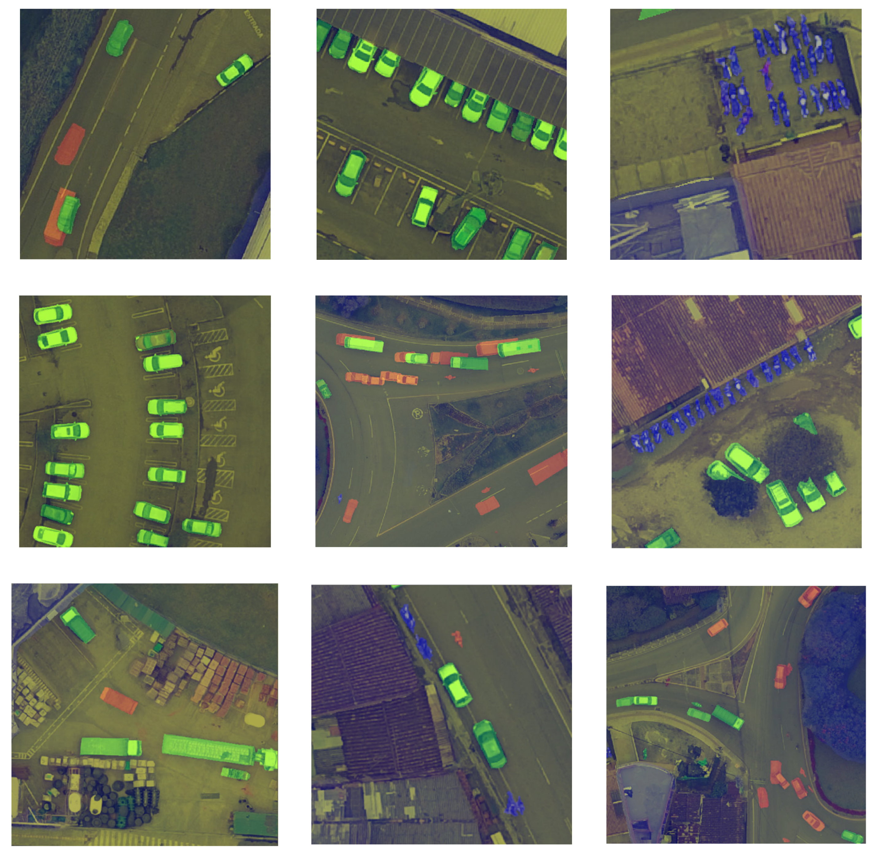
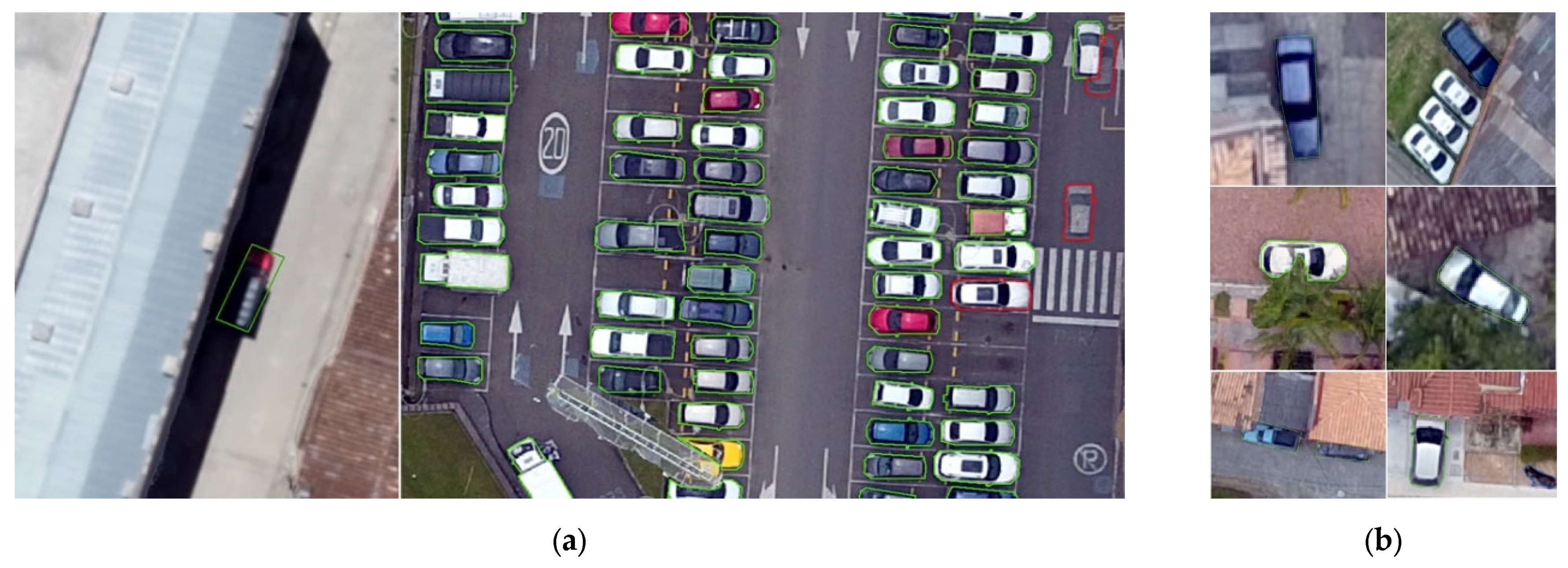
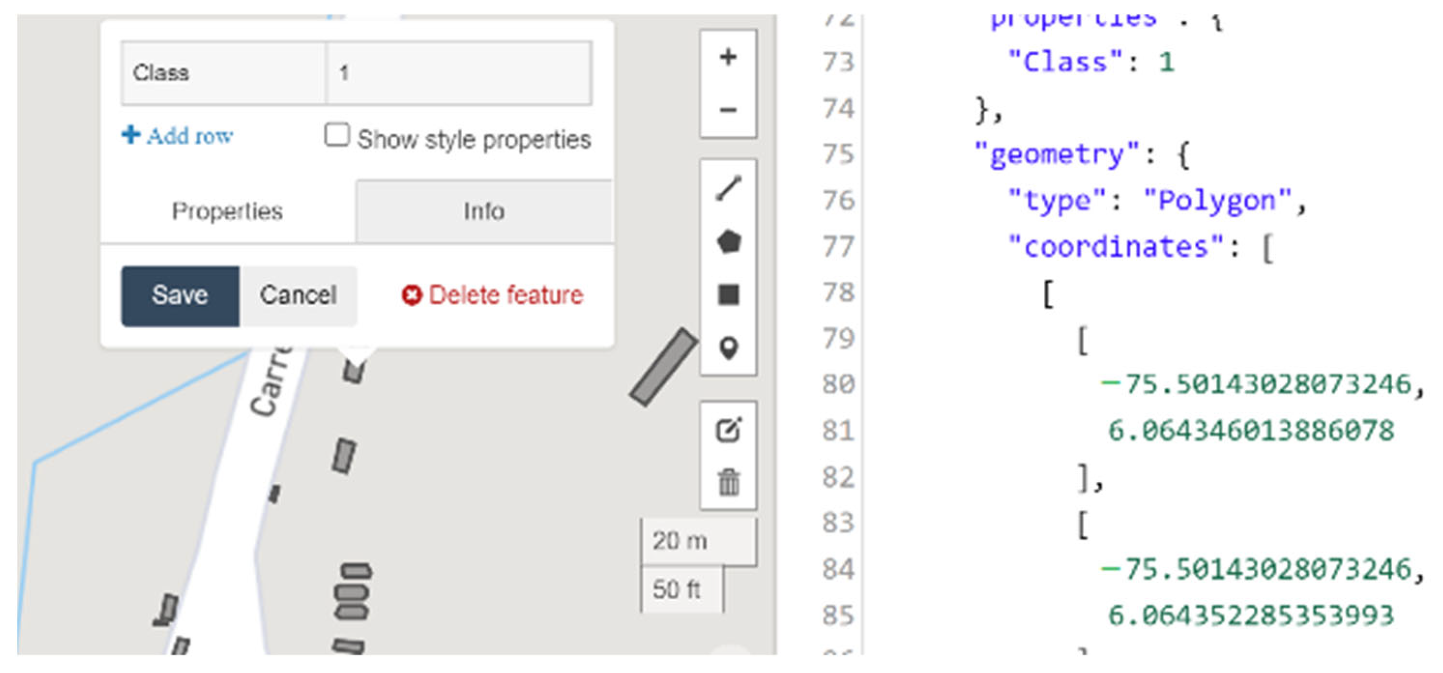
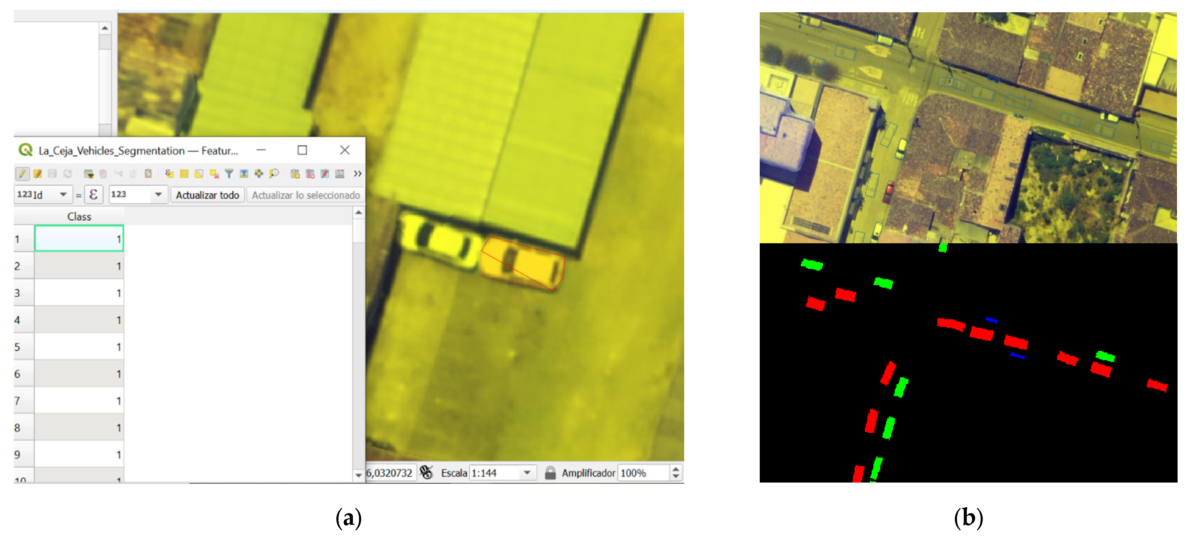
3.3. Data Annotation and Data Curation

Initially, the three types of vehicles in the dataset (motorcycles, cars, and ghosts) are digitized on the screen over each orthomosaic as a base layer. This was done in the QGIS open-source software [37], obtaining a polygon GIS layer in shapefile format (*.shp). An integer field called “Class” was created in the shapefile to distinguish the type of vehicle, with values as follows: 1 for motorcycles, 2 for cars, and 3 for ghosts. Digitation zoom is between 1:40 and 1:80 for all the orthomosaics, to ensure capture of details. This task is time consuming, but it is the base for obtaining detection bounding boxes and multi-class masks for segmentation. Figure 9 shows resulting bounding boxes in GeoJSON format [25]. Figure 10 illustrates the data annotation process.

The polygon shapefile of each orthomosaic is converted to GeoJSON vector format using a script in Python. Every GeoJSON file has the same extension and spatial reference system of the corresponding orthomosaic. At the same time, a multi-class mask raster layer is created for each orthomosaic by rasterizing every polygon shapefile, using the “Class” field, including the background as an extra class (class 0). It is exported in Tiff format with 8-bit radiometric resolution. Resultant images have the same spatial reference and extension of the corresponding orthomosaic. In a mask raster layer, red pixels represent ghost objects, green pixels represent cars, blue pixels represent motorcycles, and black color pixels represent the background.

The dataset has been curated in terms of exhaustive revision of images to avoid violation of privacy and affectation of third parties.

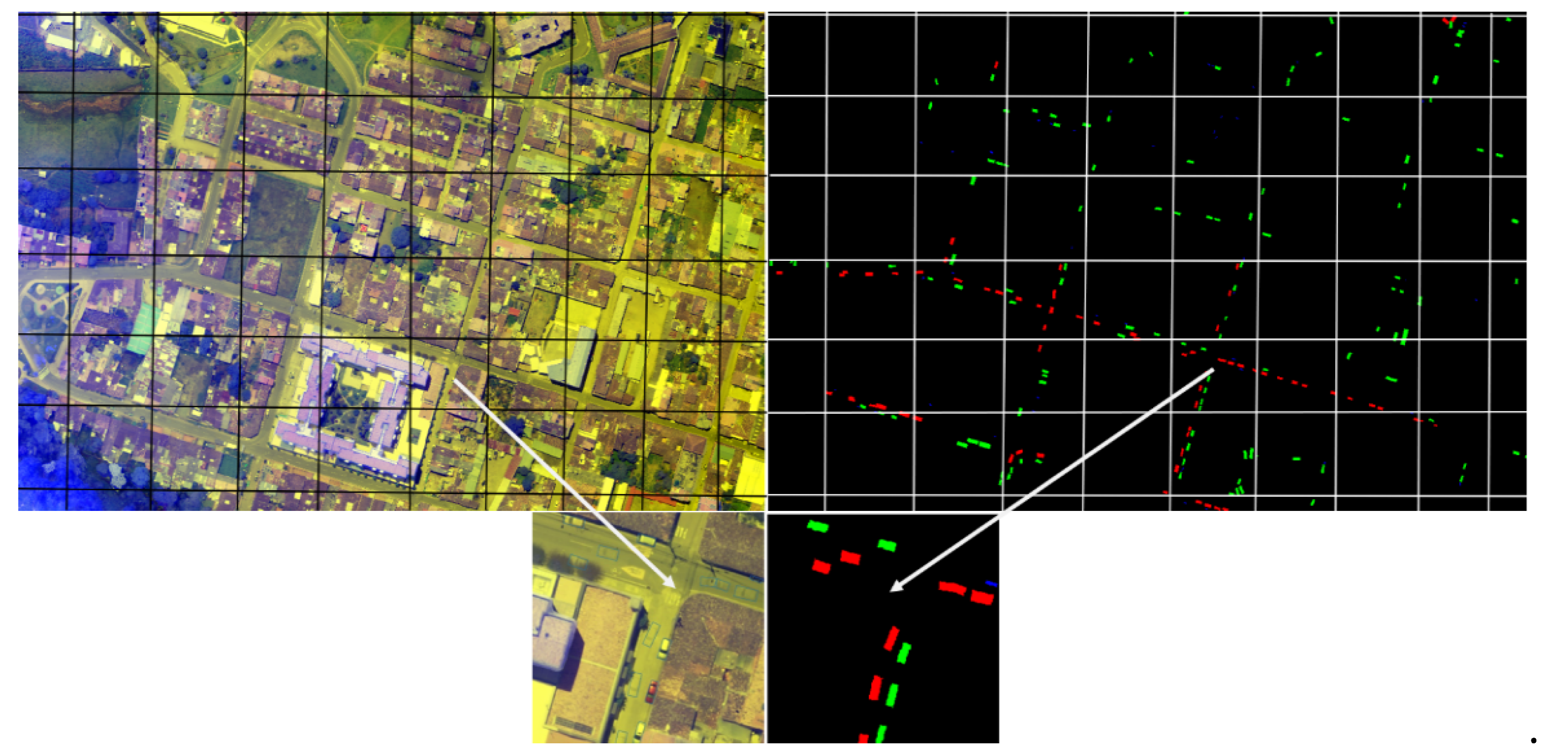
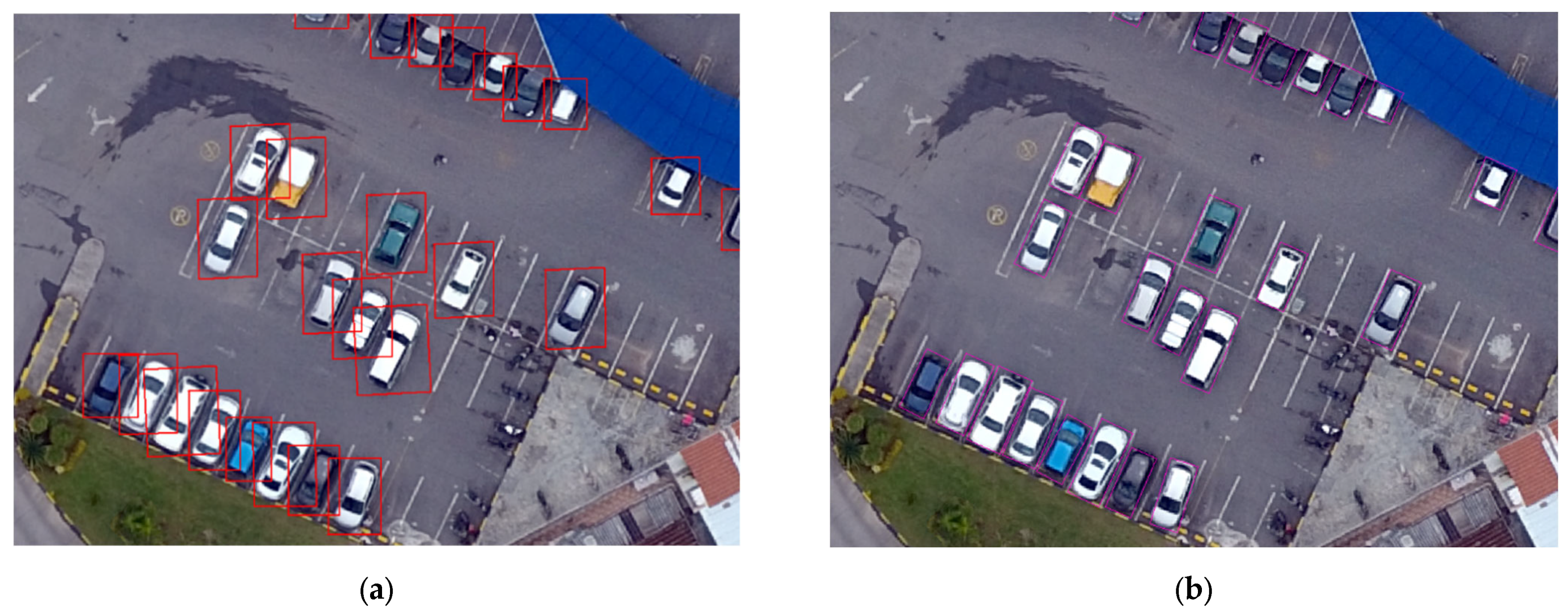
3.4. Data Tessellation and Cutting

Every RG-NDSM and corresponding mask raster layer (four in total) is tessellated into 2048 × 2048-pixel Tiff images, and saved in two separate folders (RG-NDSM, Masks). Tessellation was made using a GDAL-OGR python script that keeps spatial reference. RGB and DSM are also tessellated and saved in folders (RGB, DSM) following the same procedure. All corresponding images are named with integer numbers in ascending order. Images without multi-color vehicle masks (completely black) or with dimensions less than 2048 × 2048 pixels are deleted in all folders. Bounding boxes are obtained by cutting GeoJSON files for each orthomosaic with the same size of tessellated RG-DSM or Masks; these files are saved in the BBs folder using Python script. Jupyter Notebook Scripts (*.ipynb) can be downloaded from the GitHub directory of this paper (https://github.com/jrballesteros/Vehicle_extraction_Dataset accessed on 8 March 2022). Figure 11 shows the tessellation process for RG-DSM and mask images. Figure 12 shows the complete workflow to obtain the proposed dataset.

3.5. Dataset Bias

In general, computer vision, as well as digital image analysis, tend to be fields with a high degree of data imbalance. Within an image, only a portion of it corresponds to the feature of interest; this is the positive class. The rest of the image is usually assigned to another category or negative class, although there are also several other classes. This simple but convenient way of labeling images is often the biggest cause of imbalanced dataset generation. The acquisition process, the device used, and the illumination limitations among others constitute additional causes for imbalanced image dataset generation [38]. This class imbalance within a dataset is called dataset bias.

Models trained with imbalanced datasets may be affected by the dataset bias. Many techniques are proposed to face this problem. Resampling techniques are the most traditional approach. Over-sampling the minor class, under-sampling the majority class, or combining over- and under-sampling belong to this category. However, recent techniques seem to help resolve this problem in a more convenient way, for example, data augmentation, adequate data split, and the design of optimization functions that allow the inclusion of weights for each class, penalizing according to the number of samples in the dataset.

In HAGDAVS, the number of samples by class are shown in Table 1. The Background Class has significantly more information than the other classes. Additionally, sample differences between vehicle classes are also present. The Car class has around three times more samples than the Motorcycle and Ghost classes. We suggest the following techniques to mitigate the class imbalance problem in the proposed dataset.

3.5.1. Data Augmentation and Splitting

Data augmentation tends to improve model generalization [2,10,19,23,24], increasing the number of available examples to train a model. Two other types of data augmentation may be applied to the dataset before training a model or during the training: spectral and geometric augmentation [24]. Spectral refers to the change in contrast, intensity, or brightness of images [24]. Values of 25% above and below normal contrast and brightness may be used. The intensity or gamma value improves contrast in dark or highly illuminated parts of images [39]. Geometric augmentation refers to rotations, zooming, and deformation of images. Images and corresponding image masks can be rotated clockwise in 10-degree increments [19]. Vertical and horizontal mirroring is a transformation in which upper and lower, or right and left, parts of images interchange position [24]. In some cases, geometric augmentation improves a model’s metric performance more than spectral augmentation [1]. Figure 13 shows some examples of spectral and geometric data augmentation.

Since the HAGDAVS dataset has not been augmented or split, researchers can use any previously described procedure to increase the number of examples, or apply a specialized library to do it [24]. Researchers may also randomly split the dataset or use a special technique that, for instance, guarantees the number of vehicles per training image.

3.5.2. Data Imbalance and Sample Weights

In deep learning algorithms, sample weights in the loss or optimization functions can be introduced. The weight class is estimated according to its distributions in the dataset. For the loss functions, a larger weight is assigned to the samples belonging to the minor class; conversely, lower weights are assigned to the samples of the dominant class. In order to calculate the class weights, we suggest the Median Frequency Balancing approach, which is formulated in (2).

$${\alpha }_c=median\_freq/freq\left(c\right)$$

(2)

where ${\alpha }_c$ is the weight for all samples of the c class, $median\_freq$ is the median of the calculated frequencies for all classes, and$freq\left(c\right)$ is the total number of pixels of class c divided by the total number of pixels in the dataset.

3.6. Practical Applications of the HAGDAVS Dataset

The proposed dataset has the following practical applications:

• Detecting and enumerating vehicles over large areas is one of the primary interests in aerial imagery analytics [6]. End-to-end automation of vehicle detection and segmentation helps security and traffic agencies with quick processing and analysis of images.
• The creation of a ghost cleaner for orthomosaics to improve drone imagery quality.

The production workflow of the dataset can be applied not only to drones, but also to satellite imagery and other objects [2,15,40].

Figure 14 presents some examples of the dataset.

4. Conclusions

This work developed the HAGDAVS dataset, consisting of 83 height-augmented images and corresponding vehicle multi-class masks, representing motorcycles, cars, and ghosts. Height values from the DSM may contribute to detection or segmentation model performance, compared with non-height-augmented images, which are also included. Although paired datasets can be difficult or even impossible to obtain in certain cases [13,14], the use of open-source software and tools such as QGIS and GDAL-OGR libraries help in the dataset production workflow [1]. Multi-class masks may help to enumerate different vehicle classes and to geo-locate vehicles. The ghost class allows researchers to create Deep Learning models for drone imagery cleaning of unwanted objects. This study presents the workflow for dataset production, which researchers can utilize as a guideline for producing a custom dataset, even in other fields of interest. AI practitioners can use this dataset for working in an end-to-end automation for the detection and segmentation of vehicles in drone imagery.

5. Future Work

• Increase the dataset size in terms of more images or the inclusion of additional classes of vehicles, vehicle models, and traffic signs.
• Create a drone thermal infrared image dataset. Images that include a spectral band that senses heat could make the detection of vehicles easier.
• Employ automatic data annotation. This makes the dataset production task simpler and quicker.
• Use of Deep Learning models on the proposed dataset to evaluate and compare its performance.

References

1. Ballesteros, J.R.; Sanchez-Torres, G.; Branch, J.W. Automatic Road Extraction in Small Urban Areas of Developing Countries Using Drone Imagery and Image Translation. In Proceedings of the 2021 2nd Sustainable Cities Latin America Conference (SCLA), Medellin, Colombia, 25–27 August 2021; pp. 1–6. [Google Scholar]
2. Weir, N.; Lindenbaum, D.; Bastidas, A.; Etten, A.; Kumar, V.; Mcpherson, S.; Shermeyer, J.; Tang, H. SpaceNet MVOI: A Multi-View Overhead Imagery Dataset. In Proceedings of the IEEE/CVF International Conference on Computer Vision, Seoul, Korea, 2 November 2019; pp. 992–1001. [Google Scholar]
3. Fan, Q.; Brown, L.; Smith, J. A Closer Look at Faster R-CNN for Vehicle Detection. In Proceedings of the 2016 IEEE Intelligent Vehicles Symposium (IV), Gotenburg, Sweden, 1 June 2016; IEEE Press: Gotenburg, Sweden; pp. 124–129. [Google Scholar]
4. Yang, J.; Xie, X.; Yang, W. Effective Contexts for UAV Vehicle Detection. IEEE Access 2019, 7, 85042–85054. [Google Scholar] [CrossRef]
5. Yi, J.; Wu, P.; Liu, B.; Huang, Q.; Qu, H.; Metaxas, D. Oriented Object Detection in Aerial Images with Box Boundary-Aware Vectors. In Proceedings of the Proceedings—2021 IEEE Winter Conference on Applications of Computer Vision, WACV 2021, Wailoloa, HI, USA, 3–8 January 2021; Institute of Electrical and Electronics Engineers Inc.: Piscataway, NJ, USA; pp. 2149–2158. [Google Scholar]
6. Hsieh, M.-R.; Lin, Y.-L.; Hsu, W.H. Drone-Based Object Counting by Spatially Regularized Regional Proposal Network. In Proceedings of the 2017 IEEE International Conference on Computer Vision (ICCV), Venice, Italy, 22–29 October 2017; pp. 4165–4173. [Google Scholar]
7. Pawełczyk, M.Ł.; Wojtyra, M. Real World Object Detection Dataset for Quadcopter Unmanned Aerial Vehicle Detection. IEEE Access 2020, 8, 174394–174409. [Google Scholar] [CrossRef]
8. Wang, L.; Liao, J.; Xu, C. Vehicle Detection Based on Drone Images with the Improved Faster R-CNN. In Proceedings of the Proceedings of the 2019 11th International Conference on Machine Learning and Computing, Zhuhai, China, 22–24 February 2019; Association for Computing Machinery: New York, NY, USA; pp. 466–471. [Google Scholar]
9. Weber, I.; Bongartz, J.; Roscher, R. ArtifiVe-Potsdam: A Benchmark for Learning with Artificial Objects for Improved Aerial Vehicle Detection. In Proceedings of the 2021 IEEE International Geoscience and Remote Sensing Symposium IGARSS, Brussels, Belgium, 11–16 July 2021; pp. 1214–1217. [Google Scholar]
10. Blaga, B.-C.-Z.; Nedevschi, S. A Critical Evaluation of Aerial Datasets for Semantic Segmentation. In Proceedings of the 2020 IEEE 16th International Conference on Intelligent Computer Communication and Processing (ICCP), Cluj-Napoca, Romania, 3–5 September 2020; pp. 353–360. [Google Scholar]
11. Bisio, I.; Haleem, H.; Garibotto, C.; Lavagetto, F.; Sciarrone, A. Performance Evaluation and Analysis of Drone-Based Vehicle Detection Techniques From Deep Learning Perspective. IEEE Internet Things J. 2021, 1. [Google Scholar] [CrossRef]
12. Pashaei, M.; Kamangir, H.; Starek, M.J.; Tissot, P. Review and Evaluation of Deep Learning Architectures for Efficient Land Cover Mapping with UAS Hyper-Spatial Imagery: A Case Study Over a Wetland. Remote Sens. 2020, 12, 959. [Google Scholar] [CrossRef] [Green Version]
13. Zhu, J.-Y.; Park, T.; Isola, P.; Efros, A.A. Unpaired Image-to-Image Translation Using Cycle-Consistent Adversarial Networks. In Proceedings of the 2017 IEEE International Conference on Computer Vision (ICCV), Venice, Italy, 22–29 October 2017; IEEE: Venice, Italy; pp. 2242–2251. [Google Scholar]
14. Isola, P.; Zhu, J.-Y.; Zhou, T.; Efros, A.A. Image-to-Image Translation with Conditional Adversarial Networks. In Proceedings of the 2017 IEEE Conference on Computer Vision and Pattern Recognition (CVPR), Honolulu, HI, USA, 21–26 July 2017; pp. 5967–5976. [Google Scholar]
15. Xu, Y.; Wu, L.; Xie, Z.; Chen, Z. Building Extraction in Very High Resolution Remote Sensing Imagery Using Deep Learning and Guided Filters. Remote Sens. 2018, 10, 144. [Google Scholar] [CrossRef] [Green Version]
16. Zhang, H.; Goodfellow, I.; Metaxas, D.; Odena, A. Self-Attention Generative Adversarial Networks. In Proceedings of the Proceedings of the 36th International Conference on Machine Learning, Long Beach, CA, USA, 24 May 2019; pp. 7354–7363. [Google Scholar]
17. Audebert, N.; Le Saux, B.; Lefèvre, S. Segment-before-Detect: Vehicle Detection and Classification through Semantic Segmentation of Aerial Images. Remote Sens. 2017, 9, 368. [Google Scholar] [CrossRef] [Green Version]
18. Li, W.; He, C.; Fang, J.; Fu, H. Semantic Segmentation Based Building Extraction Method Using Multi-Source GIS Map Datasets and Satellite Imagery. In Proceedings of the 2018 IEEE/CVF Conference on Computer Vision and Pattern Recognition Workshops (CVPRW), Salt Lake City, UT, USA, 18–22 June 2018; pp. 233–2333. [Google Scholar]
19. Setting a Foundation for Machine Learning: Datasets and Labeling | by Adam Van Etten | The DownLinQ | Medium. Available online: https://medium.com/the-downlinq/setting-a-foundation-for-machine-learning-datasets-and-labeling-9733ec48a592 (accessed on 29 December 2021).
20. Robicquet, A.; Sadeghian, A.; Alahi, A.; Savarese, S. Learning Social Etiquette: Human Trajectory Understanding in Crowded Scenes. In Proceedings of the Computer Vision—ECCV 2016; Leibe, B., Matas, J., Sebe, N., Welling, M., Eds.; Springer International Publishing: Cham, Switerland, 2016; pp. 549–565. [Google Scholar]
21. Zhu, P.; Wen, L.; Du, D.; Bian, X.; Fan, H.; Hu, Q.; Ling, H. Detection and Tracking Meet Drones Challenge. IEEE Trans. Pattern Anal. Mach. Intell. 2021, 71, 1. [Google Scholar] [CrossRef] [PubMed]
22. Al-Najjar, H.A.H.; Kalantar, B.; Pradhan, B.; Saeidi, V.; Halin, A.A.; Ueda, N.; Mansor, S. Land Cover Classification from Fused DSM and UAV Images Using Convolutional Neural Networks. Remote Sens. 2019, 11, 1461. [Google Scholar] [CrossRef] [Green Version]
23. Song, A.; Kim, Y. Semantic Segmentation of Remote-Sensing Imagery Using Heterogeneous Big Data: International Society for Photogrammetry and Remote Sensing Potsdam and Cityscape Datasets. ISPRS Int. J. Geo-Inf. 2020, 9, 601. [Google Scholar] [CrossRef]
24. Buslaev, A.; Iglovikov, V.I.; Khvedchenya, E.; Parinov, A.; Druzhinin, M.; Kalinin, A.A. Albumentations: Fast and Flexible Image Augmentations. Information 2020, 11, 125. [Google Scholar] [CrossRef] [Green Version]
25. Butler, H.; Daly, M.; Doyle, A.; Gillies, S.; Schaub, T.; Hagen, S. The GeoJSON Format. Internet Engineering Task Force: Fremont, CA, USA, 2016. [Google Scholar]
26. Kameyama, S.; Sugiura, K. Effects of Differences in Structure from Motion Software on Image Processing of Unmanned Aerial Vehicle Photography and Estimation of Crown Area and Tree Height in Forests. Remote Sens. 2021, 13, 626. [Google Scholar] [CrossRef]
27. Xue, W.; Zhang, Z.; Chen, S. Ghost Elimination via Multi-Component Collaboration for Unmanned Aerial Vehicle Remote Sensing Image Stitching. Remote Sens. 2021, 13, 1388. [Google Scholar] [CrossRef]
28. Jian, D.; Jizhe, L.; Hailong, Z.; Shuang, Q.; Xiaoyue, J. Ghosting Elimination Method Based on Target Location Information. In Proceedings of the 2019 IEEE 4th International Conference on Image, Vision and Computing (ICIVC), Xiamen, China, 5–7 July 2019; pp. 281–285. [Google Scholar]
29. Seidaliyeva, U.; Akhmetov, D.; Ilipbayeva, L.; Matson, E. Real-Time and Accurate Drone Detection in a Video with a Static Background. Sensors 2020, 20, 3856. [Google Scholar] [CrossRef] [PubMed]
30. How to Create Your Own False Color Image. Available online: https://picterra.ch/blog/how-to-create-your-own-false-color-image/ (accessed on 29 December 2021).
31. A Unique Photogrammetry Software Suite for Mobile and Drone Mapping. Available online: www.pix4d.com/ (accessed on 2 January 2022).
32. We’re Creating the Most Sustainable Drone Mapping Software with the Friendliest Community on Earth. Available online: www.opendronemap.org/ (accessed on 12 January 2022).
33. Vanschoren, J. Aerial Imagery Pixel-Level Segmentation Aerial Imagery Pixel-Level Segmentation. Available online: https://www.semanticscholar.org/paper/Aerial-Imagery-Pixel-level-Segmentation-Aerial-Vanschoren/7dadc3affe05783f2b49282c06a2aa6effbd4267 (accessed on 26 February 2022).
34. Shermeyer, J.; Van Etten, A. The Effects of Super-Resolution on Object Detection Performance in Satellite Imagery. In Proceedings of the 2019 IEEE/CVF Conference on Computer Vision and Pattern Recognition Workshops (CVPRW), Long Beach, CA, USA, 16–17 June 2019; pp. 1432–1441. [Google Scholar]
35. Avola, D.; Pannone, D. MAGI: Multistream Aerial Segmentation of Ground Images with Small-Scale Drones. Drones 2021, 5, 111. [Google Scholar] [CrossRef]
36. Walambe, R.; Marathe, A.; Kotecha, K. Multiscale Object Detection from Drone Imagery Using Ensemble Transfer Learning. Drones 2021, 5, 66. [Google Scholar] [CrossRef]
37. A Free and Open Source Geographic Information System. Available online: www.qgis.org (accessed on 15 December 2021).
38. Torralba, A.; Efros, A.A. Unbiased Look at Dataset Bias. In Proceedings of the CVPR 2011, Washington, DC, USA, 20–25 June 2011; pp. 1521–1528. [Google Scholar]
39. Mejorar El Brillo, El Contraste o El Valor Gamma de La Capa Ráster—ArcMap | Documentación. Available online: https://desktop.arcgis.com/es/arcmap/latest/manage-data/raster-and-images/improving-the-brightness-or-contrast-of-your-raster-layer.htm (accessed on 27 February 2022).
40. Van Etten, A. Satellite Imagery Multiscale Rapid Detection with Windowed Networks. In Proceedings of the 2019 IEEE Winter Conference on Applications of Computer Vision (WACV), Waikoloa Village, HI, USA, 7–11 January 2019; pp. 735–743. [Google Scholar]
Figure 1. Challenges in the detection of vehicles. (a) Shadows, road marks, and the vehicle’s color affect detection. (b) Occlusions caused by trees and buildings decrease the performance of detection.
Data 07 00050 g001
Figure 2. Publicly available datasets for car detection. (a) Horizontal bounding boxes car dataset. (b) Rotated bounding boxes car dataset.
Data 07 00050 g002
Figure 3. Example of an image of the Potsdam dataset. In a segmentation dataset, every pixel of the image is color-coded according to the object’s class. In this case, yellow pixels correspond to cars.
Data 07 00050 g003
Figure 4. HAGDAVS image example of the proposed dataset. Image shows examples of vehicle classes in the dataset. (a) RG-DSM’s bluish color indicates the fusion of height in the blue channel of images. (b) Multi-label mask of vehicles. (c) Vector Bounding Boxes.
Data 07 00050 g004
Figure 5. Drone data acquisition and processing. Individual drone images and GPS Log are processed in Open Drone Map software to obtain drone orthomosaics and DSM [1].
Data 07 00050 g005
Figure 6. Drone orthomosaic and DSM [1]. Both images are fused to produce the RG-DSM image in the dataset. This example corresponds to the urban area of El Retiro, Colombia, with a GSD of 7.09 cm/px.
Data 07 00050 g006
Figure 7. Height values of the DSM.
Data 07 00050 g007
Figure 8. RG-NDSM Height-Augmented Image. Red and green bands of every orthomosaic are put in the respective band, and the NDSM (re-scaled DSM) is put in the place of the blue band. All the process is done in the Virtual Raster Builder tool of QGIS. The image on the left is the resultant RG-NDSM; images on the right are the inputs RGB and NDSM.
Data 07 00050 g008
Figure 9. Bounding Boxes in GeoJSON Format. The BBs for the vehicles are in the WGS84 geographic coordinate system.
Data 07 00050 g009
Figure 10. Data annotation process. (a) Manual digitation of vehicles in polygons. (b) Polygon vector layer (top image), and corresponding multi-class masks raster layer (image at the bottom).
Data 07 00050 g010
Figure 11. Data tessellation and pairing. RG-NDSM and Raster mask images, with the same spatial extension and reference of respective orthomosaics, are tessellated into images of 2048 × 2048 pixels that form the dataset.
Data 07 00050 g011
Figure 12. Dataset workflow.
Data 07 00050 g012
Figure 13. Data augmentation. (a) Spectral augmentation. (b) Geometric augmentation.
Data 07 00050 g013
Figure 14. Examples of the dataset.
Data 07 00050 g014