Abstract
A collection of thirty mathematical functions that can be used for optimization purposes is presented and investigated in detail. The functions are defined in multiple dimensions, for any number of dimensions, and can be used as benchmark functions for unconstrained multidimensional single-objective optimization problems. The functions feature a wide variability in terms of complexity. We investigate the performance of three optimization algorithms on the functions: two metaheuristic algorithms, namely Genetic Algorithm (GA) and Particle Swarm Optimization (PSO), and one mathematical algorithm, Sequential Quadratic Programming (SQP). All implementations are done in MATLAB, with full source code availability. The focus of the study is both on the objective functions, the optimization algorithms used, and their suitability for solving each problem. We use the three optimization methods to investigate the difficulty and complexity of each problem and to determine whether the problem is better suited for a metaheuristic approach or for a mathematical method, which is based on gradients. We also investigate how increasing the dimensionality affects the difficulty of each problem and the performance of the optimizers. There are functions that are extremely difficult to optimize efficiently, especially for higher dimensions. Such examples are the last two new objective functions, F29 and F30, which are very hard to optimize, although the optimum point is clearly visible, at least in the two-dimensional case.
Dataset
All the functions and the optimization algorithms are provided with full source code in MATLAB for anybody interested to use, test, or explore further. All the results of the paper can be reproduced, tested, and verified using the provided source code in MATLAB. A dedicated github repository has been made for this at https://github.com/vplevris/Collection30Functions (accessed on 24 February 2022).
Dataset License
CC-BY
1. Background
1.1. Introduction
Mathematical optimization is the process of finding the best element, with regard to a given criterion, from a set of available alternatives. Optimization problems arise in various quantitative disciplines from computer science and engineering to economics and operational research. The development of solution methods to optimization problems has been of interest in mathematics and engineering for centuries [1].
Even though there are some well-established optimization methods, the truth is that there is no single method that outperforms all the others when several different optimization problems are considered. This is often referred to as the No Free Lunch (NFL) theorem [2,3]. Consequentially, new optimization methods or new variants of existing ones are proposed on a regular basis [4,5,6]. When a new optimization method is proposed, the developers of the method usually choose a set of popular optimization problems (or objective functions) to test the algorithm on and also to serve as a basis for the comparison of the new algorithm with other, existing ones. The chosen objective functions for the testing phase are known as benchmark functions and play a decisive role to determine whether the new proposed algorithm can be considered successful when its performance is better or at least similar to the ones of existing, established algorithms.
Benchmark functions are usually defined in such a way that they can be computed in an arbitrarily chosen number of dimensions. As the number of dimensions increases, the complexity of the optimization task also increases. A certain optimization algorithm could perform very well for a small number of dimensions but poorly in higher dimensional spaces. This is the so-called “Curse of Dimensionality”, a well-known problem in data science referring to various phenomena that arise when analyzing and organizing data in high-dimensional spaces that do not occur when low-dimensional settings are implemented [7]. Additionally, the size of the search domain is another important variable. Benchmark functions based on explicit mathematics usually span infinitely, thereby, an appropriate size of the search space must be chosen a priori. As a result, choosing the benchmark functions, the number of dimensions, and the size of the search domain is not a trivial task when testing and comparing optimization algorithms.
In this study, we investigate a total of 30 mathematical functions that can be used as optimization benchmark functions. There is no consensus among researchers on how an optimization problem should be properly tested or which benchmark functions should be particularly used. The goal of the present study is not to answer this question. Instead, the study aims at providing a compilation of ready-to-use functions of various complexities that are suited for benchmarking purposes. We investigate and assess the properties and complexity of these functions by observing and comparing the difficulties encountered by popular optimization algorithms when searching to find their respective optimum values. The selected methods used for these comparisons are: Genetic Algorithm (GA) [8,9,10], Particle Swarm Optimization (PSO) [11,12,13,14,15], and Sequential Quadratic Programming (SQP) [11,16,17]. Based on the obtained results, the complete set of the 30 functions can be used for checking the efficiency of any other optimization algorithm.
Before the description of the implemented methodology, a brief introduction to the basic concepts, notation, and common search strategies used in optimization methods are described in the following Section 1.2 and Section 1.3.
1.2. Formulation of an Optimization Problem
An optimization problem is usually written in terms of an objective function f(x) which needs to be minimized (or maximized), that denotes the purpose of the problem. The vector term x is known as the design vector, and it constitutes a candidate solution to the problem. It is composed of several design variables, x = {x1, …, xD}, that represent the unknown optimal parameters that are to be found. The number of design variables D is the number of dimensions of the design vector and the optimization problem in general. Design variables are expressed in various forms and can have binary, integer, or real values. In all cases, some sort of boundaries must be specified to restrict the search space to a realistic domain Ω (i.e., the lower and upper bounds, Ω = [lb, ub] where lbi ≤ xi ≤ ubi for every i ∈ {1, …, D} [18]. The optimization task is then described as the process of finding a design vector x* such that the following expression is fulfilled, for a minimization problem:
The definition expressed through Equation (1) implies that there is no better solution to the optimization problem than the one denoted by the design vector x*. In that case, the solution is known as the global optimum. However, in most practical optimization problems, an exact solution such as x* is difficult or practically impossible to obtain. Instead, an approximate solution of the actual global optimum, which is usually a local minimum, can be acceptable for practical purposes. Moreover, most optimization problems in practice are subjected to restrictions within their search space, meaning that some values of the domain Ω are not valid as solutions to the problem, due to the imposed constraints. These constraints can be expressed as equality functions, h(x) = 0, or more frequently as inequality functions, g(x) ≤ 0. When there are no constraints, other than the design variable bounds, the formal formulation of an optimization problem (for minimization) is simply:
1.3. Optimization Search Strategies
There are two general types of strategies that can be used to solve optimization problems. On the one hand, deterministic or exact methods are based on a solid mathematical formulation and are commonly used to solve simple optimization problems where the effort grows only polynomially with the problem size. However, if the problem is NP-hard, the computational effort grows exponentially, and even small-sized problems can become unsolvable by these methods as they usually get trapped in local minima. In the present study, we use SQP as a mathematical (exact) method.
Alternatively, metaheuristic optimization algorithms (MOAs) [19] are based on stochastic search strategies that incorporate some form of randomness or probability that increases their robustness [4,20,21]. As a result, such algorithms are very effective in handling hard or ill-conditioned optimization problems where the objective function may be nonconvex, nondifferentiable, and possibly discontinuous over a continuous, discrete, or mixed continuous–discrete domain. Furthermore, these algorithms often show good performance for many NP-complete problems and are widely used in practical applications. Although MOAs usually provide good quality solutions, they can offer no guarantee that the optimal solution has been found. In the present study, we use two well-known MOAs, namely the GA and PSO, as explained in detail in Section 2.1. MOAs have been used to solve mathematical problems as well as more practical optimization problems in various scientific fields, including computer science, economics, operations research, engineering, and others. Other popular MOAs that have been successfully applied to a variety of problems in different disciplines are Evolution Strategies (ES) [22,23], Differential Evolution (DE) [24,25,26,27,28], and Ant Colony Optimization (ACO) [15,29], among others.
2. Methodology
A total of 30 objective functions that can serve for benchmarking purposes are investigated, denoted as F01 to F30. Their mathematical expressions as well as a 2-dimensional graphical visualization and other details are thoroughly described in Appendix A. The functions are chosen according to the following specific criteria so that they are well-suited for benchmarking purposes:
- (i)
- They are scalable in terms of their number of dimensions, i.e., they can be defined for any number of dimensions D.
- (ii)
- They can be expressed explicitly in a clear mathematical form without any ambiguities.
- (iii)
- All correspond to minimization problems. Therefore, a specific minimum value (and a corresponding solution vector) exists.
- (iv)
- All functions have a minimum value of zero, for consistency. This is not a limitation, as a constant number can be easily added to any function, making the minimum value whatever is desired.
All the objective functions are investigated in this study in multiple numbers of dimensions, namely: (i) D = 5, (ii) D = 10, (iii) D = 30, and (iv) D = 50. In other words, each problem is defined and investigated with 5, 10, 30, or 50 variables. Three different optimization algorithms are used to find the minimum value of every objective function, in each of the chosen dimensions. The chosen algorithms and their respective parameters are discussed in Section 2.1.
Each of the optimization tasks is defined as an unconstrained optimization problem (see Equation (2)). All the tested objective functions are scalar-valued such as f: ℝD → ℝ, where D is the number of dimensions. The search space Ω ⊂ ℝD is box-shaped in the D-dimensional space and it is defined by the lower and upper bounds vectors denoted as Ω = [lb, ub] where lbi ≤ xi ≤ ubi for every i ∈ [18]. A design vector x with design variables x = {x1, …, xD} is a candidate solution inside the search space x ∈ Ω (the adopted notation is introduced in Section 1.2). The obtained results are presented and compared in Section 3 where the complexity and properties of the presented objective functions are discussed.
All the simulations and the numerical work in this study have been completed in MATLAB. All the work is available with its source code (in a github repository), where any interested researcher can download the scripts, run the program, and reproduce the results on his/her own computer. This is particularly useful for researchers as they can (i) use the provided functions for their optimization and benchmarking work; (ii) use the provided optimizers for other optimization problems; and (iii) investigate the performance and suitability of these algorithms in optimizing the provided functions in various dimensions, replicate, and validate the results of the present study.
2.1. Optimization Algorithms Used
We have chosen three well-known optimization algorithms to study the selected optimization functions:
- Genetic Algorithm (GA) [8,9,10];
- Particle Swarm Optimization (PSO) [11,12,15];
- Sequential Quadratic Programming (SQP) [11,16,17].
GA and PSO are metaheuristic methods that use a population of agents (or particles) at each generation (iteration). In addition, they are stochastic methods, which means that the final result of the optimization procedure will be different each time the method is run. For this reason, we run these two algorithms 50 times each and we process the results statistically in the end. On the other hand, SQP is a deterministic method which will give the very same result every time the algorithm is run, provided that the starting point of the search is the same. In this study, SQP is also run 50 times, starting from different random points in the design space. After the results of 50 runs for each algorithm have been obtained, we calculate and report the average and the median objective function values, as well as the standard deviation, over the 50 runs, for each problem. In addition, we report the median values of two useful evaluation metrics, Δx and Δf [30,31], that are defined in the domain space and the image space, respectively. Finally, we calculate the median value of a third final evaluation metric, Δt, which is a combination of the other two. The metrics are described in detail in Section 2.3.
All three algorithms (GA, PSO, SQP) are based on MATLAB implementations and are executed using the MATLAB commands ga, particleswarm, and fmincon, respectively.
GA uses the following default parameters:
- ‘CrossoverFraction’, 0.8. The CrossoverFraction option specifies the fraction of each population, other than elite children, that are made up of crossover children;
- ‘EliteCount’, 0.05*PopulationSize. EliteCount specifies the number of elite children;
- ‘FunctionTolerance’, 10−6.
For the MATLAB fmincon command, which is a mathematical optimizer, we also use the additional option ‘Algorithm’, ‘sqp’ to ensure that the SQP variant of the mathematical optimizer will be employed.
We use the maximum function evaluations as the only convergence criterion for GA and PSO, i.e., both algorithms will stop after a certain number of function evaluations is completed. In the case of SQP (fmincon MATLAB command), we use, additionally, the following parameters that can affect the convergence criterion:
- ‘StepTolerance’, 10−30;
- ‘ConstraintTolerance’, 10−30;
- ‘OptimalityTolerance’, 10−30;
- ‘MaxFunctionEvaluations’, NP*MaxIter.
In fact, for the SQP case, we try to enforce very strict criteria for the tolerances, to try to ensure that the max. number of function evaluations will be reached so that the comparison is somehow fair between the three methods. Since the GA, PSO, and SQP are run 50 times for each problem, the total number of optimization problems solved is 3 (methods) ∗ 4 (different dimensions) ∗ 30 (Problems) ∗ 50 (Runs) = 18,000. To maintain consistency for all problems and all the different cases, for GA and PSO the population size is set to NP = 10∙D and the maximum number of iterations (or generations) is set to MaxIter = 20∙D − 50. Then, the max. number of function evaluations can be calculated as MaxFE = NP∙MaxIter. Table 1 shows the population size, max. number of generations/iterations, and the max. number of function evaluations for each category of problems, based on the number of dimensions.

Table 1.
Optimization parameters and convergence criteria used for each category of problems based on the number of dimensions.
2.2. Objective Functions
The selected objective functions together with their suggested search range and the location of the global optimum x* in the design space are briefly presented in Table 2. For uniformity reasons, the optimum (minimum) value of all functions is zero, in all cases (fi(x*) = 0, for all i = 1, 2, …, 30). However, the location of the minimum, x*, varies with the problems. It is at x* = {0, 0, …, 0} in 24 of the functions (80% of them), while it is different in 6 of them, namely, F04, F11, F12, F13, F17, and F21.
Table 2.
The 30 objective functions used in the study, search range, and location of the optimum.
At this point, it is worth noting that some algorithms, such as PSO, tend to converge, at least for their free response of the associated dynamical system to the {0, 0, …, 0} point and this can cause a bias in the procedure, favoring these algorithms in cases where the optimum lies at {0, 0, …, 0} or near that. For a fair and more general comparison, it would be advisable to shift and rotate the functions using proper transformations, before using them. On the other hand, the direct comparison of the performance of the different algorithms is not the main purpose of the present study, and to keep things simple and consistent we will use these functions in their original form in the paper and the MATLAB code implementation.
The properties, mathematical formulation, suggested search space, and the location of the global minimum for each function are given in detail in Appendix A, together with figures visualizing the functions in the simple two-dimensional (D = 2) case. The mathematical functions have been implemented in MATLAB and their code has been optimized to achieve a faster execution time. Wherever possible, the use of “for-loops” is avoided and replaced with vectorized operations, as it is known that MATLAB is slow when processing for-loops, while it is very fast and efficient in handling vectors and matrices. Only 3 of the functions, namely F06-Weierstrass, F17-Perm D, Beta, and F19-Expanded Schaffer’s F6, use some limited for-loops in their code, while the other functions use only vectorized operations without any for-loops. Most functions are very fast to calculate using a modern computer, with the exceptions of F06 (Weierstrass function) and F17 (Perm D, Beta function), which require relatively more time, especially for the higher dimension cases.
2.3. Evaluation Metrics
Various metrics can be used for the evaluation of the performance of an optimization algorithm in optimizing an objective function. In this study, we first use the average value of the objective function, the median value, and the standard deviation over 50 runs. Although these can provide some information on the performance of each algorithm in each problem, they are not normalized metrics and they cannot be comparable among different functions. The functions are defined in various ranges, in different dimensions, while their values within the multidimensional search space also vary. For this reason, we use three additional normalized evaluation metrics, Δx, Δf, and Δt [30,31], in particular their median values over 50 runs. Δx is the root mean square of the normalized Euclidean distance (in the domain space) between the optimizer-found optimum location x and the location of the global optimum x*. ∆f is the associated normalized distance in the image space. The first two metrics are defined as follows:
where Ri is the range of the i-th variable, i.e., Ri = ubi − lbi, fmin is the final objective function value found by an optimizer, f*min = 0 is the global optimum which is zero for all functions in the present study, and f*max is the maximum value of the objective function in the search space. The third metric, Δt, is a combination of the other two, as shown in Equation (5), which gives an overall evaluation of the quality of the final result.
Again, the final value of the Δt evaluation metric reported in this study is the median value over 50 runs. Equation (5) should not be applied on the final median values of Δx and Δf to obtain Δt in a single step, but rather on the individual values of Δx and Δf for each optimization run and then take the median value of Δt over the 50 runs.
It should be noted that the exact value of f*max for every function (for a given number of dimensions, D) is not known a priori. For this reason, we perform a Monte Carlo Simulation to approximate the f*max value. For every function and every number of dimensions (5, 10, 30, 50), we generate 10,000 sample points in the search space, and we calculate the corresponding objective function values for all of them. Then, we take the maximum value as the f*max to apply it to Equation (4).
3. Results
3.1. Obtained Objective Function Values
For all 30 objective functions, the minimum (target) value of the objective function is zero, as shown in Table 2. In our case, we run each algorithm 50 times, for each problem. The total number of optimization runs is therefore 3 × 4 × 30 × 50 = 18,000. Considering that the full convergence history of each individual run is recorded, together with the final optimum, the execution time, and other important parameters, it is obvious that the generated amount of data is massive, and it is not easy to present all these results in a simple, compact, and comprehensive way.
For comparison purposes, we present in the figures: (i) the median values of the final optimum, over 50 runs; (ii) the median of Δf metric; (iii) the median of Δx metric; and (iv) the median of Δt metric, for each problem and each optimization algorithm. In case a problem has two global optima (the case of F04, Quintic function), we take into account the minimum Δx and Δt metrics. The results are presented in Figure 1 (for the case D = 5), Figure 2 (D = 10), Figure 3 (D = 30), and Figure 4 (D = 50). In all four figures, the y-axis is in logarithmic scale for the first subfigure which has to do with the objective function value, and it has been limited to the value of 105 for all cases. For the Δf, Δx, and Δt metrics (2nd, 3rd, and 4th subfigures), the y-axis is in normal scale with automatic min/max values.
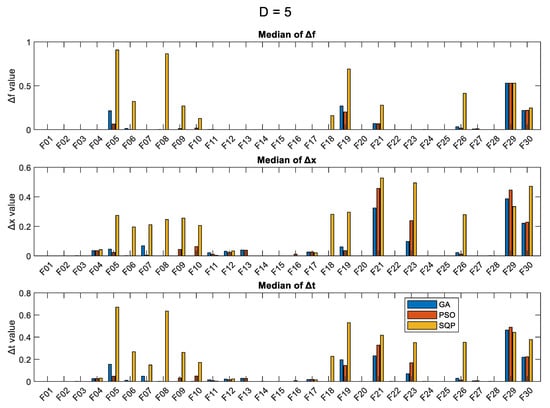
Figure 1.
Results (over 50 runs), for the 3 optimizers, for D = 5, for all 30 objective functions.
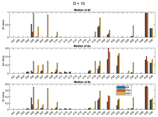
Figure 2.
Results (over 50 runs), for the 3 optimizers, for D = 10, for all 30 objective functions.
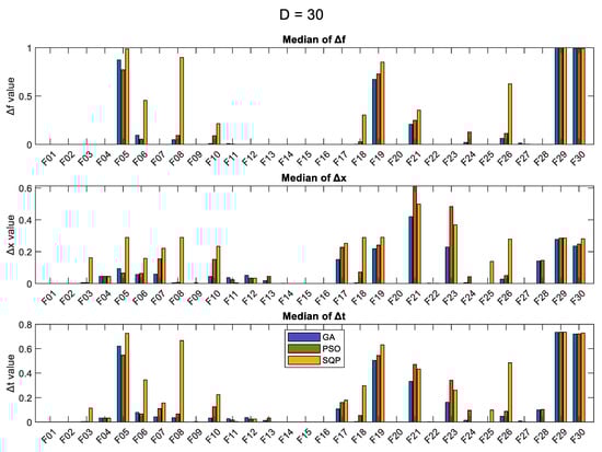
Figure 3.
Results (over 50 runs), for the 3 optimizers, for D = 30, for all 30 objective functions.
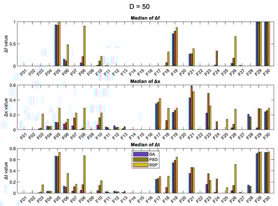
Figure 4.
Results (over 50 runs), for the 3 optimizers, for D = 50, for all 30 objective functions.
More detailed results are presented in table format in Appendix C, where Table A1 shows the results obtained from the three optimizers for the cases D = 5 and D = 10, as averages over 50 runs, and Table A2 shows the corresponding average results for the cases D = 30 and D = 50. Table A3 (cases D = 5 and D = 10) and Table A4 (cases D = 30 and D = 50) show the results obtained from the three optimizers as median values. Table A5 and Table A6 show the standard deviation of the results, for each algorithm and each dimension case. In addition, Table A7 and Table A8 show the median values of the Δx metric, Table A9 and Table A10 show the median values of the Δf metric, and last, Table A11 and Table A12 show the median values of the combined Δt metric.
As expected, the SQP shows the least variance of the results (lowest values of the standard deviation), in most cases, and this is particularly true for higher dimensions. The SQP seems to specialize in some specific problems, such as F01, F02, F13, F14, F15, F16, F20, F24, and F28, where it manages to get very close to the optimum solution, in comparison to the GA and PSO. The values of the Δf and Δx metrics provide a good indication of the performance of the algorithms and which problem is hard to solve. According to the Δf metric, the functions F05, F06, F08, F10, F18, F19, F21, F24, F26, F29, and F30 are hard to optimize, with F29 and F30 being the hardest.
3.2. Convergence History for Each Problem and Each Optimization Algorithm
The convergence histories for each problem and each optimization algorithm for the various numbers of dimensions are presented in the following figures as follows: D = 5 (Figure 5 and Figure 6), D = 10 (Figure 7 and Figure 8), D = 30 (Figure 9 and Figure 10), and D = 50 (Figure 11 and Figure 12), as the median values over 50 runs, for each case. The median is the 0.5 quantile of a data set, i.e., the middle number in a sorted list of numbers. The presentation of these results using the median curve is more descriptive than the one using the average curve, as the median is not affected by the existence of any outliers, in contrast with the average. It should be noted that in these convergence history plots, the y-axis (median of objective function values) is in the logarithmic scale, while the x-axis (number of iterations) remains in the normal scale.
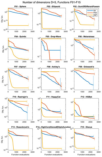
Figure 5.
Convergence histories of the various optimizers for 5 dimensions (D = 5), for the first 15 objective functions, F01 to F15 (median of 50 runs).
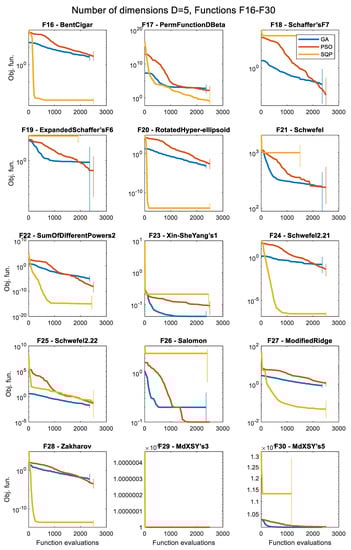
Figure 6.
Convergence histories of the various optimizers for 5 dimensions (D = 5), for the objective functions F16 to F30 (median of 50 runs).
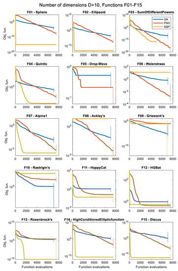
Figure 7.
Convergence histories of the various optimizers for 10 dimensions (D = 10), for the first 15 objective functions, F01 to F15 (median of 50 runs).
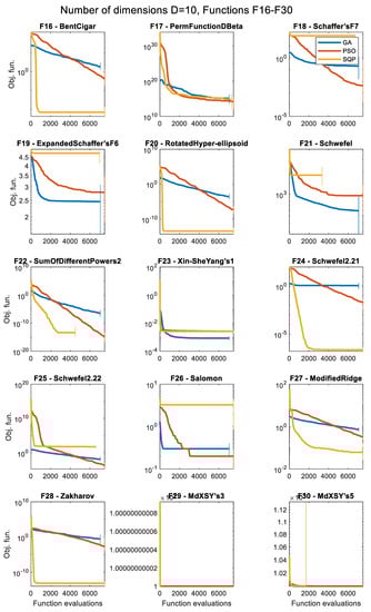
Figure 8.
Convergence histories of the various optimizers for 10 dimensions (D = 10), for the objective functions F16 to F30 (median of 50 runs).
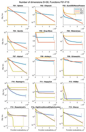
Figure 9.
Convergence histories of the various optimizers for 30 dimensions (D = 30), for the first 15 objective functions, F01 to F15 (median of 50 runs).
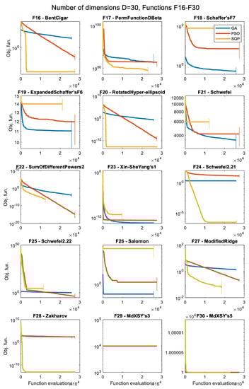
Figure 10.
Convergence histories of the various optimizers for 30 dimensions (D = 30), for the objective functions F16 to F30 (median of 50 runs).
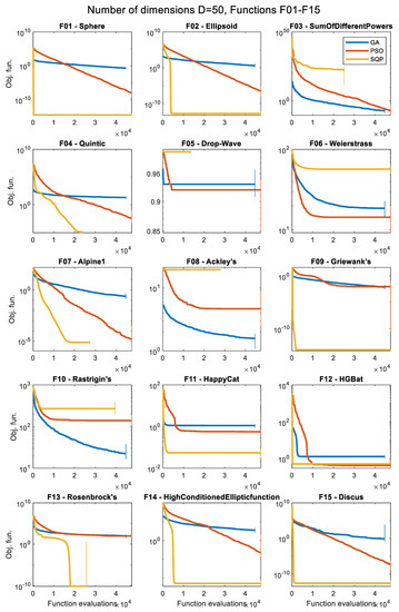
Figure 11.
Convergence histories of the various optimizers for 50 dimensions (D = 50), for the first 15 objective functions, F01 to F15 (median of 50 runs).
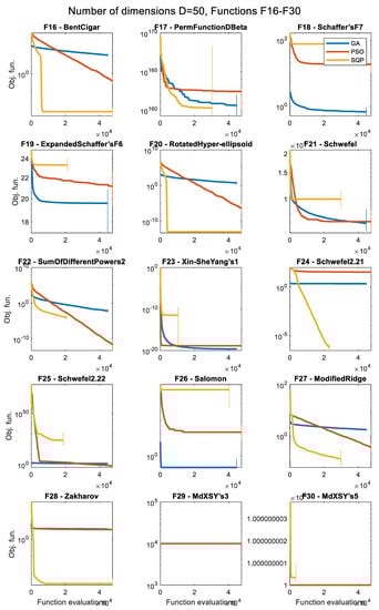
Figure 12.
Convergence histories of the various optimizers for 50 dimensions (D = 50), for the objective functions F16 to F30 (median of 50 runs).
Although the median curve is presented in these figures, there is variation among the 50 independent runs of the algorithms, and it is worth also investigating the spread of these results. For this purpose, at the end of each optimization case (i.e., 50 runs) we calculate the 0.1 quantile, Q0.1 and the 0.9 quantile, Q0.9. The 0.1 quantile is the 10th percentile, i.e., the point where 10% percent of the data have values less than this number. Similarly, the 0.9 quantile is the 90th percentile, i.e., the point where 90% percent of the data have values less than this number. In our case, with 50 elements (50 runs), these two correspond to the average of the 5th and the 6th elements (Q0.1), and the average of the 45th and the 46th elements (Q0.9) of the ordered list containing, in ascending order, the values of the objective function (50 elements in total). Within this range [Q0.1, Q0.9], there are 80% of the values of the objective function (i.e., 40 values in our case).
We see that in some cases this vertical line is long, i.e., there is a large spread of the results above and below the median value, while in other cases the line is barely drawn or it is not drawn at all, i.e., the spread of the results is small. Again, it should be emphasized that this vertical line is drawn along an axis which is presented in a logarithmic scale, and for this reason its top part (the part above the median) would be drawn shorter in length, in comparison to the bottom part (below the median), in a case where the two actually have the same length in absolute values.
4. Discussion and Conclusions
There are plenty of data to be analyzed from the total number of 18,000 optimization problems that are solved. The number of unique problems is in fact 360, since each problem is solved 50 times, to compute the average, the median, and other statistical quantities and evaluation metrics for every algorithm and every problem. The presented results and the convergence histories show both the relevant difficulty of each optimization problem, in the given range of dimensions, and also a comparison of the performance of the different optimization algorithms in each problem.
Every function has its own unique characteristics, and every optimization algorithm has its own special features, advantages, and drawbacks. Some functions are easily optimized by all algorithms, while others pose a real challenge to some (or even all) of the optimizers. It appears to be impossible to establish a single criterion to determine the complexity of the functions; however, we will try to provide a general overview by identifying some common patterns found in the results. In the following, we will use the labels “low”, “middle”, and “high” to estimate the function’s complexity relative to the challenge that they pose to each optimizer.
The convergence history plots shown in Figure 5, Figure 6, Figure 7, Figure 8, Figure 9, Figure 10, Figure 11 and Figure 12 provide an overall picture on how easy or difficult the process of finding the minimum value for an optimization algorithm is, for each problem. If the curve shows a steady decrease towards the zero value early in the process, it means that the algorithm is working as intended for the specific problem, and it is a sign of good performance. When the curve is horizontal at a point above zero, it means that the algorithm is trapped in a local minimum, and it cannot move further. Note that the results presented as convergence history plots are median values over 50 runs, for all three algorithms, the GA, PSO, and SQP. The combined Δt metric can also give us a good indication of the success of each algorithm in each problem.
The first major pattern found is with functions that appear to be easily solvable by the deterministic SQP approach but much more difficult for the GA or the PSO metaheuristics. These functions are, namely: F01, F02, F04, F11, F12, F13, F14, F15, F16, F20, F24, F27, and F28. Such an observation is not a surprise, as these functions are convex and/or unimodal and pure mathematical methods usually excel in such problems, taking advantage of gradient information. Nevertheless, in most of these cases, it appears that increasing the number of iterations may improve the result for the GA or PSO. These functions are classified as a low level of complexity for the SQP and between the low to middle level for the GA and PSO.
The next distinction is made for problems that show a good convergence history curve (i.e., steady decrease towards zero) in all the tested dimensions, but are considered only for the metaheuristics, i.e., the GA or the PSO algorithms. In other words, they are relatively easily solvable by at least one of the tested metaheuristic approaches. The SQP is not considered here to avoid comparing results based on algorithms that serve very different purposes. The identified functions with this characteristic are: F01, F02, F03, F04, F07, F09, F10, F14, F16, F20, F22, F23, F26, and F27. These functions are classified as a low to middle level of complexity for optimizers that are based on metaheuristic approaches.
Functions with a high level of complexity are considered as the ones where none of the algorithms considered seem to have found a satisfactory solution that lays close to the global minimum in at least one of the tested dimensions. Functions with such properties are: F05, F06, F08, F17, F18, F19, F21, F23, F25, F29, and F30. Some of these functions are difficult only in higher dimensions (i.e., D = 30 or D = 50), while others, such as F05, F17, F29, and F30 are very challenging in all the tested dimensions, even for the simplest D = 5 case. Most of these functions are nonconvex and multimodal and the optimizers get trapped in local minima quite often. For the last two functions, F29 and F30, although the optimum point is clearly visible in the 2D case, as shown in Figure A30 and Figure A31, respectively, it is extremely difficult to locate it in practice using optimization procedures. Due to the presence of numerous local minima and the isolation of the global minimum, these two problems represent difficult “needle in a haystack” optimization cases that are extremely hard to optimize effectively. In both problems F29 and F30, all three optimizers fail to reach objective function values lower than 10,000 in all dimension cases, even for the simplest D = 5 case. Based on some additional tests that were performed, it appears that the task is very challenging even when only two dimensions are considered (case D = 2).
The three optimizers, GA, PSO, and SQP, in their MATLAB implementations require different computational times to end up to the optimum solutions. In general, the PSO was found to be the fastest algorithm in all the examined problems. In most cases, the SQP was the slowest algorithm, requiring more time than the GA, especially when low-dimensional spaces were examined (D = 5 or D = 10 cases). The needed time for each algorithm and each problem is recorded by the program and the relevant results are available in the github repository hosting the source code of the project.
5. User Notes
A dedicated github repository, freely available at https://github.com/vplevris/Collection30Functions (accessed on 24 February 2022), has been made for this project, where the interested reader can download the code, run it, and reproduce all the results and the data of the paper, including tables, figures, etc. A detailed instruction file is also provided in Word format on how to run the different modules of the code.
Author Contributions
Conceptualization, V.P.; methodology, V.P.; software, V.P. and G.S.; validation, V.P. and G.S.; formal analysis, V.P. and G.S.; investigation, V.P. and G.S.; resources, V.P. and G.S.; data curation, V.P. and G.S.; writing—original draft preparation, V.P. and G.S.; writing—review and editing, V.P. and G.S.; visualization, V.P. and G.S.; supervision, V.P.; project administration, V.P.; funding acquisition, G.S. All authors have read and agreed to the published version of the manuscript.
Funding
The APC was funded by Oslo Metropolitan University.
Institutional Review Board Statement
Not applicable.
Informed Consent Statement
Not applicable.
Data Availability Statement
The full source code of the study, including the 30 functions, the 3 optimizers, and the full methodology, are provided. The code is written in MATLAB. Any reader can download the source code, run it in MATLAB, and reproduce the results of the study. It is available online at https://github.com/vplevris/Collection30Functions (accessed on 24 February 2022).
Conflicts of Interest
The authors declare no conflict of interest.
Appendix A. Detailed Description of the 30 Functions
The properties, mathematical formulation, suggested search space, and the location of the global minimum are given in detail for each function in this appendix. In addition, the 30 functions are plotted for the simple two-dimensional case (D = 2), to provide a visual idea of their shapes and complexities. For each function, there are two plots. The one on the right (b) provides a general overview as the plotting area is set to the suggested search range according to Table 2. The plot on the left (a) is a closer look (or a zoom-in) into the search area by a factor of ×10 (in other words, the plot range is limited to 1/10 of the suggested search range).
1. Sphere function (sphere_func)
The Sphere function [32], also known as De Jong’s function [33] is one of the simplest optimization test functions, probably the simplest, easiest, and most commonly used continuous domain search problem. It is continuous, convex, unimodal, differentiable, separable, highly symmetric, and rotationally invariant. The suggested search area is the hypercube [−100, 100]D. The global minimum is f01(x*) = 0 at x* = {0, 0, …, 0}. The general formulation of the function is:
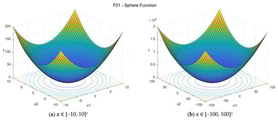
Figure A1.
F01—Sphere function in two dimensions.
2. Ellipsoid function (ellipsoid_func)
The Ellipsoid function [32], or Hyper-ellipsoid function or Axis Parallel Hyper-ellipsoid function, is similar to the sphere function and it is also known as the Weighted sphere function [33]. It is continuous, convex, differentiable, separable, and unimodal. The suggested search area is the hypercube [−100, 100]D. The global minimum is f02(x*) = 0 at x* = {0, 0, …, 0}. The general formulation of the function is:
3. Sum of Different Powers function (sumpow_func)
The Sum of Different Powers function [33] is a commonly used unimodal test function. The suggested search area is the hypercube [−10, 10]D. The global minimum is f03(x*) = 0 at x* = {0, 0, …, 0}. The general formulation of the function is:
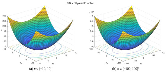
Figure A2.
F02—Ellipsoid function in two dimensions.
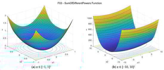
Figure A3.
F03—Sum of Different Powers function in two dimensions.
4. Quintic function (quintic_func)
The Quintic function has the following general formulation:
The suggested search area is the hypercube [−20, 20]D. The function has two distinct global minima with f04(x*) = 0 at x* = {−1, −1, …, −1} or x* = {2, 2, …, 2}.
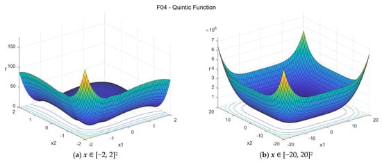
Figure A4.
F04—Quintic function in two dimensions.
5. Drop-Wave function (drop_wave_func)
The Drop-Wave function is a multimodal function with high complexity. The suggested search area is the hypercube [−5.12, 5.12]D. The global minimum is f05(x*) = 0 at x* = {0, 0, …, 0}. The general formulation of the function is:
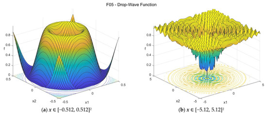
Figure A5.
F05—Drop-Wave function in two dimensions.
6. Weierstrass function (weierstrass_func)
The Weierstrass function [32] is multimodal and it is continuous everywhere but only differentiable on a set of points. It is a computationally expensive function. The suggested search area is the hypercube [−0.5, 0.5]D. In this search area, the global minimum is unique, and it is f06(x*) = 0 at x* = {0, 0, …, 0}. Note that if a larger search area is considered, then there might be multiple global optima as the function is periodic. For this reason, it is strongly suggested to use the previously mentioned search area of [−0.5, 0.5]D. The general formulation of the function is:
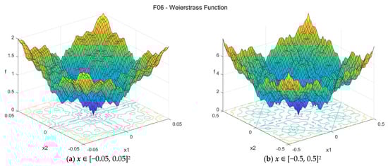
Figure A6.
F06—Weierstrass function in two dimensions.
7. Alpine 1 function (alpine1_func)
The Alpine 1 function is a non-convex multimodal differentiable function. The suggested search area is the hypercube [−10, 10]D. The global minimum is f07(x*) = 0 at x* = {0, 0, …, 0}. The general formulation of the function is:
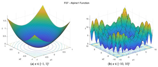
Figure A7.
F07—Alpine 1 function in two dimensions.
8. Ackley’s function (ackley_func)
The Ackley’s function [32,33,34] is non-convex and multimodal, having many local optima with the global optimum located in a very small basin. The suggested search area is the hypercube [−32.768, 32.768]D. The global minimum is f08(x*) = 0 at x* = {0, 0, …, 0}. The general formulation of the function is:
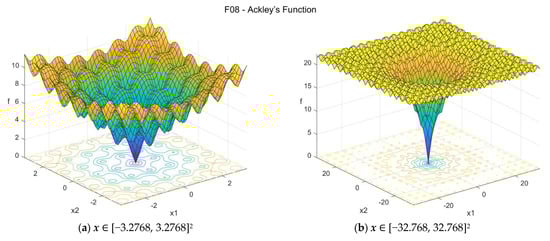
Figure A8.
F08—Ackley’s function in two dimensions.
9. Griewank’s function (griewank_func)
The Griewank’s function [32,33] is a multimodal function which has many regularly distributed local minima. The suggested search area is the hypercube [−100, 100]D. The global minimum is f09(x*) = 0 at x* = {0, 0, …, 0}. The general formulation of the function is:
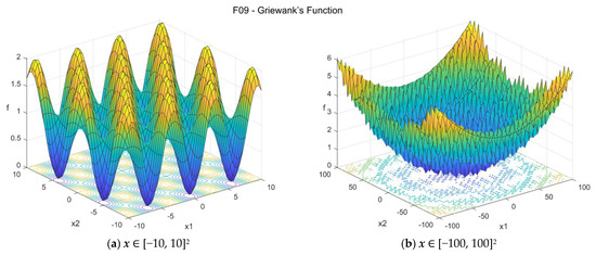
Figure A9.
F09—Griewank’s function in two dimensions.
10. Rastrigin’s function (rastrigin_func)
Rastrigin’s function [32,33,34] is highly multimodal, with many regularly distributed local optima (roughly 10D local optima). The suggested search area is the hypercube [−5.12, 5.12]D. The global minimum is f10(x*) = 0 at x* = {0, 0, …, 0}. The general formulation of the function is:
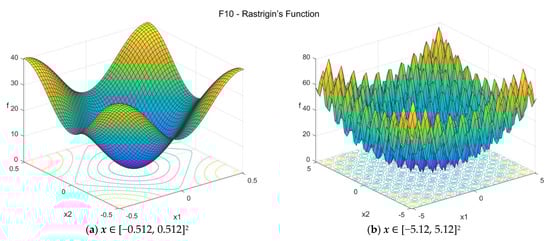
Figure A10.
F10—Rastrigin’s function in two dimensions.
11. HappyCat function (happycat_func)
The HappyCat function [32] is multimodal, with the global minimum located in curved narrow valley. The suggested search area is the hypercube [−20, 20]D. The global minimum is f11(x*) = 0 at x* = {−1, −1, …, −1}. The general formulation of the function is:
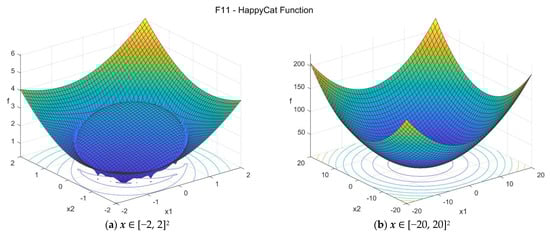
Figure A11.
F11—HappyCat function in two dimensions.
12. HGBat function (hgbat_func)
The HGBat function [32] is similar to HappyCat function but it is even more complex. It is a multimodal function. The suggested search area is the hypercube [−15, 15]D. The global minimum is f12(x*) = 0 at x* = {−1, −1, …, −1}. The general formulation of the function is:
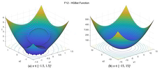
Figure A12.
F12—HGBat function in two dimensions.
13. Rosenbrock’s function (rosenbrock_func)
The Rosenbrock’s function [33] is a classic optimization problem also known as Rosenbrock’s valley or Banana function. The global optimum lays inside a long, narrow, parabolic shaped flat valley. Finding the valley is trivial, but convergence to the global optimum is difficult. The suggested search area is the hypercube [−10, 10]D. The global minimum is f13(x*) = 0 at x* = {1, 1, …, 1}. The general formulation of the function is:
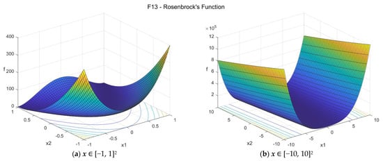
Figure A13.
F13—Rosenbrock’s function in two dimensions.
14. High Conditioned Elliptic function (ellipt_func)
The High Conditioned Elliptic function [32] is a unimodal, globally quadratic, and ill-conditioned function with smooth local irregularities. The suggested search area is the hypercube [−100, 100]D. The global minimum is f14(x*) = 0 at x* = {0, 0, …, 0}. The general formulation of the function is:
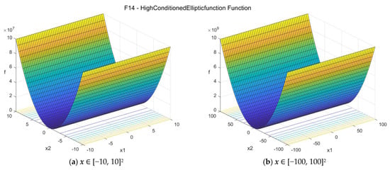
Figure A14.
F14—High Conditioned Elliptic function in two dimensions.
15. Discus function (discus_func)
The Discus function is a globally quadratic unimodal function with smooth local irregularities where a single direction in the search space is thousands of times more sensitive than all others (conditioning is about 106). The suggested search area is the hypercube [−100, 100]D. The global minimum is f15(x*) = 0 at x* = {0, 0, …, 0}. The general formulation of the function is:
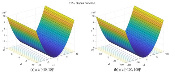
Figure A15.
F15—Discus function in two dimensions.
16. Bent Cigar function (bent_cigar_func)
The Bent Cigar function is unimodal and nonseparable, with the optimum located in a smooth, but very narrow valley. The suggested search area is the hypercube [−100, 100]D. The global minimum is f16(x*) = 0 at x* = {0, 0, …, 0}. The general formulation of the function is:
We notice that in the 2D case, functions f14, f15, and f16 give essentially the same optimization problem, but for D > 2 this is not the case.
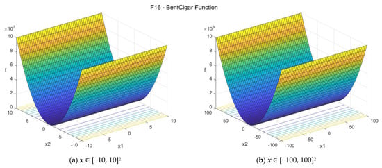
Figure A16.
F16—Bent Cigar function in two dimensions.
17. Perm D, Beta function (permdb_func)
The Perm D, Beta function is a unimodal function. The suggested search area is the hypercube [−D, D]D. This is because the global minimum f17(x*) = 0 is at x* = {1, 2, …, D}, to ensure that it will always lie inside the search area. In the present study, since D = 50 is the max. number of dimensions considered, and to keep things consistent, we will use the search range [−50, 50]D for all the cases considered (for all dimensions).
The general formulation of the function is:
Figure A17 depicts the function in the 2D case (D = 2) for the search range considered [−50, 50]2 and the zoomed case [−5, 5]2. In this case, the formula is:
By setting β = 0.5 in the 2D case, we obtain:
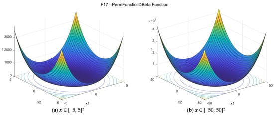
Figure A17.
F17—Perm D, Beta function in two dimensions.
For illustration purposes, Figure A18 depicts the same 2D function in the range [−20, 20]2 and the zoomed case [−2, 2]2.
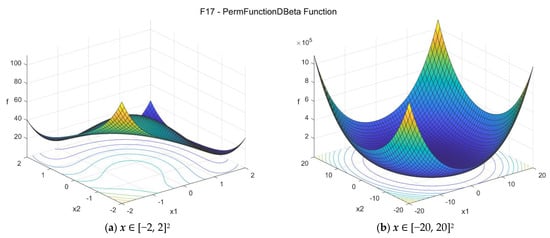
Figure A18.
F17—Perm D, Beta function in two dimensions (closer look).
18. Schaffer’s F7 function (schafferf7_func)
The Schaffer’s F7 function [32,34] is multimodal and nonseparable. The suggested search area is the hypercube [−100, 100]D. The global minimum is f18(x*) = 0 at x* = {0, 0, …, 0}. The general formulation of the function is:
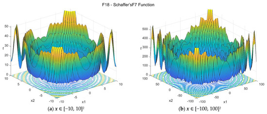
Figure A19.
F18—Schaffer’s F7 function in two dimensions.
19. Expanded Schaffer’s F6 function (expschafferf6_func)
The Expanded Schaffer’s F6 function is a multidimensional function based on the Schaffer’s F6 function [34]. It is multimodal and nonseparable. The suggested search area is the hypercube [−100, 100]D. The global minimum is f19(x*) = 0 at x* = {0, 0, …, 0}. The general formulation of the function is:
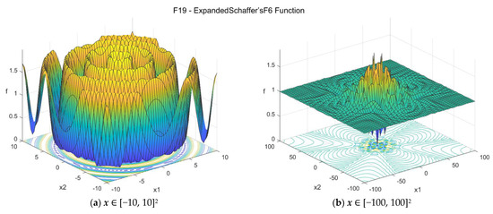
Figure A20.
F19—Expanded Schaffer’s F6 function in two dimensions.
20. Rotated Hyper-ellipsoid function (rothellipsoid_func)
The Rotated Hyper-ellipsoid function is similar to the Ellipsoid function. It is continuous, convex, and unimodal. The suggested search area is the hypercube [−100, 100]D. The global minimum is f20(x*) = 0 at x* = {0, 0, …, 0}. The general formulation of the function is:
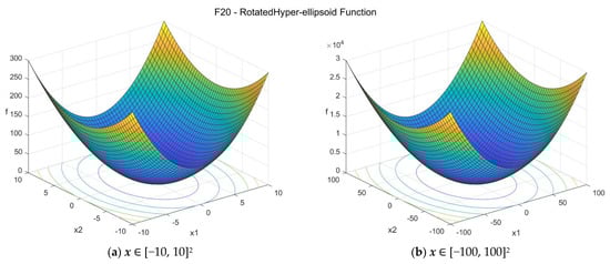
Figure A21.
F20—Rotated Hyper-ellipsoid function in two dimensions.
21. Schwefel function (schwefel_func)
The Schwefel function [33,34] is quite complex, with multiple local minima. The suggested search area is the hypercube [−500, 500]D. The global minimum is f21(x*) = 0 at x* = {c, c, …, c}, where c = 420.968746359982025. The general formulation of the function is:
In the literature, the function is also found with the constant value 418.9829∙D where the optimum location is reported with c = 420.9687 [34]. This formulation is not very precise. For details on this and a relevant detailed investigation of the function, please see Appendix B.
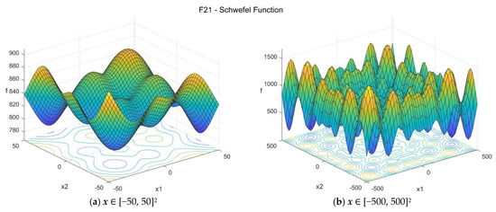
Figure A22.
F21—Schwefel function in two dimensions.
22. Sum of Different Powers 2 function (sumpow2_func)
The Sum of Different Powers 2 function [32] is similar to the Sum of Different Powers function, but its formulation is slightly different. It is unimodal and nonseparable, with different sensitives for the various design variables. The suggested search area is again the hypercube [−10, 10]D. The global minimum is f22(x*) = 0 at x* = {0, 0, …, 0}. The general formulation of the function is:
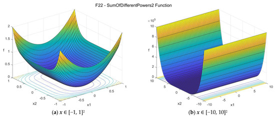
Figure A23.
F22—Sum of Different Powers 2 function in two dimensions.
23. Xin-She Yang’s 1 function (xinsheyang1_func)
The Xin-She Yang’s 1 function [33] is nonconvex and nonseparable. The function is not smooth, and its derivatives are not well-defined at the optimum. The suggested search area is the hypercube [−2π, 2π]D. The global minimum is f23(x*) = 0 at x* = {0, 0, …, 0}. The general formulation of the function is:
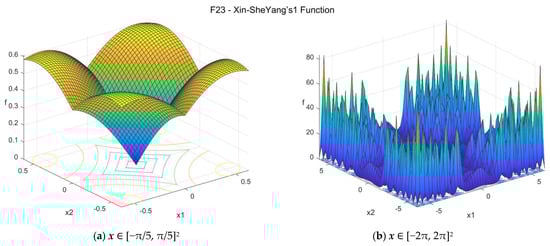
Figure A24.
F23—Xin-She Yang’s 1 function in two dimensions.
24. Schwefel 2.21 function (schwefel221_func)
The Schwefel 2.21 function is convex, continuous, and unimodal. The suggested search area is the hypercube [−100, 100]D. The global minimum is f24(x*) = 0 at x* = {0, 0, …, 0}. The general formulation of the function is:
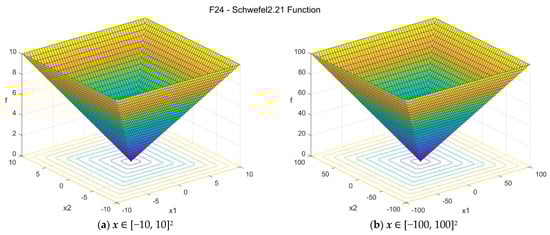
Figure A25.
F24—Schwefel 2.21 function in two dimensions.
25. Schwefel 2.22 function (schwefel222_func)
The Schwefel 2.22 function is convex, continuous, separable, and unimodal. The suggested search area is the hypercube [−100, 100]D. The global minimum is f25(x*) = 0 at x* = {0, 0, …, 0}. The general formulation of the function is:
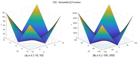
Figure A26.
F25—Schwefel 2.22 function in two dimensions.
26. Salomon function (salomon_func)
The Salomon function is nonconvex, continuous, multimodal, and nonseparable. The suggested search area is the hypercube [−20, 20]D. The global minimum is f26(x*) = 0 at x* = {0, 0, …, 0}. The general formulation of the function is:
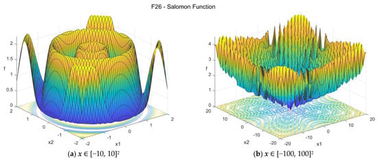
Figure A27.
F26—Salomon function in two dimensions.
27. Modified Ridge function (modridge_func)
The original Ridge function has the form
In this formula, d and a are constants and are usually set to d = 1, a = 0.1. Other values (d = 2, a = 0.5, etc) can be also found in the literature. The Modified Ridge function proposed in this study has the form:
The suggested search area is the hypercube [−100, 100]D. The global minimum is f27(x*) = 0 at x* = {0, 0, …, 0}.
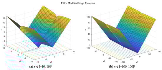
Figure A28.
F27—Ridge function in two dimensions.
28. Zakharov function (zakharov_func)
The Zakharov function is continuous and unimodal. The suggested search area is the hypercube [−10, 10]D. The global minimum is f28(x*) = 0 at x* = {0, 0, …, 0}. The general formulation of the function is:
The suggested search area is the hypercube [−10, 10]D. The global minimum is f28(x*) = 0 at x* = {0, 0, …, 0}.
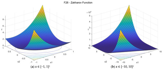
Figure A29.
F28—Zakharov function in two dimensions.
29. Modified Xin-She Yang’s 3 function (modxinsyang3_func)
The original Xin-She Yang’s 3 function is the third function proposed in the excellent work by Xin-She Yang [33]. The Modified Xin-She Yang’s 3 function proposed in this study is based on that, with some modifications. It is a standing-wave function with a defect, which is nonconvex and nonseparable, with multiple local minima, and a unique global minimum. The suggested search area is the hypercube [−20, 20]D. The global minimum is f29(x*) = 0 at x* = {0, 0, …, 0}. The general formulation of the function is:
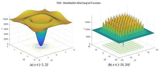
Figure A30.
F29—Modified Xin-She Yang’s 3 function in two dimensions.
30. Modified Xin-She Yang’s 5 function (modxinsyang5_func)
The original Xin-She Yang’s 5 function is the fifth function proposed in the work by Xin-She Yang [33]. The Modified Xin-She Yang’s 5 function proposed in this study is based on that, with some minor modifications. The suggested search area is the hypercube [−100, 100]D. The global minimum is f30(x*) = 0 at x* = {0, 0, …, 0}. The general formulation of the function is:
The function has multiple local minima, but the global minimum is unique. Figure A31 depicts the function in the 2D case (D = 2) where its landscape looks like a wonderful candlestick [33]. The function is simplified as:
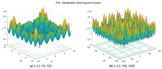
Figure A31.
F30—Modified Xin-She Yang’s 5 function in two dimensions.
Appendix B. Investigation of the Schwefel Function (F21)
In the literature [33,34], the Schwefel function (F21 in this study) is usually found with the value 418.9829∙D in its formula and the optimum location is reported with c = 420.9687. This formulation is not very precise, compared to the formulation described here in the description of the function. Indeed, to find the correct values, one can take the one-dimensional case (D = 1) and find the minimum of the function
in the search area [−500, 500]. A plot of the function of Equation (A63) is presented in Figure A32.
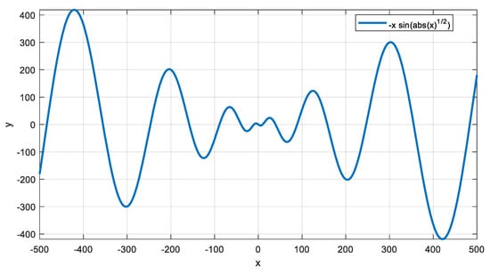
Figure A32.
Plot of the function for −500 < x < 500.
As shown in the figure, the minimum is obviously within the range [400, 500] for x. To find the exact location of the minimum, we can omit the absolute term (since x > 0 in this range) and find the value of x ∈ [400, 500] that makes the derivative of the function equal to zero. In this case, we have:
By using MATLAB and the function “vpasolve”, we can numerically find the root of y’(x) for x ∈ [400, 500] as follows (code in MATLAB):
        syms x y
        y = -x*sin(sqrt(x));
        yd = diff(y,x);
        s = vpasolve(yd = = 0, x, [400 500])
Then we obtain the result:
s = 420.96874635998202731184436501869
We substitute the above s value in the function (as x), to find the minimum value of f, as follows:
fmin = subs(f,x,s)
and we obtain
fmin(x) = −418.9828872724337062747864351956
Practically, there is no need to take into account so many decimal places. In the formulation proposed in this study, the formula for f20 is the following
For the above function, the global minimum is f21(x*) = 0 at x* = {c, c, …, c}, where c = 420.968746359982025.
Appendix C. Tables with the Numerical Results
Table A1.
Average values (over 50 runs) of the optimum results, for the 3 optimizers, for dimensions D = 5 and D = 10.
Table A1.
Average values (over 50 runs) of the optimum results, for the 3 optimizers, for dimensions D = 5 and D = 10.
| ID | Function Name | D = 5 | D = 10 | ||||
|---|---|---|---|---|---|---|---|
| GA | PSO | SQP | GA | PSO | SQP | ||
| F01 | Sphere | 7.59E-04 | 7.37E-03 | 1.38E-14 | 2.52E-04 | 5.65E-08 | 1.05E-15 |
| F02 | Ellipsoid | 1.02E-03 | 2.86E-02 | 9.16E-14 | 1.00E-03 | 2.49E-07 | 1.44E-13 |
| F03 | Sum of Different Powers | 4.25E-05 | 2.70E-07 | 5.68E-11 | 1.85E-06 | 1.52E-14 | 2.64E-08 |
| F04 | Quintic | 2.12E-01 | 2.42E-01 | 3.78E-06 | 1.43E-01 | 2.47E-03 | 2.27E-06 |
| F05 | Drop-Wave | 1.86E-01 | 6.38E-02 | 8.61E-01 | 4.61E-01 | 1.45E-01 | 9.18E-01 |
| F06 | Weierstrass | 3.21E-01 | 4.78E-02 | 5.89E+00 | 7.41E-01 | 1.13E-01 | 1.20E+01 |
| F07 | Alpine 1 | 8.21E-03 | 2.32E-02 | 2.52E-06 | 1.67E-03 | 8.92E-04 | 1.58E-06 |
| F08 | Ackley’s | 2.60E-01 | 3.21E-02 | 1.89E+01 | 1.48E-01 | 4.63E-02 | 1.95E+01 |
| F09 | Griewank’s | 1.48E-02 | 1.58E-01 | 3.35E+00 | 1.10E-02 | 1.46E-01 | 6.38E-01 |
| F10 | Rastrigin’s | 5.93E-01 | 3.49E+00 | 2.55E+01 | 1.10E+00 | 1.10E+01 | 6.77E+01 |
| F11 | HappyCat | 4.66E-01 | 1.89E-01 | 4.18E-02 | 9.48E-01 | 2.39E-01 | 1.56E-01 |
| F12 | HGBat | 5.27E-01 | 2.65E-01 | 4.90E-01 | 8.87E-01 | 4.04E-01 | 5.20E-01 |
| F13 | Rosenbrock’s | 2.57E+00 | 2.54E+00 | 5.50E-01 | 6.50E+00 | 1.35E+01 | 4.78E-01 |
| F14 | High Cond. Elliptic | 7.39E+01 | 6.00E+01 | 3.50E-11 | 4.88E+01 | 5.44E+03 | 3.57E-11 |
| F15 | Discus | 5.80E+02 | 1.86E+02 | 1.50E-11 | 1.92E+03 | 7.16E-06 | 7.18E-12 |
| F16 | Bent Cigar | 7.71E+02 | 2.42E+03 | 1.16E-10 | 9.10E+01 | 3.15E+01 | 9.83E-11 |
| F17 | Perm D, Beta | 3.86E+03 | 7.69E+02 | 7.81E+01 | 4.77E+15 | 9.91E+14 | 8.35E+15 |
| F18 | Schaffer’s F7 | 3.08E-01 | 1.01E-01 | 7.12E+01 | 3.76E-01 | 1.50E-01 | 7.24E+01 |
| F19 | Expanded Schaffer’s F6 | 9.11E-01 | 7.40E-01 | 2.32E+00 | 2.40E+00 | 2.76E+00 | 4.64E+00 |
| F20 | Rotated Hyper-ellipsoid | 2.03E-03 | 9.91E-03 | 6.24E-14 | 6.20E-04 | 1.30E-07 | 8.83E-14 |
| F21 | Schwefel | 2.58E+02 | 2.84E+02 | 9.63E+02 | 5.80E+02 | 9.50E+02 | 1.83E+03 |
| F22 | Sum of Dif. Powers 2 | 5.61E-05 | 8.71E-07 | 9.31E-13 | 1.54E-06 | 7.59E-14 | 1.91E-10 |
| F23 | Xin-She Yang’s 1 | 4.84E-02 | 9.07E-02 | 1.68E-01 | 8.94E-04 | 2.60E-03 | 2.56E-03 |
| F24 | Schwefel 2.21 | 4.13E-01 | 6.92E-02 | 2.81E-07 | 1.26E+00 | 2.60E-02 | 2.59E-07 |
| F25 | Schwefel 2.22 | 2.24E-02 | 2.51E-01 | 5.09E+00 | 5.87E-02 | 4.81E-04 | 6.53E+01 |
| F26 | Salomon | 2.50E-01 | 1.06E-01 | 2.16E+00 | 3.08E-01 | 2.10E-01 | 3.11E+00 |
| F27 | Modified Ridge | 8.25E-01 | 1.09E+00 | 6.08E-02 | 7.40E-01 | 3.32E-01 | 8.00E-02 |
| F28 | Zakharov | 2.50E-01 | 2.54E-03 | 6.01E-14 | 1.95E+00 | 2.03E+00 | 8.05E-14 |
| F29 | Mod. Xin-She Yang’s 3 | 1.00E+04 | 1.00E+04 | 1.00E+04 | 1.00E+04 | 1.00E+04 | 1.00E+04 |
| F30 | Mod. Xin-She Yang’s 5 | 9.61E+03 | 1.00E+04 | 1.15E+04 | 1.00E+04 | 1.00E+04 | 1.03E+04 |
Table A2.
Average values (over 50 runs) of the optimum results, for the 3 optimizers, for dimensions D = 30 and D = 50.
Table A2.
Average values (over 50 runs) of the optimum results, for the 3 optimizers, for dimensions D = 30 and D = 50.
| ID | Function Name | D = 30 | D = 50 | ||||
|---|---|---|---|---|---|---|---|
| GA | PSO | SQP | GA | PSO | SQP | ||
| F01 | Sphere | 1.77E-02 | 3.43E-10 | 3.38E-15 | 2.34E-01 | 3.46E-06 | 6.00E-15 |
| F02 | Ellipsoid | 2.63E-01 | 9.61E-09 | 3.26E-13 | 5.35E+00 | 1.12E-04 | 2.87E-13 |
| F03 | Sum of Different Powers | 1.30E-07 | 2.33E-11 | 1.93E+10 | 6.21E-06 | 1.98E+00 | 3.64E+25 |
| F04 | Quintic | 5.76E+00 | 3.20E-03 | 6.61E-06 | 2.06E+01 | 1.89E-01 | 1.76E-05 |
| F05 | Drop-Wave | 8.67E-01 | 7.27E-01 | 9.85E-01 | 9.30E-01 | 9.10E-01 | 9.72E-01 |
| F06 | Weierstrass | 7.89E+00 | 4.47E+00 | 3.60E+01 | 1.88E+01 | 1.45E+01 | 5.70E+01 |
| F07 | Alpine 1 | 3.81E-02 | 2.05E-06 | 4.47E-06 | 2.59E-01 | 2.72E-04 | 7.77E-06 |
| F08 | Ackley’s | 9.51E-01 | 2.02E+00 | 1.95E+01 | 1.52E+00 | 5.37E+00 | 1.95E+01 |
| F09 | Griewank’s | 4.43E-03 | 1.50E-02 | 1.48E-14 | 9.88E-03 | 3.86E-02 | 1.06E-14 |
| F10 | Rastrigin’s | 8.32E+00 | 8.37E+01 | 1.78E+02 | 2.44E+01 | 1.51E+02 | 2.84E+02 |
| F11 | HappyCat | 1.07E+00 | 4.86E-01 | 7.18E-02 | 1.12E+00 | 5.81E-01 | 6.50E-02 |
| F12 | HGBat | 1.18E+00 | 6.06E-01 | 5.00E-01 | 1.25E+00 | 5.86E-01 | 5.00E-01 |
| F13 | Rosenbrock’s | 3.88E+01 | 5.27E+01 | 1.36E+00 | 9.74E+01 | 9.53E+01 | 7.97E-01 |
| F14 | High Cond. Elliptic | 1.72E+02 | 5.10E+01 | 1.46E-11 | 1.05E+03 | 5.90E+02 | 7.28E-12 |
| F15 | Discus | 1.03E+03 | 2.00E+02 | 5.12E-12 | 2.24E+03 | 3.03E-07 | 6.01E-13 |
| F16 | Bent Cigar | 1.26E+04 | 1.10E-03 | 1.62E-10 | 2.08E+05 | 3.48E-01 | 5.71E-10 |
| F17 | Perm D, Beta | 7.45E+86 | 7.19E+82 | 1.10E+80 | 8.96E+161 | 6.44E+162 | 2.34E+168 |
| F18 | Schaffer’s F7 | 5.36E-01 | 7.84E+00 | 7.59E+01 | 6.83E-01 | 1.80E+01 | 7.56E+01 |
| F19 | Expanded Schaffer’s F6 | 1.08E+01 | 1.17E+01 | 1.39E+01 | 1.94E+01 | 2.10E+01 | 2.33E+01 |
| F20 | Rotated Hyper-ellipsoid | 3.74E-01 | 4.43E-09 | 2.14E-13 | 6.73E+00 | 2.53E-05 | 3.00E-13 |
| F21 | Schwefel | 3.42E+03 | 4.07E+03 | 5.77E+03 | 7.10E+03 | 7.20E+03 | 9.96E+03 |
| F22 | Sum of Dif. Powers 2 | 3.01E-04 | 1.70E-14 | 1.05E-06 | 1.33E-02 | 7.21E-11 | 1.01E-04 |
| F23 | Xin-She Yang’s 1 | 7.13E-12 | 2.56E-11 | 7.03E-10 | 2.47E-20 | 1.35E-19 | 1.02E-10 |
| F24 | Schwefel 2.21 | 2.03E+00 | 1.34E+01 | 4.81E-07 | 2.17E+00 | 3.34E+01 | 8.34E-07 |
| F25 | Schwefel 2.22 | 1.10E+00 | 2.20E+00 | 1.12E+08 | 5.80E+00 | 7.00E+00 | 5.61E+55 |
| F26 | Salomon | 5.78E-01 | 1.05E+00 | 5.85E+00 | 7.54E-01 | 2.11E+00 | 7.31E+00 |
| F27 | Modified Ridge | 1.34E+00 | 2.18E-01 | 8.87E-02 | 1.73E+00 | 4.57E-01 | 1.59E-01 |
| F28 | Zakharov | 2.48E+02 | 2.41E+02 | 1.35E-13 | 8.32E+02 | 6.12E+02 | 1.40E-12 |
| F29 | Mod. Xin-She Yang’s 3 | 1.00E+04 | 1.00E+04 | 1.00E+04 | 1.00E+04 | 1.00E+04 | 1.00E+04 |
| F30 | Mod. Xin-She Yang’s 5 | 1.00E+04 | 1.00E+04 | 1.00E+04 | 1.00E+04 | 1.00E+04 | 1.00E+04 |
Table A3.
Median values (over 50 runs) of the optimum results, for the 3 optimizers, for dimensions D = 5 and D = 10.
Table A3.
Median values (over 50 runs) of the optimum results, for the 3 optimizers, for dimensions D = 5 and D = 10.
| ID | Function Name | D = 5 | D = 10 | ||||
|---|---|---|---|---|---|---|---|
| GA | PSO | SQP | GA | PSO | SQP | ||
| F01 | Sphere | 3.48E-04 | 6.70E-04 | 3.77E-16 | 7.29E-05 | 1.95E-08 | 6.72E-16 |
| F02 | Ellipsoid | 4.27E-04 | 3.72E-03 | 1.59E-14 | 2.46E-04 | 2.40E-08 | 4.64E-14 |
| F03 | Sum of Different Powers | 1.23E-05 | 7.91E-09 | 1.71E-15 | 1.59E-07 | 1.72E-17 | 1.78E-12 |
| F04 | Quintic | 1.56E-01 | 1.27E-01 | 1.02E-06 | 7.70E-02 | 3.41E-04 | 2.02E-06 |
| F05 | Drop-Wave | 2.14E-01 | 6.38E-02 | 9.08E-01 | 5.22E-01 | 2.14E-01 | 9.57E-01 |
| F06 | Weierstrass | 2.59E-01 | 3.78E-02 | 5.68E+00 | 6.27E-01 | 1.48E-03 | 1.19E+01 |
| F07 | Alpine 1 | 2.89E-03 | 8.94E-04 | 7.31E-07 | 8.03E-04 | 5.09E-06 | 1.35E-06 |
| F08 | Ackley’s | 2.80E-02 | 1.35E-02 | 1.92E+01 | 1.04E-02 | 4.93E-05 | 1.96E+01 |
| F09 | Griewank’s | 9.05E-05 | 1.41E-01 | 3.29E+00 | 6.29E-06 | 8.27E-02 | 6.52E-02 |
| F10 | Rastrigin’s | 6.30E-02 | 2.93E+00 | 2.24E+01 | 9.95E-01 | 8.95E+00 | 6.57E+01 |
| F11 | HappyCat | 3.67E-01 | 1.73E-01 | 3.72E-02 | 1.00E+00 | 2.42E-01 | 1.29E-01 |
| F12 | HGBat | 4.29E-01 | 2.43E-01 | 4.99E-01 | 8.92E-01 | 3.88E-01 | 5.00E-01 |
| F13 | Rosenbrock’s | 2.07E+00 | 1.88E+00 | 5.29E-11 | 4.05E+00 | 6.03E+00 | 6.02E-11 |
| F14 | High Cond. Elliptic | 1.58E+01 | 1.46E+00 | 4.69E-11 | 1.69E+00 | 3.23E-04 | 2.03E-11 |
| F15 | Discus | 6.04E+00 | 4.27E-02 | 1.18E-12 | 5.51E-01 | 1.81E-07 | 3.50E-13 |
| F16 | Bent Cigar | 2.31E+02 | 2.78E+02 | 5.35E-11 | 1.84E+01 | 1.14E-02 | 1.61E-11 |
| F17 | Perm D, Beta | 7.01E+02 | 1.60E+02 | 1.13E-01 | 1.37E+15 | 1.60E+14 | 5.98E+14 |
| F18 | Schaffer’s F7 | 1.12E-01 | 2.62E-02 | 7.55E+01 | 1.92E-01 | 4.29E-03 | 7.61E+01 |
| F19 | Expanded Schaffer’s F6 | 9.48E-01 | 7.07E-01 | 2.43E+00 | 2.46E+00 | 2.78E+00 | 4.73E+00 |
| F20 | Rotated Hyper-ellipsoid | 7.04E-04 | 2.34E-03 | 1.18E-14 | 2.37E-04 | 4.37E-08 | 3.27E-14 |
| F21 | Schwefel | 2.47E+02 | 2.38E+02 | 9.98E+02 | 5.83E+02 | 9.51E+02 | 1.83E+03 |
| F22 | Sum of Dif. Powers 2 | 9.14E-06 | 8.51E-09 | 9.93E-16 | 2.93E-07 | 2.00E-15 | 4.16E-14 |
| F23 | Xin-She Yang’s 1 | 4.18E-02 | 9.14E-02 | 2.09E-01 | 8.53E-04 | 2.62E-03 | 2.62E-03 |
| F24 | Schwefel 2.21 | 1.56E-01 | 4.51E-02 | 2.77E-07 | 1.13E+00 | 1.74E-02 | 2.32E-07 |
| F25 | Schwefel 2.22 | 1.93E-02 | 4.86E-02 | 1.09E-01 | 1.24E-02 | 1.88E-04 | 5.64E+01 |
| F26 | Salomon | 2.00E-01 | 9.99E-02 | 2.50E+00 | 3.00E-01 | 2.00E-01 | 3.25E+00 |
| F27 | Modified Ridge | 8.25E-01 | 1.08E+00 | 4.80E-02 | 7.30E-01 | 3.17E-01 | 6.13E-02 |
| F28 | Zakharov | 5.72E-03 | 3.89E-04 | 4.06E-14 | 2.44E-01 | 1.84E-03 | 6.49E-14 |
| F29 | Mod. Xin-She Yang’s 3 | 1.00E+04 | 1.00E+04 | 1.00E+04 | 1.00E+04 | 1.00E+04 | 1.00E+04 |
| F30 | Mod. Xin-She Yang’s 5 | 1.00E+04 | 1.00E+04 | 1.13E+04 | 1.00E+04 | 1.00E+04 | 1.00E+04 |
Table A4.
Median values (over 50 runs) of the optimum results, for the 3 optimizers, for dimensions D = 30 and D = 50.
Table A4.
Median values (over 50 runs) of the optimum results, for the 3 optimizers, for dimensions D = 30 and D = 50.
| ID | Function Name | D = 30 | D = 50 | ||||
|---|---|---|---|---|---|---|---|
| GA | PSO | SQP | GA | PSO | SQP | ||
| F01 | Sphere | 1.41E-02 | 5.30E-11 | 2.84E-15 | 1.84E-01 | 7.70E-09 | 2.55E-15 |
| F02 | Ellipsoid | 1.64E-01 | 6.66E-10 | 7.86E-14 | 3.75E+00 | 2.69E-07 | 1.48E-13 |
| F03 | Sum of Different Powers | 1.63E-08 | 1.84E-17 | 4.73E+07 | 7.15E-08 | 9.87E-08 | 1.44E+22 |
| F04 | Quintic | 3.77E+00 | 1.09E-04 | 6.30E-06 | 2.05E+01 | 3.78E-03 | 1.14E-05 |
| F05 | Drop-Wave | 8.73E-01 | 7.70E-01 | 9.85E-01 | 9.31E-01 | 9.20E-01 | 9.91E-01 |
| F06 | Weierstrass | 7.52E+00 | 4.24E+00 | 3.62E+01 | 1.86E+01 | 1.43E+01 | 5.71E+01 |
| F07 | Alpine 1 | 2.34E-02 | 3.99E-07 | 4.41E-06 | 2.30E-01 | 1.53E-05 | 7.75E-06 |
| F08 | Ackley’s | 1.06E+00 | 2.01E+00 | 1.96E+01 | 1.58E+00 | 4.67E+00 | 1.96E+01 |
| F09 | Griewank’s | 7.26E-04 | 9.86E-03 | 1.49E-14 | 7.64E-03 | 9.86E-03 | 1.05E-14 |
| F10 | Rastrigin’s | 6.73E+00 | 7.21E+01 | 1.73E+02 | 2.25E+01 | 1.38E+02 | 2.70E+02 |
| F11 | HappyCat | 1.06E+00 | 4.46E-01 | 5.49E-02 | 1.12E+00 | 5.69E-01 | 5.54E-02 |
| F12 | HGBat | 1.18E+00 | 5.24E-01 | 5.00E-01 | 1.27E+00 | 4.10E-01 | 5.00E-01 |
| F13 | Rosenbrock’s | 1.52E+01 | 2.94E+01 | 6.33E-11 | 9.95E+01 | 9.42E+01 | 6.59E-11 |
| F14 | High Cond. Elliptic | 3.79E+01 | 3.47E-06 | 5.14E-12 | 5.98E+02 | 6.28E-04 | 3.86E-12 |
| F15 | Discus | 1.25E-01 | 7.42E-10 | 4.47E-13 | 7.54E-01 | 5.49E-08 | 2.65E-13 |
| F16 | Bent Cigar | 8.42E+03 | 8.94E-05 | 4.46E-11 | 1.50E+05 | 1.20E-02 | 5.15E-11 |
| F17 | Perm D, Beta | 6.98E+82 | 6.14E+82 | 7.92E+78 | 3.62E+160 | 2.62E+162 | 1.88E+160 |
| F18 | Schaffer’s F7 | 4.97E-01 | 6.93E+00 | 7.67E+01 | 6.67E-01 | 1.83E+01 | 7.56E+01 |
| F19 | Expanded Schaffer’s F6 | 1.10E+01 | 1.20E+01 | 1.40E+01 | 1.96E+01 | 2.11E+01 | 2.33E+01 |
| F20 | Rotated Hyper-ellipsoid | 1.89E-01 | 8.18E-10 | 1.49E-13 | 5.87E+00 | 4.16E-07 | 1.19E-13 |
| F21 | Schwefel | 3.48E+03 | 4.16E+03 | 5.93E+03 | 6.91E+03 | 7.10E+03 | 9.99E+03 |
| F22 | Sum of Dif. Powers 2 | 1.28E-04 | 1.68E-15 | 4.37E-07 | 5.83E-03 | 1.98E-12 | 7.28E-05 |
| F23 | Xin-She Yang’s 1 | 6.75E-12 | 2.53E-11 | 4.41E-10 | 2.35E-20 | 1.36E-19 | 3.38E-12 |
| F24 | Schwefel 2.21 | 2.00E+00 | 1.28E+01 | 2.86E-07 | 2.19E+00 | 3.38E+01 | 6.43E-07 |
| F25 | Schwefel 2.22 | 9.57E-01 | 1.54E-04 | 3.49E+04 | 5.71E+00 | 2.96E-02 | 4.97E+23 |
| F26 | Salomon | 6.00E-01 | 1.10E+00 | 6.10E+00 | 7.00E-01 | 2.10E+00 | 7.85E+00 |
| F27 | Modified Ridge | 1.33E+00 | 2.06E-01 | 6.10E-02 | 1.72E+00 | 3.51E-01 | 1.23E-01 |
| F28 | Zakharov | 2.38E+02 | 2.52E+02 | 8.77E-14 | 8.52E+02 | 5.98E+02 | 1.70E-13 |
| F29 | Mod. Xin-She Yang’s 3 | 1.00E+04 | 1.00E+04 | 1.00E+04 | 1.00E+04 | 1.00E+04 | 1.00E+04 |
| F30 | Mod. Xin-She Yang’s 5 | 1.00E+04 | 1.00E+04 | 1.00E+04 | 1.00E+04 | 1.00E+04 | 1.00E+04 |
Table A5.
Standard deviation (over 50 runs) of the optimum results, for the 3 optimizers, for dimensions D = 5 and D = 10.
Table A5.
Standard deviation (over 50 runs) of the optimum results, for the 3 optimizers, for dimensions D = 5 and D = 10.
| ID | Function Name | D = 5 | D = 10 | ||||
|---|---|---|---|---|---|---|---|
| GA | PSO | SQP | GA | PSO | SQP | ||
| F01 | Sphere | 1.10E-03 | 1.94E-02 | 4.00E-14 | 5.12E-04 | 1.29E-07 | 2.15E-15 |
| F02 | Ellipsoid | 1.43E-03 | 9.20E-02 | 1.65E-13 | 2.56E-03 | 5.30E-07 | 1.88E-13 |
| F03 | Sum of Different Powers | 6.83E-05 | 1.01E-06 | 2.80E-10 | 5.03E-06 | 7.80E-14 | 1.22E-07 |
| F04 | Quintic | 1.46E-01 | 2.93E-01 | 1.48E-05 | 2.28E-01 | 7.64E-03 | 1.20E-06 |
| F05 | Drop-Wave | 1.17E-01 | 7.59E-07 | 1.57E-01 | 1.40E-01 | 8.17E-02 | 1.61E-01 |
| F06 | Weierstrass | 2.32E-01 | 4.01E-02 | 1.22E+00 | 6.43E-01 | 3.62E-01 | 2.38E+00 |
| F07 | Alpine 1 | 1.33E-02 | 8.67E-02 | 7.94E-06 | 2.23E-03 | 5.87E-03 | 1.30E-06 |
| F08 | Ackley’s | 7.18E-01 | 4.49E-02 | 1.64E+00 | 3.72E-01 | 2.26E-01 | 3.44E-01 |
| F09 | Griewank’s | 3.78E-02 | 8.99E-02 | 1.93E+00 | 3.79E-02 | 1.61E-01 | 1.50E+00 |
| F10 | Rastrigin’s | 9.86E-01 | 2.70E+00 | 1.79E+01 | 1.42E+00 | 7.93E+00 | 2.41E+01 |
| F11 | HappyCat | 3.15E-01 | 7.90E-02 | 1.97E-02 | 3.53E-01 | 8.77E-02 | 1.03E-01 |
| F12 | HGBat | 3.42E-01 | 1.06E-01 | 8.07E-02 | 3.39E-01 | 1.38E-01 | 1.45E-01 |
| F13 | Rosenbrock’s | 4.00E+00 | 2.23E+00 | 1.36E+00 | 1.26E+01 | 2.65E+01 | 1.30E+00 |
| F14 | High Cond. Elliptic | 1.49E+02 | 2.08E+02 | 2.89E-11 | 2.56E+02 | 3.07E+04 | 3.68E-11 |
| F15 | Discus | 2.31E+03 | 1.30E+03 | 2.39E-11 | 6.68E+03 | 3.32E-05 | 1.72E-11 |
| F16 | Bent Cigar | 1.65E+03 | 3.71E+03 | 1.35E-10 | 1.95E+02 | 1.93E+02 | 1.69E-10 |
| F17 | Perm D, Beta | 9.50E+03 | 1.47E+03 | 2.54E+02 | 6.62E+15 | 2.43E+15 | 3.01E+16 |
| F18 | Schaffer’s F7 | 4.03E-01 | 2.21E-01 | 2.19E+01 | 4.61E-01 | 3.38E-01 | 1.43E+01 |
| F19 | Expanded Schaffer’s F6 | 5.12E-01 | 3.73E-01 | 2.65E-01 | 5.87E-01 | 5.36E-01 | 2.83E-01 |
| F20 | Rotated Hyper-ellipsoid | 4.67E-03 | 1.82E-02 | 1.05E-13 | 1.04E-03 | 2.66E-07 | 1.24E-13 |
| F21 | Schwefel | 1.49E+02 | 1.62E+02 | 2.92E+02 | 2.40E+02 | 3.07E+02 | 4.08E+02 |
| F22 | Sum of Dif. Powers 2 | 1.30E-04 | 4.42E-06 | 3.74E-12 | 3.07E-06 | 3.22E-13 | 8.59E-10 |
| F23 | Xin-She Yang’s 1 | 1.24E-02 | 2.85E-02 | 5.73E-02 | 2.39E-04 | 1.65E-04 | 7.09E-04 |
| F24 | Schwefel 2.21 | 4.96E-01 | 6.56E-02 | 1.42E-07 | 6.22E-01 | 2.90E-02 | 1.05E-07 |
| F25 | Schwefel 2.22 | 1.50E-02 | 1.23E+00 | 1.37E+01 | 1.75E-01 | 1.10E-03 | 3.79E+01 |
| F26 | Salomon | 1.60E-01 | 2.37E-02 | 8.83E-01 | 8.45E-02 | 8.06E-02 | 1.17E+00 |
| F27 | Modified Ridge | 1.54E-01 | 2.57E-01 | 4.52E-02 | 1.41E-01 | 1.13E-01 | 5.38E-02 |
| F28 | Zakharov | 1.52E+00 | 5.37E-03 | 6.91E-14 | 4.86E+00 | 7.22E+00 | 5.77E-14 |
| F29 | Mod. Xin-She Yang’s 3 | 0.00E+00 | 0.00E+00 | 9.51E-08 | 0.00E+00 | 0.00E+00 | 1.49E-07 |
| F30 | Mod. Xin-She Yang’s 5 | 1.91E+03 | 2.58E+01 | 1.36E+03 | 2.47E-04 | 2.03E+00 | 4.86E+02 |
Table A6.
Standard deviation (over 50 runs) of the optimum results, for the 3 optimizers, for dimensions D = 30 and D = 50.
Table A6.
Standard deviation (over 50 runs) of the optimum results, for the 3 optimizers, for dimensions D = 30 and D = 50.
| ID | Function Name | D = 30 | D = 50 | ||||
|---|---|---|---|---|---|---|---|
| GA | PSO | SQP | GA | PSO | SQP | ||
| F01 | Sphere | 1.27E-02 | 8.88E-10 | 3.80E-15 | 1.60E-01 | 2.37E-05 | 1.47E-14 |
| F02 | Ellipsoid | 3.37E-01 | 3.08E-08 | 5.48E-13 | 3.99E+00 | 7.44E-04 | 4.77E-13 |
| F03 | Sum of Different Powers | 3.28E-07 | 1.43E-10 | 1.21E+11 | 3.22E-05 | 1.38E+01 | 2.42E+26 |
| F04 | Quintic | 5.37E+00 | 1.09E-02 | 1.54E-06 | 7.07E+00 | 1.07E+00 | 2.24E-05 |
| F05 | Drop-Wave | 5.42E-02 | 9.40E-02 | 2.48E-03 | 2.13E-02 | 3.37E-02 | 1.30E-01 |
| F06 | Weierstrass | 2.41E+00 | 2.33E+00 | 4.32E+00 | 3.29E+00 | 3.64E+00 | 5.26E+00 |
| F07 | Alpine 1 | 4.78E-02 | 5.63E-06 | 1.92E-06 | 1.49E-01 | 8.96E-04 | 2.63E-06 |
| F08 | Ackley’s | 5.34E-01 | 1.24E+00 | 1.73E-01 | 3.14E-01 | 2.45E+00 | 1.19E-01 |
| F09 | Griewank’s | 1.32E-02 | 1.81E-02 | 5.24E-15 | 6.62E-03 | 8.21E-02 | 3.31E-15 |
| F10 | Rastrigin’s | 5.49E+00 | 4.09E+01 | 5.48E+01 | 8.06E+00 | 4.78E+01 | 6.88E+01 |
| F11 | HappyCat | 1.96E-01 | 1.43E-01 | 7.90E-02 | 1.55E-01 | 1.28E-01 | 5.26E-02 |
| F12 | HGBat | 1.81E-01 | 2.83E-01 | 8.52E-04 | 1.19E-01 | 2.80E-01 | 3.84E-04 |
| F13 | Rosenbrock’s | 4.17E+01 | 3.13E+01 | 1.89E+00 | 5.96E+01 | 3.75E+01 | 1.59E+00 |
| F14 | High Cond. Elliptic | 6.12E+02 | 3.56E+02 | 2.72E-11 | 1.31E+03 | 2.81E+03 | 9.63E-12 |
| F15 | Discus | 2.72E+03 | 1.40E+03 | 1.46E-11 | 4.01E+03 | 8.91E-07 | 7.70E-13 |
| F16 | Bent Cigar | 1.24E+04 | 4.03E-03 | 4.07E-10 | 1.75E+05 | 1.28E+00 | 2.44E-09 |
| F17 | Perm D, Beta | 4.07E+87 | 7.41E+82 | 2.63E+80 | Inf | Inf | Inf |
| F18 | Schaffer’s F7 | 1.88E-01 | 5.98E+00 | 8.63E+00 | 1.81E-01 | 6.34E+00 | 7.13E+00 |
| F19 | Expanded Schaffer’s F6 | 1.22E+00 | 1.05E+00 | 5.40E-01 | 1.39E+00 | 1.35E+00 | 6.00E-01 |
| F20 | Rotated Hyper-ellipsoid | 7.17E-01 | 1.17E-08 | 2.18E-13 | 3.89E+00 | 1.32E-04 | 6.49E-13 |
| F21 | Schwefel | 5.33E+02 | 7.89E+02 | 7.26E+02 | 8.93E+02 | 9.33E+02 | 9.12E+02 |
| F22 | Sum of Dif. Powers 2 | 4.40E-04 | 4.27E-14 | 1.64E-06 | 2.73E-02 | 2.33E-10 | 8.72E-05 |
| F23 | Xin-She Yang’s 1 | 1.44E-12 | 1.84E-12 | 1.19E-09 | 6.26E-21 | 1.06E-20 | 2.30E-10 |
| F24 | Schwefel 2.21 | 4.52E-01 | 5.58E+00 | 9.71E-07 | 4.29E-01 | 5.64E+00 | 7.09E-07 |
| F25 | Schwefel 2.22 | 7.75E-01 | 1.40E+01 | 4.45E+08 | 2.27E+00 | 2.33E+01 | 3.93E+56 |
| F26 | Salomon | 8.07E-02 | 2.78E-01 | 1.23E+00 | 8.30E-02 | 4.63E-01 | 1.89E+00 |
| F27 | Modified Ridge | 1.61E-01 | 6.81E-02 | 7.34E-02 | 1.24E-01 | 6.57E-01 | 9.51E-02 |
| F28 | Zakharov | 1.24E+02 | 1.51E+02 | 1.60E-13 | 2.88E+02 | 2.82E+02 | 3.04E-12 |
| F29 | Mod. Xin-She Yang’s 3 | 0.00E+00 | 0.00E+00 | 0.00E+00 | 0.00E+00 | 0.00E+00 | 0.00E+00 |
| F30 | Mod. Xin-She Yang’s 5 | 1.54E-09 | 6.42E-09 | 3.70E-03 | 5.14E-13 | 0.00E+00 | 3.29E-05 |
Table A7.
Median Δx metric values (over 50 runs), for the 3 optimizers, for dimensions D = 5 and D = 10.
Table A7.
Median Δx metric values (over 50 runs), for the 3 optimizers, for dimensions D = 5 and D = 10.
| ID | Function Name | D = 5 | D = 10 | ||||
|---|---|---|---|---|---|---|---|
| GA | PSO | SQP | GA | PSO | SQP | ||
| F01 | Sphere | 4.17E-05 | 5.79E-05 | 4.34E-11 | 1.35E-05 | 2.21E-07 | 4.10E-11 |
| F02 | Ellipsoid | 2.90E-05 | 7.83E-05 | 2.20E-10 | 1.23E-05 | 1.31E-07 | 1.71E-10 |
| F03 | Sum of Different Powers | 1.02E-03 | 5.37E-04 | 6.45E-05 | 6.05E-04 | 3.61E-04 | 1.45E-03 |
| F04 | Quintic | 3.54E-02 | 3.54E-02 | 4.18E-02 | 3.91E-02 | 3.55E-02 | 4.24E-02 |
| F05 | Drop-Wave | 4.55E-02 | 2.27E-02 | 2.74E-01 | 6.45E-02 | 3.22E-02 | 2.91E-01 |
| F06 | Weierstrass | 1.01E-03 | 4.46E-05 | 1.96E-01 | 6.73E-03 | 1.11E-07 | 1.88E-01 |
| F07 | Alpine 1 | 6.80E-02 | 4.46E-03 | 2.11E-01 | 5.13E-02 | 7.15E-02 | 2.10E-01 |
| F08 | Ackley’s | 9.83E-05 | 4.93E-05 | 2.46E-01 | 3.82E-05 | 1.88E-07 | 2.92E-01 |
| F09 | Griewank’s | 4.63E-05 | 4.35E-02 | 2.56E-01 | 1.39E-05 | 2.78E-02 | 2.54E-02 |
| F10 | Rastrigin’s | 7.78E-04 | 6.28E-02 | 2.06E-01 | 3.07E-02 | 8.69E-02 | 2.50E-01 |
| F11 | HappyCat | 2.05E-02 | 1.06E-02 | 3.04E-03 | 3.52E-02 | 1.50E-02 | 1.08E-02 |
| F12 | HGBat | 3.08E-02 | 2.24E-02 | 3.33E-02 | 4.45E-02 | 2.87E-02 | 3.33E-02 |
| F13 | Rosenbrock’s | 3.95E-02 | 3.86E-02 | 3.26E-07 | 3.37E-02 | 4.19E-02 | 2.44E-07 |
| F14 | High Cond. Elliptic | 1.55E-04 | 8.67E-04 | 3.84E-10 | 1.89E-04 | 7.21E-06 | 3.37E-10 |
| F15 | Discus | 6.10E-05 | 4.30E-04 | 3.43E-10 | 5.05E-05 | 6.09E-07 | 3.74E-10 |
| F16 | Bent Cigar | 8.64E-05 | 1.12E-02 | 2.01E-10 | 4.44E-05 | 4.65E-05 | 2.77E-10 |
| F17 | Perm D, Beta | 2.55E-02 | 2.62E-02 | 2.12E-02 | 4.45E-02 | 7.01E-02 | 7.28E-02 |
| F18 | Schaffer’s F7 | 5.51E-04 | 7.66E-05 | 2.82E-01 | 1.61E-03 | 5.43E-05 | 2.91E-01 |
| F19 | Expanded Schaffer’s F6 | 6.07E-02 | 3.53E-02 | 2.95E-01 | 1.09E-01 | 1.76E-01 | 2.96E-01 |
| F20 | Rotated Hyper-ellipsoid | 3.67E-05 | 7.00E-05 | 1.53E-10 | 1.23E-05 | 1.55E-07 | 1.44E-10 |
| F21 | Schwefel | 3.24E-01 | 4.58E-01 | 5.28E-01 | 3.34E-01 | 5.99E-01 | 5.07E-01 |
| F22 | Sum of Dif. Powers 2 | 7.99E-04 | 5.23E-04 | 6.67E-05 | 4.26E-04 | 3.27E-05 | 9.37E-05 |
| F23 | Xin-She Yang’s 1 | 9.77E-02 | 2.39E-01 | 4.95E-01 | 1.84E-01 | 4.22E-01 | 4.74E-01 |
| F24 | Schwefel 2.21 | 5.48E-04 | 1.52E-04 | 8.23E-10 | 3.55E-03 | 5.72E-05 | 6.30E-10 |
| F25 | Schwefel 2.22 | 2.27E-05 | 5.88E-05 | 2.10E-04 | 1.12E-05 | 1.24E-07 | 5.75E-02 |
| F26 | Salomon | 2.23E-02 | 1.12E-02 | 2.79E-01 | 2.37E-02 | 1.58E-02 | 2.57E-01 |
| F27 | Modified Ridge | 3.25E-05 | 1.59E-04 | 5.89E-05 | 1.20E-05 | 6.64E-06 | 6.25E-05 |
| F28 | Zakharov | 1.58E-03 | 4.14E-04 | 3.74E-09 | 7.67E-03 | 6.42E-04 | 3.93E-09 |
| F29 | Mod. Xin-She Yang’s 3 | 3.87E-01 | 4.46E-01 | 3.34E-01 | 3.25E-01 | 4.04E-01 | 2.88E-01 |
| F30 | Mod. Xin-She Yang’s 5 | 2.21E-01 | 2.28E-01 | 4.72E-01 | 2.46E-01 | 2.51E-01 | 3.34E-01 |
Table A8.
Median Δx metric values (over 50 runs), for the 3 optimizers, for dimensions D = 30 and D = 50.
Table A8.
Median Δx metric values (over 50 runs), for the 3 optimizers, for dimensions D = 30 and D = 50.
| ID | Function Name | D = 30 | D = 50 | ||||
|---|---|---|---|---|---|---|---|
| GA | PSO | SQP | GA | PSO | SQP | ||
| F01 | Sphere | 1.08E-04 | 6.64E-09 | 4.86E-11 | 3.03E-04 | 6.21E-08 | 3.57E-11 |
| F02 | Ellipsoid | 1.53E-04 | 7.93E-09 | 1.16E-10 | 5.28E-04 | 1.02E-07 | 8.89E-11 |
| F03 | Sum of Different Powers | 4.91E-03 | 4.86E-03 | 1.62E-01 | 1.17E-02 | 1.67E-02 | 2.11E-01 |
| F04 | Quintic | 4.48E-02 | 4.46E-02 | 4.45E-02 | 4.67E-02 | 4.46E-02 | 4.42E-02 |
| F05 | Drop-Wave | 9.33E-02 | 6.52E-02 | 2.89E-01 | 1.01E-01 | 9.40E-02 | 2.89E-01 |
| F06 | Weierstrass | 5.69E-02 | 6.36E-02 | 1.58E-01 | 7.72E-02 | 9.53E-02 | 1.42E-01 |
| F07 | Alpine 1 | 5.88E-02 | 1.54E-01 | 2.21E-01 | 5.14E-02 | 1.59E-01 | 2.24E-01 |
| F08 | Ackley’s | 3.85E-03 | 7.80E-03 | 2.89E-01 | 5.91E-03 | 2.01E-02 | 2.89E-01 |
| F09 | Griewank’s | 1.38E-04 | 5.73E-03 | 6.40E-10 | 4.71E-04 | 4.44E-03 | 4.99E-10 |
| F10 | Rastrigin’s | 4.37E-02 | 1.51E-01 | 2.34E-01 | 6.13E-02 | 1.62E-01 | 2.26E-01 |
| F11 | HappyCat | 3.61E-02 | 2.35E-02 | 4.33E-03 | 3.73E-02 | 2.66E-02 | 4.41E-03 |
| F12 | HGBat | 5.12E-02 | 3.39E-02 | 3.33E-02 | 5.30E-02 | 3.02E-02 | 3.33E-02 |
| F13 | Rosenbrock’s | 1.77E-02 | 4.53E-02 | 1.41E-07 | 1.46E-02 | 4.05E-02 | 1.09E-07 |
| F14 | High Cond. Elliptic | 1.47E-03 | 4.09E-07 | 2.55E-10 | 2.71E-03 | 4.11E-06 | 2.24E-10 |
| F15 | Discus | 1.98E-04 | 2.46E-08 | 1.73E-10 | 6.03E-04 | 1.47E-07 | 1.47E-10 |
| F16 | Bent Cigar | 2.48E-04 | 8.43E-07 | 2.67E-10 | 4.11E-04 | 4.91E-06 | 1.73E-10 |
| F17 | Perm D, Beta | 1.50E-01 | 2.27E-01 | 2.53E-01 | 3.50E-01 | 3.71E-01 | 4.17E-01 |
| F18 | Schaffer’s F7 | 3.73E-03 | 7.05E-02 | 2.89E-01 | 4.08E-03 | 1.24E-01 | 2.86E-01 |
| F19 | Expanded Schaffer’s F6 | 2.18E-01 | 2.41E-01 | 2.90E-01 | 2.34E-01 | 2.59E-01 | 2.88E-01 |
| F20 | Rotated Hyper-ellipsoid | 1.57E-04 | 9.11E-09 | 1.33E-10 | 6.36E-04 | 1.22E-07 | 7.98E-11 |
| F21 | Schwefel | 4.19E-01 | 6.12E-01 | 4.99E-01 | 4.29E-01 | 5.86E-01 | 5.09E-01 |
| F22 | Sum of Dif. Powers 2 | 2.15E-03 | 2.45E-05 | 1.12E-03 | 4.27E-03 | 8.26E-05 | 2.68E-03 |
| F23 | Xin-She Yang’s 1 | 2.29E-01 | 4.84E-01 | 3.69E-01 | 2.24E-01 | 4.90E-01 | 3.21E-01 |
| F24 | Schwefel 2.21 | 5.06E-03 | 4.28E-02 | 7.09E-10 | 5.10E-03 | 1.08E-01 | 1.56E-09 |
| F25 | Schwefel 2.22 | 4.13E-04 | 3.82E-08 | 1.39E-01 | 1.37E-03 | 7.59E-06 | 1.39E-01 |
| F26 | Salomon | 2.74E-02 | 5.02E-02 | 2.78E-01 | 2.47E-02 | 7.42E-02 | 2.78E-01 |
| F27 | Modified Ridge | 1.19E-04 | 7.29E-07 | 4.34E-05 | 3.37E-04 | 3.27E-07 | 5.47E-05 |
| F28 | Zakharov | 1.41E-01 | 1.45E-01 | 2.69E-09 | 2.06E-01 | 1.73E-01 | 2.92E-09 |
| F29 | Mod. Xin-She Yang’s 3 | 2.76E-01 | 2.85E-01 | 2.86E-01 | 2.45E-02 | 2.85E-01 | 2.80E-01 |
| F30 | Mod. Xin-She Yang’s 5 | 2.35E-01 | 2.47E-01 | 2.81E-01 | 2.40E-01 | 2.59E-01 | 2.90E-01 |
Table A9.
Median Δf metric values (over 50 runs), for the 3 optimizers, for dimensions D = 5 and D = 10.
Table A9.
Median Δf metric values (over 50 runs), for the 3 optimizers, for dimensions D = 5 and D = 10.
| ID | Function Name | D = 5 | D = 10 | ||||
|---|---|---|---|---|---|---|---|
| GA | PSO | SQP | GA | PSO | SQP | ||
| F01 | Sphere | 8.43E-09 | 1.63E-08 | 9.16E-21 | 1.03E-09 | 2.76E-13 | 9.48E-21 |
| F02 | Ellipsoid | 3.19E-09 | 2.78E-08 | 1.19E-19 | 6.26E-10 | 6.11E-14 | 1.18E-19 |
| F03 | Sum of Different Powers | 1.13E-11 | 7.22E-15 | 1.56E-21 | 1.51E-18 | 1.63E-28 | 1.68E-23 |
| F04 | Quintic | 1.31E-08 | 1.07E-08 | 8.61E-14 | 3.95E-09 | 1.75E-11 | 1.04E-13 |
| F05 | Drop-Wave | 2.14E-01 | 6.38E-02 | 9.08E-01 | 5.22E-01 | 2.14E-01 | 9.57E-01 |
| F06 | Weierstrass | 1.50E-02 | 2.19E-03 | 3.30E-01 | 2.06E-02 | 4.87E-05 | 3.93E-01 |
| F07 | Alpine 1 | 8.11E-05 | 2.51E-05 | 2.05E-08 | 1.25E-05 | 7.94E-08 | 2.11E-08 |
| F08 | Ackley’s | 1.26E-03 | 6.07E-04 | 8.64E-01 | 4.68E-04 | 2.23E-06 | 8.85E-01 |
| F09 | Griewank’s | 7.32E-06 | 1.14E-02 | 2.66E-01 | 3.37E-07 | 4.43E-03 | 3.50E-03 |
| F10 | Rastrigin’s | 3.66E-04 | 1.70E-02 | 1.30E-01 | 3.10E-03 | 2.79E-02 | 2.05E-01 |
| F11 | HappyCat | 2.09E-03 | 9.84E-04 | 2.12E-04 | 6.58E-03 | 1.58E-03 | 8.46E-04 |
| F12 | HGBat | 4.04E-04 | 2.29E-04 | 4.70E-04 | 5.56E-04 | 2.41E-04 | 3.11E-04 |
| F13 | Rosenbrock’s | 5.59E-07 | 5.09E-07 | 1.43E-17 | 7.01E-07 | 1.04E-06 | 1.04E-17 |
| F14 | High Cond. Elliptic | 1.54E-09 | 1.42E-10 | 4.55E-21 | 1.39E-10 | 2.65E-14 | 1.67E-21 |
| F15 | Discus | 6.04E-10 | 4.27E-12 | 1.18E-22 | 5.52E-11 | 1.81E-17 | 3.50E-23 |
| F16 | Bent Cigar | 6.46E-09 | 7.78E-09 | 1.50E-21 | 2.72E-10 | 1.69E-13 | 2.37E-22 |
| F17 | Perm D, Beta | 5.85E-16 | 1.33E-16 | 9.41E-20 | 5.51E-21 | 6.46E-22 | 2.41E-21 |
| F18 | Schaffer’s F7 | 2.53E-04 | 5.91E-05 | 1.70E-01 | 5.42E-04 | 1.21E-05 | 2.15E-01 |
| F19 | Expanded Schaffer’s F6 | 2.69E-01 | 2.01E-01 | 6.89E-01 | 3.99E-01 | 4.53E-01 | 7.70E-01 |
| F20 | Rotated Hyper-ellipsoid | 5.35E-09 | 1.78E-08 | 8.97E-20 | 5.84E-10 | 1.08E-13 | 8.07E-20 |
| F21 | Schwefel | 6.64E-02 | 6.41E-02 | 2.69E-01 | 9.19E-02 | 1.50E-01 | 2.88E-01 |
| F22 | Sum of Dif. Powers 2 | 8.35E-12 | 7.78E-15 | 9.08E-22 | 2.07E-13 | 1.42E-21 | 2.95E-20 |
| F23 | Xin-She Yang’s 1 | 1.45E-05 | 3.18E-05 | 7.28E-05 | 3.08E-08 | 9.47E-08 | 9.46E-08 |
| F24 | Schwefel 2.21 | 1.56E-03 | 4.51E-04 | 2.77E-09 | 1.13E-02 | 1.74E-04 | 2.32E-09 |
| F25 | Schwefel 2.22 | 3.31E-12 | 8.34E-12 | 1.87E-11 | 7.77E-22 | 1.18E-23 | 3.54E-18 |
| F26 | Salomon | 3.33E-02 | 1.67E-02 | 4.17E-01 | 4.00E-02 | 2.67E-02 | 4.34E-01 |
| F27 | Modified Ridge | 7.82E-03 | 1.02E-02 | 4.55E-04 | 6.90E-03 | 2.99E-03 | 5.80E-04 |
| F28 | Zakharov | 3.50E-10 | 2.38E-11 | 2.48E-21 | 1.65E-10 | 1.24E-12 | 4.40E-23 |
| F29 | Mod. Xin-She Yang’s 3 | 5.33E-01 | 5.33E-01 | 5.33E-01 | 9.65E-01 | 9.65E-01 | 9.65E-01 |
| F30 | Mod. Xin-She Yang’s 5 | 2.40E-01 | 2.40E-01 | 2.72E-01 | 2.37E-01 | 2.37E-01 | 2.37E-01 |
Table A10.
Median Δf metric values (over 50 runs), for the 3 optimizers, for dimensions D = 30 and D = 50.
Table A10.
Median Δf metric values (over 50 runs), for the 3 optimizers, for dimensions D = 30 and D = 50.
| ID | Function Name | D = 30 | D = 50 | ||||
|---|---|---|---|---|---|---|---|
| GA | PSO | SQP | GA | PSO | SQP | ||
| F01 | Sphere | 8.77E-08 | 3.30E-16 | 1.77E-20 | 7.49E-07 | 3.13E-14 | 1.04E-20 |
| F02 | Ellipsoid | 5.80E-08 | 2.36E-16 | 2.78E-20 | 5.70E-07 | 4.10E-14 | 2.25E-20 |
| F03 | Sum of Different Powers | 1.59E-39 | 1.80E-48 | 4.62E-24 | 7.06E-59 | 9.75E-59 | 1.42E-29 |
| F04 | Quintic | 1.03E-07 | 2.98E-12 | 1.72E-13 | 3.44E-07 | 6.31E-11 | 1.90E-13 |
| F05 | Drop-Wave | 8.73E-01 | 7.70E-01 | 9.85E-01 | 9.31E-01 | 9.20E-01 | 9.91E-01 |
| F06 | Weierstrass | 9.88E-02 | 5.57E-02 | 4.75E-01 | 1.54E-01 | 1.19E-01 | 4.73E-01 |
| F07 | Alpine 1 | 1.69E-04 | 2.89E-09 | 3.19E-08 | 1.03E-03 | 6.87E-08 | 3.48E-08 |
| F08 | Ackley’s | 4.85E-02 | 9.24E-02 | 8.99E-01 | 7.27E-02 | 2.15E-01 | 9.02E-01 |
| F09 | Griewank’s | 1.71E-05 | 2.33E-04 | 3.52E-16 | 1.20E-04 | 1.55E-04 | 1.64E-16 |
| F10 | Rastrigin’s | 8.56E-03 | 9.18E-02 | 2.20E-01 | 1.82E-02 | 1.12E-01 | 2.18E-01 |
| F11 | HappyCat | 9.16E-03 | 3.86E-03 | 4.76E-04 | 9.90E-03 | 5.03E-03 | 4.90E-04 |
| F12 | HGBat | 3.25E-04 | 1.44E-04 | 1.38E-04 | 2.14E-04 | 6.93E-05 | 8.44E-05 |
| F13 | Rosenbrock’s | 1.22E-06 | 2.36E-06 | 5.08E-18 | 4.79E-06 | 4.53E-06 | 3.17E-18 |
| F14 | High Cond. Elliptic | 1.65E-09 | 1.51E-16 | 2.24E-22 | 1.99E-08 | 2.09E-14 | 1.29E-22 |
| F15 | Discus | 1.25E-11 | 7.42E-20 | 4.47E-23 | 7.54E-11 | 5.49E-18 | 2.65E-23 |
| F16 | Bent Cigar | 5.36E-08 | 5.68E-16 | 2.83E-22 | 6.13E-07 | 4.92E-14 | 2.10E-22 |
| F17 | Perm D, Beta | 3.35E-21 | 2.95E-21 | 3.80E-25 | 4.54E-11 | 3.29E-09 | 2.36E-11 |
| F18 | Schaffer’s F7 | 1.88E-03 | 2.62E-02 | 2.90E-01 | 2.70E-03 | 7.41E-02 | 3.06E-01 |
| F19 | Expanded Schaffer’s F6 | 6.61E-01 | 7.17E-01 | 8.37E-01 | 7.33E-01 | 7.91E-01 | 8.71E-01 |
| F20 | Rotated Hyper-ellipsoid | 6.49E-08 | 2.80E-16 | 5.09E-20 | 8.70E-07 | 6.17E-14 | 1.77E-20 |
| F21 | Schwefel | 2.08E-01 | 2.49E-01 | 3.54E-01 | 2.65E-01 | 2.73E-01 | 3.84E-01 |
| F22 | Sum of Dif. Powers 2 | 5.36E-11 | 7.07E-22 | 1.84E-13 | 2.31E-09 | 7.83E-19 | 2.89E-11 |
| F23 | Xin-She Yang’s 1 | 1.26E-18 | 4.71E-18 | 8.20E-17 | 2.53E-29 | 1.46E-28 | 3.64E-21 |
| F24 | Schwefel 2.21 | 2.00E-02 | 1.28E-01 | 2.86E-09 | 2.19E-02 | 3.38E-01 | 6.43E-09 |
| F25 | Schwefel 2.22 | 3.47E-55 | 5.58E-59 | 1.27E-50 | 1.95E-89 | 1.01E-91 | 1.70E-66 |
| F26 | Salomon | 5.96E-02 | 1.09E-01 | 6.06E-01 | 5.91E-02 | 1.77E-01 | 6.63E-01 |
| F27 | Modified Ridge | 1.25E-02 | 1.94E-03 | 5.73E-04 | 1.62E-02 | 3.29E-03 | 1.16E-03 |
| F28 | Zakharov | 2.18E-10 | 2.31E-10 | 8.05E-26 | 1.76E-11 | 1.23E-11 | 3.51E-27 |
| F29 | Mod. Xin-She Yang’s 3 | 1.00E+00 | 1.00E+00 | 1.00E+00 | 1.00E+00 | 1.00E+00 | 1.00E+00 |
| F30 | Mod. Xin-She Yang’s 5 | 9.83E-01 | 9.83E-01 | 9.83E-01 | 1.00E+00 | 1.00E+00 | 1.00E+00 |
Table A11.
Median Δt metric values (over 50 runs), for the 3 optimizers, for dimensions D = 5 and D = 10.
Table A11.
Median Δt metric values (over 50 runs), for the 3 optimizers, for dimensions D = 5 and D = 10.
| ID | Function Name | D = 5 | D = 10 | ||||
|---|---|---|---|---|---|---|---|
| GA | PSO | SQP | GA | PSO | SQP | ||
| F01 | Sphere | 2.95E-05 | 4.09E-05 | 3.07E-11 | 9.54E-06 | 1.56E-07 | 2.90E-11 |
| F02 | Ellipsoid | 2.05E-05 | 5.54E-05 | 1.55E-10 | 8.68E-06 | 9.30E-08 | 1.21E-10 |
| F03 | Sum of Different Powers | 7.23E-04 | 3.80E-04 | 4.56E-05 | 4.28E-04 | 2.55E-04 | 1.03E-03 |
| F04 | Quintic | 2.51E-02 | 2.50E-02 | 2.95E-02 | 2.77E-02 | 2.51E-02 | 3.00E-02 |
| F05 | Drop-Wave | 1.55E-01 | 4.79E-02 | 6.71E-01 | 3.72E-01 | 1.53E-01 | 7.07E-01 |
| F06 | Weierstrass | 1.06E-02 | 1.55E-03 | 2.74E-01 | 1.61E-02 | 3.45E-05 | 3.02E-01 |
| F07 | Alpine 1 | 4.81E-02 | 3.16E-03 | 1.49E-01 | 3.63E-02 | 5.05E-02 | 1.49E-01 |
| F08 | Ackley’s | 8.92E-04 | 4.30E-04 | 6.35E-01 | 3.32E-04 | 1.58E-06 | 6.59E-01 |
| F09 | Griewank’s | 3.33E-05 | 3.15E-02 | 2.61E-01 | 9.86E-06 | 2.02E-02 | 1.81E-02 |
| F10 | Rastrigin’s | 6.08E-04 | 4.94E-02 | 1.72E-01 | 2.18E-02 | 6.39E-02 | 2.28E-01 |
| F11 | HappyCat | 1.46E-02 | 7.54E-03 | 2.15E-03 | 2.53E-02 | 1.06E-02 | 7.69E-03 |
| F12 | HGBat | 2.18E-02 | 1.58E-02 | 2.35E-02 | 3.15E-02 | 2.03E-02 | 2.36E-02 |
| F13 | Rosenbrock’s | 2.79E-02 | 2.73E-02 | 2.30E-07 | 2.38E-02 | 2.96E-02 | 1.72E-07 |
| F14 | High Cond. Elliptic | 1.10E-04 | 6.13E-04 | 2.71E-10 | 1.34E-04 | 5.10E-06 | 2.38E-10 |
| F15 | Discus | 4.31E-05 | 3.04E-04 | 2.43E-10 | 3.57E-05 | 4.31E-07 | 2.64E-10 |
| F16 | Bent Cigar | 6.11E-05 | 7.89E-03 | 1.42E-10 | 3.14E-05 | 3.29E-05 | 1.96E-10 |
| F17 | Perm D, Beta | 1.80E-02 | 1.85E-02 | 1.50E-02 | 3.14E-02 | 4.96E-02 | 5.15E-02 |
| F18 | Schaffer’s F7 | 4.29E-04 | 6.98E-05 | 2.31E-01 | 1.34E-03 | 3.97E-05 | 2.56E-01 |
| F19 | Expanded Schaffer’s F6 | 1.96E-01 | 1.44E-01 | 5.29E-01 | 2.91E-01 | 3.43E-01 | 5.83E-01 |
| F20 | Rotated Hyper-ellipsoid | 2.59E-05 | 4.95E-05 | 1.08E-10 | 8.72E-06 | 1.10E-07 | 1.02E-10 |
| F21 | Schwefel | 2.32E-01 | 3.27E-01 | 4.14E-01 | 2.44E-01 | 4.37E-01 | 4.14E-01 |
| F22 | Sum of Dif. Powers 2 | 5.65E-04 | 3.70E-04 | 4.72E-05 | 3.01E-04 | 2.31E-05 | 6.62E-05 |
| F23 | Xin-She Yang’s 1 | 6.91E-02 | 1.69E-01 | 3.50E-01 | 1.30E-01 | 2.98E-01 | 3.35E-01 |
| F24 | Schwefel 2.21 | 1.17E-03 | 3.34E-04 | 2.04E-09 | 8.38E-03 | 1.29E-04 | 1.73E-09 |
| F25 | Schwefel 2.22 | 1.60E-05 | 4.16E-05 | 1.49E-04 | 7.92E-06 | 8.75E-08 | 4.07E-02 |
| F26 | Salomon | 2.84E-02 | 1.42E-02 | 3.55E-01 | 3.29E-02 | 2.19E-02 | 3.56E-01 |
| F27 | Modified Ridge | 5.53E-03 | 7.22E-03 | 3.27E-04 | 4.88E-03 | 2.12E-03 | 4.12E-04 |
| F28 | Zakharov | 1.12E-03 | 2.93E-04 | 2.64E-09 | 5.42E-03 | 4.54E-04 | 2.78E-09 |
| F29 | Mod. Xin-She Yang’s 3 | 4.66E-01 | 4.91E-01 | 4.45E-01 | 7.20E-01 | 7.40E-01 | 7.12E-01 |
| F30 | Mod. Xin-She Yang’s 5 | 2.31E-01 | 2.34E-01 | 3.85E-01 | 2.41E-01 | 2.44E-01 | 2.90E-01 |
Table A12.
Median Δt metric values (over 50 runs), for the 3 optimizers, for dimensions D = 30 and D = 50.
Table A12.
Median Δt metric values (over 50 runs), for the 3 optimizers, for dimensions D = 30 and D = 50.
| ID | Function Name | D = 30 | D = 50 | ||||
|---|---|---|---|---|---|---|---|
| GA | PSO | SQP | GA | PSO | SQP | ||
| F01 | Sphere | 7.66E-05 | 4.70E-09 | 3.44E-11 | 2.15E-04 | 4.39E-08 | 2.53E-11 |
| F02 | Ellipsoid | 1.08E-04 | 5.60E-09 | 8.19E-11 | 3.74E-04 | 7.24E-08 | 6.28E-11 |
| F03 | Sum of Different Powers | 3.47E-03 | 3.43E-03 | 1.14E-01 | 8.26E-03 | 1.18E-02 | 1.49E-01 |
| F04 | Quintic | 3.17E-02 | 3.15E-02 | 3.15E-02 | 3.30E-02 | 3.15E-02 | 3.12E-02 |
| F05 | Drop-Wave | 6.21E-01 | 5.47E-01 | 7.26E-01 | 6.62E-01 | 6.54E-01 | 7.30E-01 |
| F06 | Weierstrass | 8.12E-02 | 6.75E-02 | 3.58E-01 | 1.25E-01 | 1.08E-01 | 3.50E-01 |
| F07 | Alpine 1 | 4.16E-02 | 1.09E-01 | 1.56E-01 | 3.64E-02 | 1.12E-01 | 1.58E-01 |
| F08 | Ackley’s | 3.44E-02 | 6.56E-02 | 6.67E-01 | 5.15E-02 | 1.53E-01 | 6.70E-01 |
| F09 | Griewank’s | 9.82E-05 | 4.05E-03 | 4.53E-10 | 3.41E-04 | 3.14E-03 | 3.53E-10 |
| F10 | Rastrigin’s | 3.16E-02 | 1.25E-01 | 2.27E-01 | 4.53E-02 | 1.39E-01 | 2.22E-01 |
| F11 | HappyCat | 2.63E-02 | 1.68E-02 | 3.08E-03 | 2.73E-02 | 1.92E-02 | 3.15E-03 |
| F12 | HGBat | 3.62E-02 | 2.40E-02 | 2.36E-02 | 3.75E-02 | 2.14E-02 | 2.36E-02 |
| F13 | Rosenbrock’s | 1.25E-02 | 3.20E-02 | 9.99E-08 | 1.04E-02 | 2.86E-02 | 7.72E-08 |
| F14 | High Cond. Elliptic | 1.04E-03 | 2.89E-07 | 1.81E-10 | 1.92E-03 | 2.91E-06 | 1.58E-10 |
| F15 | Discus | 1.40E-04 | 1.74E-08 | 1.23E-10 | 4.26E-04 | 1.04E-07 | 1.04E-10 |
| F16 | Bent Cigar | 1.76E-04 | 5.96E-07 | 1.89E-10 | 2.91E-04 | 3.47E-06 | 1.22E-10 |
| F17 | Perm D, Beta | 1.06E-01 | 1.61E-01 | 1.79E-01 | 2.47E-01 | 2.62E-01 | 2.95E-01 |
| F18 | Schaffer’s F7 | 3.06E-03 | 5.31E-02 | 2.91E-01 | 3.43E-03 | 1.01E-01 | 2.96E-01 |
| F19 | Expanded Schaffer’s F6 | 4.97E-01 | 5.37E-01 | 6.23E-01 | 5.43E-01 | 5.89E-01 | 6.46E-01 |
| F20 | Rotated Hyper-ellipsoid | 1.11E-04 | 6.45E-09 | 9.44E-11 | 4.50E-04 | 8.65E-08 | 5.64E-11 |
| F21 | Schwefel | 3.31E-01 | 4.71E-01 | 4.33E-01 | 3.51E-01 | 4.57E-01 | 4.50E-01 |
| F22 | Sum of Dif. Powers 2 | 1.52E-03 | 1.74E-05 | 7.92E-04 | 3.02E-03 | 5.84E-05 | 1.90E-03 |
| F23 | Xin-She Yang’s 1 | 1.62E-01 | 3.42E-01 | 2.61E-01 | 1.58E-01 | 3.47E-01 | 2.27E-01 |
| F24 | Schwefel 2.21 | 1.47E-02 | 9.55E-02 | 2.11E-09 | 1.59E-02 | 2.52E-01 | 4.68E-09 |
| F25 | Schwefel 2.22 | 2.92E-04 | 2.70E-08 | 9.84E-02 | 9.70E-04 | 5.36E-06 | 9.82E-02 |
| F26 | Salomon | 4.64E-02 | 8.50E-02 | 4.72E-01 | 4.53E-02 | 1.36E-01 | 5.08E-01 |
| F27 | Modified Ridge | 8.84E-03 | 1.37E-03 | 4.07E-04 | 1.14E-02 | 2.32E-03 | 8.19E-04 |
| F28 | Zakharov | 9.94E-02 | 1.02E-01 | 1.90E-09 | 1.46E-01 | 1.22E-01 | 2.06E-09 |
| F29 | Mod. Xin-She Yang’s 3 | 7.34E-01 | 7.35E-01 | 7.35E-01 | 7.07E-01 | 7.35E-01 | 7.34E-01 |
| F30 | Mod. Xin-She Yang’s 5 | 7.14E-01 | 7.16E-01 | 7.23E-01 | 7.27E-01 | 7.30E-01 | 7.36E-01 |
References
- Plevris, V.; Tsiatas, G. Computational Structural Engineering: Past Achievements and Future Challenges. Front. Built Environ. 2018, 4, 1–5. [Google Scholar] [CrossRef]
- Wolpert, D.H.; Macready, W.G. No Free Lunch Theorems for Optimization. IEEE Trans. Evol. Comput. 1997, 1, 67–82. [Google Scholar] [CrossRef] [Green Version]
- Culberson, J.C. On the Futility of Blind Search: An Algorithmic View of “No Free Lunch”. Evol. Comput. 1998, 6, 109–127. [Google Scholar] [CrossRef] [PubMed]
- Kaveh, A. Advances in Metaheuristic Algorithms for Optimal Design of Structures, 3rd ed.; Springer International Publishing: Cham, Switzerland, 2021; ISBN 978-3-030-59392-6. [Google Scholar] [CrossRef]
- Plevris, V.; Bakas, N.P.; Solorzano, G. Pure Random Orthogonal Search (PROS): A Plain and Elegant Parameterless Algorithm for Global Optimization. Appl. Sci. 2021, 11, 5053. [Google Scholar] [CrossRef]
- Bakas, N.P.; Plevris, V.; Langousis, A.; Chatzichristofis, S.A. ITSO: A novel inverse transform sampling-based optimization algorithm for stochastic search. Stoch. Environ. Res. Risk Assess. 2022, 36, 67–76. [Google Scholar] [CrossRef]
- Chen, S.; Montgomery, J.; Bolufé-Röhler, A. Measuring the curse of dimensionality and its effects on particle swarm optimization and differential evolution. Appl. Intell. 2015, 42, 514–526. [Google Scholar] [CrossRef]
- Solorzano, G.; Plevris, V. Optimum Design of RC Footings with Genetic Algorithms According to ACI 318-19. Buildings 2020, 10, 110. [Google Scholar] [CrossRef]
- Goldberg, D.E. Genetic Algorithms in Search, Optimization and Machine Learning; Addison-Wesley Longman Publishing Co.: Boston, MA, USA, 1989. [Google Scholar]
- Holland, J. Adaptation in Natural and Artificial Systems; University of Michigan Press: Ann Arbor, MI, USA, 1975. [Google Scholar]
- Plevris, V.; Papadrakakis, M. A Hybrid Particle Swarm—Gradient Algorithm for Global Structural Optimization. Comput.-Aided Civ. Infrastruct. Eng. 2011, 26, 48–68. [Google Scholar] [CrossRef]
- Kennedy, J.; Eberhart, R. Particle swarm optimization. In Proceedings of the IEEE International Conference on Neural Networks, Piscataway, NJ, USA, 27 November–1 December 1995; pp. 1942–1948. [Google Scholar]
- Plevris, V. Innovative Computational Techniques for the Optimum Structural Design Considering Uncertainties; National Technical University of Athens: Athens, Greece, 2009. [Google Scholar]
- Moayyeri, N.; Gharehbaghi, S.; Plevris, V. Cost-Based Optimum Design of Reinforced Concrete Retaining Walls Considering Different Methods of Bearing Capacity Computation. Mathematics 2019, 7, 1232. [Google Scholar] [CrossRef] [Green Version]
- Plevris, V.; Karlaftis, M.G.; Lagaros, N.D. A Swarm Intelligence Approach For Emergency Infrastructure Inspection Scheduling. In Sustainable and Resilient Critical Infrastructure Systems: Simulation, Modeling, and Intelligent Engineering; Gopalakrishnan, K., Peeta, S., Eds.; Springer: Berlin/Heidelberg, Germany, 2010; pp. 201–230. [Google Scholar] [CrossRef]
- Thanedar, P.B.; Arora, J.S.; Tseng, C.H.; Lim, O.K.; Park, G.J. Performance of some SQP algorithms on structural design problems. Int. J. Numer. Meth. Engng. 1986, 23, 2187–2203. [Google Scholar] [CrossRef]
- Bonnans, J.-F.; Gilbert, J.C.; Lemarechal, C.; Sagastizábal, C.A. Numerical Optimization: Theoretical and Practical Aspects, 2nd ed.; Springer: Berlin, Germany, 2006; ISBN 978-3-540-35447-5. [Google Scholar] [CrossRef]
- Plevris, V.; Mitropoulou, C.C.; Lagaros, N.D. Structural Seismic Design Optimization and Earthquake Engineering: Formulations and Applications; IGI Global: Hershey, PA, USA, 2012. [Google Scholar] [CrossRef]
- Abdel-Basset, M.; Abdel-Fatah, L.; Sangaiah, A.K. Chapter 10—Metaheuristic Algorithms: A Comprehensive Review. In Computational Intelligence for Multimedia Big Data on the Cloud with Engineering Applications; Sangaiah, A.K., Sheng, M., Zhang, Z., Eds.; Academic Press: Cambridge, MA, USA, 2018; pp. 185–231. [Google Scholar] [CrossRef]
- Wang, F.-S.; Chen, L.-H. Heuristic Optimization. In Encyclopedia of Systems Biology; Dubitzky, W., Wolkenhauer, O., Cho, K.-H., Yokota, H., Eds.; Springer: New York, NY, USA, 2013; p. 885. [Google Scholar] [CrossRef]
- Sörensen, K.; Glover, F.W. Metaheuristics. In Encyclopedia of Operations Research and Management Science; Gass, S.I., Fu, M.C., Eds.; Springer: Boston, MA, USA, 2013; pp. 960–970. [Google Scholar] [CrossRef]
- Rechenberg, I. Evolution Strategy: Optimization of Technical Systems according to the Principles of Biological Evolution; Frommann-Holzboog: Stuttgart, Germany, 1973. [Google Scholar]
- Papadrakakis, M.; Lagaros, N.D.; Plevris, V. Optimum Design of Space Frames under Seismic Loading. Int. J. Struct. Stabil. Dyn. 2001, 1, 105–123. [Google Scholar] [CrossRef]
- Storn, R.; Price, K. Differential Evolution—A Simple and Efficient Adaptive Scheme for Global Optimization Over Continuous Spaces; International Computer Science Institute (ICSI): Berkeley, CA, USA, 1995. [Google Scholar]
- Storn, R.; Price, K. Differential Evolution–A Simple and Efficient Heuristic for global Optimization over Continuous Spaces. J. Glob. Optim. 1997, 11, 341–359. [Google Scholar] [CrossRef]
- Georgioudakis, M.; Plevris, V. A Combined Modal Correlation Criterion for Structural Damage Identification with Noisy Modal Data. Adv. Civ. Eng. 2018, 2018, 20. [Google Scholar] [CrossRef]
- Georgioudakis, M.; Plevris, V. A comparative study of differential evolution variants in constrained structural optimization. Front. Built Environ. 2020, 6, 1–14. [Google Scholar] [CrossRef]
- Georgioudakis, M.; Plevris, V. On the Performance of Differential Evolution Variants in Constrained Structural Optimization. Procedia Manuf. 2020, 44, 371–378. [Google Scholar] [CrossRef]
- Colorni, A.; Dorigo, M.; Maniezzo, V. Distributed Optimization by Ant Colonies. In Proceedings of the First European Conference on Artificial Life; Varela, F., Bourgine, P., Eds.; Elsevier Publishing: Paris, France, 1992; pp. 134–142. [Google Scholar]
- Serani, A.; Leotardi, C.; Iemma, U.; Campana, E.F.; Fasano, G.; Diez, M. Parameter selection in synchronous and asynchronous deterministic particle swarm optimization for ship hydrodynamics problems. Appl. Soft Comput. 2016, 49, 313–334. [Google Scholar] [CrossRef] [Green Version]
- Serani, A.; Diez, M.; Leotardi, C.; Peri, D.; Fasano, G.; Iemma, U.; Campana, E.F. On the use of synchronous and asynchronous single-objective deterministic particle swarm optimization in ship design problems. In Proceedings of the 1st International Conference in Engineering and Applied Sciences Optimization, Kos Island, Greece, 4–6 June 2014. [Google Scholar]
- Tan, Y. Chapter 12-A CUDA-Based Test Suit. In Gpu-Based Parallel Implementation of Swarm Intelligence Algorithms; Tan, Y., Ed.; Morgan Kaufmann: San Francisco, CA, USA, 2016; pp. 179–206. [Google Scholar] [CrossRef]
- Yang, X.-S. Test Problems in Optimization. arXiv 2010, arXiv:1008.0549v1. [Google Scholar]
- Dieterich, J.M.; Hartke, B. Empirical review of standard benchmark functions using evolutionary global optimization. arXiv 2012, arXiv:1207.4318. [Google Scholar] [CrossRef] [Green Version]
Publisher’s Note: MDPI stays neutral with regard to jurisdictional claims in published maps and institutional affiliations. |
© 2022 by the authors. Licensee MDPI, Basel, Switzerland. This article is an open access article distributed under the terms and conditions of the Creative Commons Attribution (CC BY) license (https://creativecommons.org/licenses/by/4.0/).