3.2.1. Theory of Observed Sea Surface Backscatter
Using the ocean surface backscatter as an external reference for radar calibration has become a standard procedure for air- and spaceborne radars at W band. The method has been used and refined, e.g., for the Cloud Radar System (CRS) on board the NASA ER-2 research aircraft [
17], the Radar Airborne System Tool for Atmosphere (RASTA) on board the French Falcon 20 aircraft [
18], for CloudSat [
19], or the MIRA radar on board the German High Altitude and Long Range Research Aircraft (HALO) [
20]. The technique compares the normalized ocean surface cross section
σ0 measured in clear air to an ocean surface backscattering model to investigate the measurement bias.
To calculate
σ0, we start with three well-known relationships (e.g., [
17]). The received power
Pr in W for a weather radar is given as:
where
Pt is the peak transmit power in W,
Ga is the antenna gain,
λ is the radar wavelength in m,
σ0Lin is the ocean surface cross section in linear units,
β and
φ are the horizontal and vertical beam widths in rad,
Θ is the radar beam incidence angle in rad,
lr is the loss between the antenna and the receiver port,
ltx is the loss between the transmitter and the antenna port,
latmLin is the zenith one-way path-integrated atmospheric attenuation in linear units, and
h is the altitude of the aircraft in m.
The radar constant is defined as:
where
c is the speed of light in m s
−1,
τ is the pulse width in s, and
K is the radar dielectric factor for water in GHz. Finally, radar reflectivity in mm
6 m
−3 is given by
Combining Equations (4)–(6) yields a relatively simple Equation (7) for
σ0 which, after translating to logarithmic units, is as follows:
where
σ0 is expressed in dB. The first term on the right-hand side of Equation (7) is the measured reflectivity in dBZ. The second term is constant as it contains of all the radar system parameters and the speed of light where we use
c = 3 × 10
8 m s
−1,
τ = 2.56 × 10
−7 s, |
K|
2 = 0.711, and
λ = 3.2 mm. The third term on the right-hand side is the atmospheric attenuation
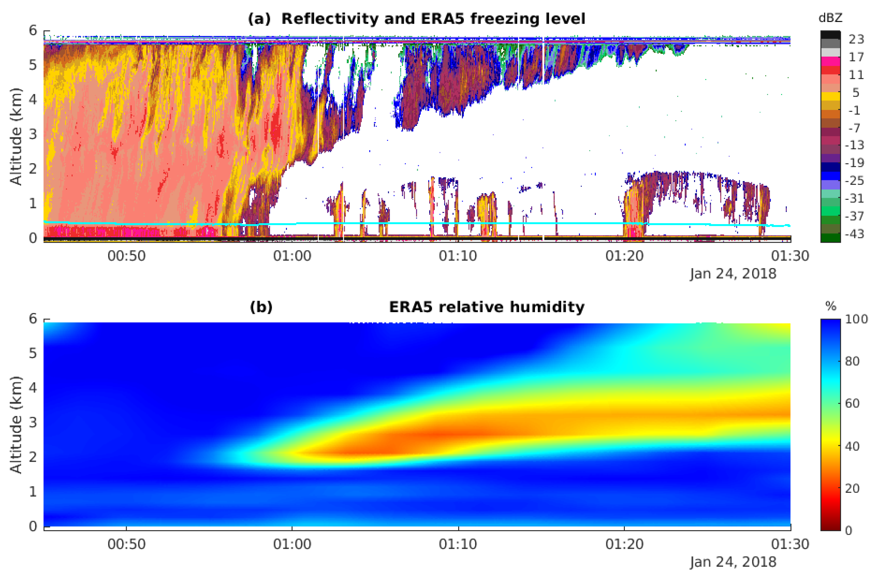
latm in dB multiplied by two (for the transmit and return paths) and adjusted for the incidence angle. Atmospheric attenuation depends on atmospheric pressure, temperature, and relative humidity, and we utilize the ERA5 reanalysis data to calculate
latm using the wave propagation model by the International Telecommunication Union [
21]. For comparison purposes, we also implemented the wave propagation model by [
22], which produced results that were within ~0.2 dB of the ITU results. This comparison provides confidence to the
latm estimate.
3.2.2. Sea Surface Backscatter Modelling
Once the observed
σ0 has been calculated it can be compared to that predicted by an ocean surface backscattering model. When the HCR operates at nadir pointing, quasi-specular scattering theory is applicable, which has been shown to work well for low incidence angles. It gives
σ0 as [
17,
23]:
where
v is the horizontal surface wind speed in m s
−1,
SST is the sea surface temperature in °C,
Γe is the ocean surface effective Fresnel reflection coefficient, and
s(
v)
2 is the surface mean square slope, which is discussed below.
The ocean surface effective Fresnel reflection coefficient is [
17]:
where
Ce is the Fresnel reflection coefficient correction factor, which is given as 0.88 by [
17] for 94 GHz radars. The complex refractive index for sea water
n depends on the wavelength and the sea surface temperature. In theory, it also depends on the salinity of the sea water, but this dependency is very weak so that a constant salinity of 35‰ can be used without loss of accuracy. The dependency on the SST is also relatively weak and therefore the SST is often assumed to be constant, e.g., by [
17,
20]. However, because in our case the HCR has been deployed in areas with vastly different SSTs, from the Caribbean to the Southern Ocean, including the SST dependency in the calculations is desirable. We use the fit for the microwave dielectric constant of sea water by [
24], which is based on microwave satellite observations. Note that [
24] gives the frequency validity range of their fit as only “up to at least 90 GHz”, slightly below the HCR’s 94 GHz.
Several empirical relationships exist for the effective mean square surface slope
s(
v)
2. Cox and Munk [
25] developed a linear relationship with wind speed as:
which was later refined by Wu [
26,
27] and Freilich and Vanhoff [
28] into the following logarithmic relationship:
where
a0 and
a1 are constants with different values derived by different studies in different wind speed regimes, which are listed in
Table 7.
We use
s(
v)
2 by Cox and Munk ([
25], which we will call the CM model), Wu ([
26,
27], the Wu model), and Freilich and Vanhoff ([
28], the FV model), and the complex refractive index for sea water by [
24] to calculate
σ0 with Equation (8). We again use the ERA5 reanalysis data for the U and V surface wind components and for the SST.
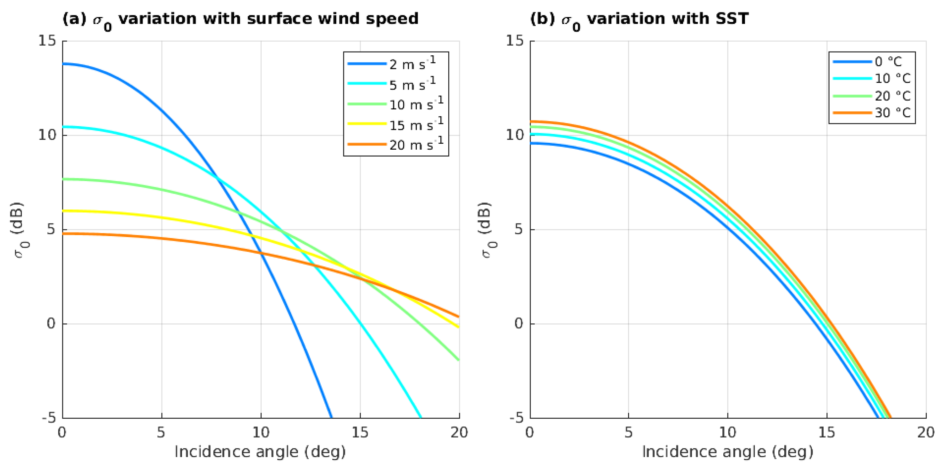
Before we compare the model
σ0 with that calculated from measurements using Equation (7), we investigate how the model
σ0 varies with the surface wind speed and SST. We first vary wind speeds between 1 and 20 m s
−1 while keeping the sea surface temperature constant at 20 °C in the CM model (
Figure 11a) and then keep wind speed constant at 5 m s
−1 while varying the sea surface temperature between 0 and 30 °C (
Figure 11b). The sea surface return values of
σ0 decrease with increasing angles off nadir as the beam is increasingly scattered in directions other than back to the radar receiver. Variations in sea surface temperature shift the curves up and down by a small, but not insignificant amount (up to ~1.5 dB in the 30°C temperature range,
Figure 11b). Varying the surface wind speed, however, changes the slope of the curves significantly (
Figure 11a), where lower wind speeds result in steeper curves and the slope flattens as wind speed increases. These results intuitively make sense when we keep in mind that wind speed is a proxy for wave conditions on the ocean surface. The maximum
σ0 is expected when the beam is perpendicular to the wave surface. The farther the angle deviates from perpendicular, the more the power is reflected in directions other than back towards the receiver. At low wind speeds, representing little or no wave activity, the beam is perpendicular to the ocean surface at nadir pointing, and can therefore be almost completely reflected back to the receiver (specular reflection), but the return power decreases significantly with less perpendicular incidence angles. At higher wind speeds, representing significant wave activity, the slope of the waves determines in which direction the power is reflected. In these circumstances, nadir pointing no longer implies a 90° angle between the beam and the ocean surface and significant portions of the power are reflected out of the receive path. However, at angles pointing off nadir, more of the signal power can be reflected back to the receiver if the beam happens to hit the waves at just the right angle, leading to increased return power, which therefore leads to flatter backscatter curves.
3.2.3. Comparison of Measured and Modelled Sea Surface Backscatter
Comparing modelled and measured
σ0 when pointing directly nadir is not ideal, because uncertainties in the reanalysis wind speeds have the biggest effect at very low incidence angles (
Figure 11a). Wind speed variations seem to have the least effect between 5° and 15° incidence angles (
Figure 11a) and it is therefore desirable to measure
σ0 at these angles. During all three field campaigns sea surface calibration (SScal) events were performed during most flights by scanning the radar ±20° off nadir. This scanning pattern was carried out for at least several minutes at a time.
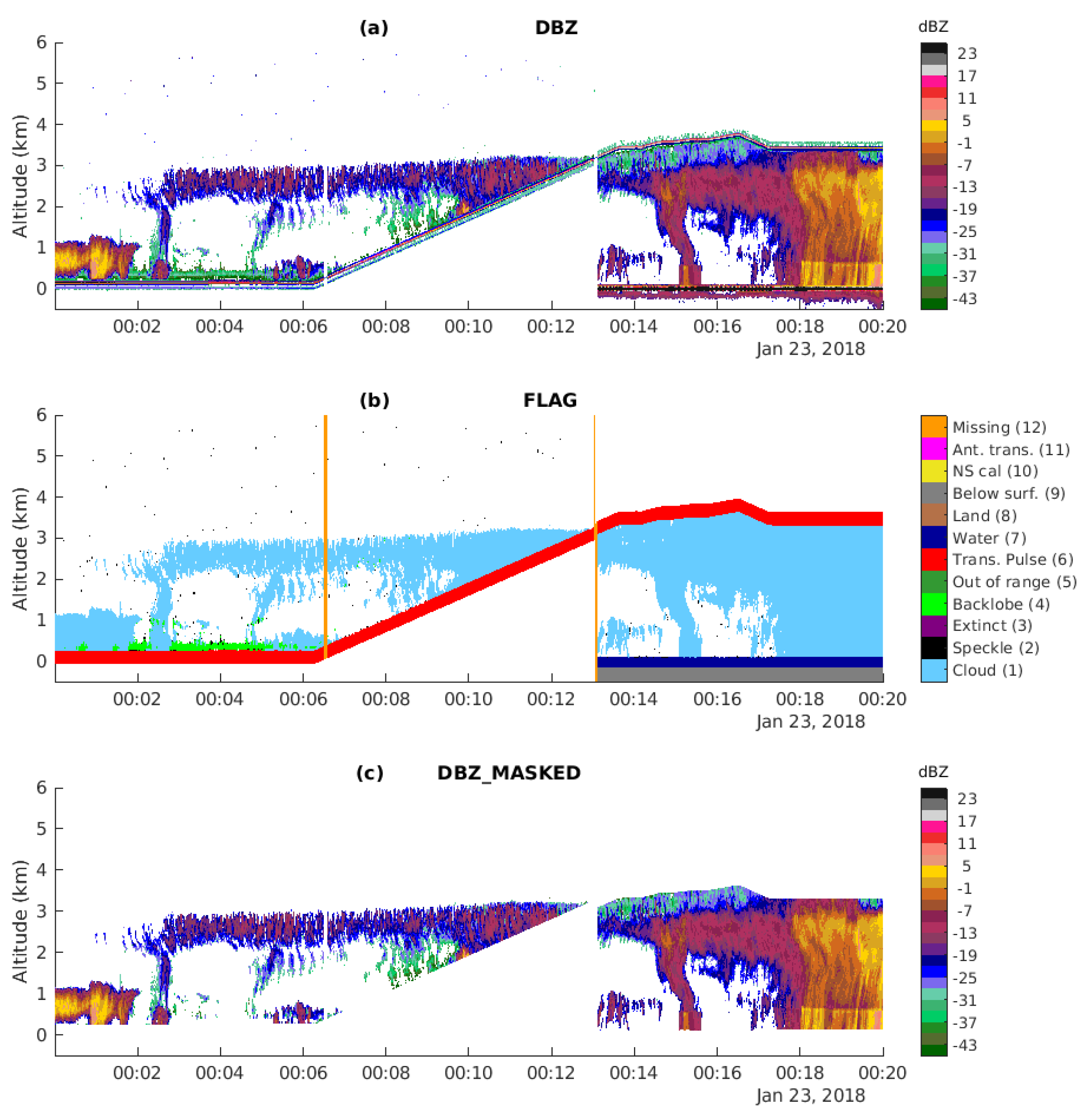
As W-band radars can be heavily attenuated in clouds, care needs to be taken to only use data without cloud contamination. It is up to the radar operator on board the aircraft to determine suitably clear conditions over the ocean. The operator may use down-linked satellite data, the on-board forward-looking camera, or simply check out of the window to determine cloud conditions. Luckily, clear air conditions are also usually the least interesting from a science perspective so that SScal events during these times have little impact on the scientific objectives of the mission. Nevertheless, cloud contamination often occurs so that the first step in the processing of the SScal data is to filter out cloud contaminated data and other unsuitable data. To identify rays that only traverse clear air, we first remove all zenith-pointing rays and times when the aircraft was flying at altitudes less than 2.5 km since the ocean return at low altitudes can be so strong that it saturates the receiver. For the remaining rays we calculate the sum of the reflectivity values in linear space from the aircraft to the first gate identified as ocean surface (
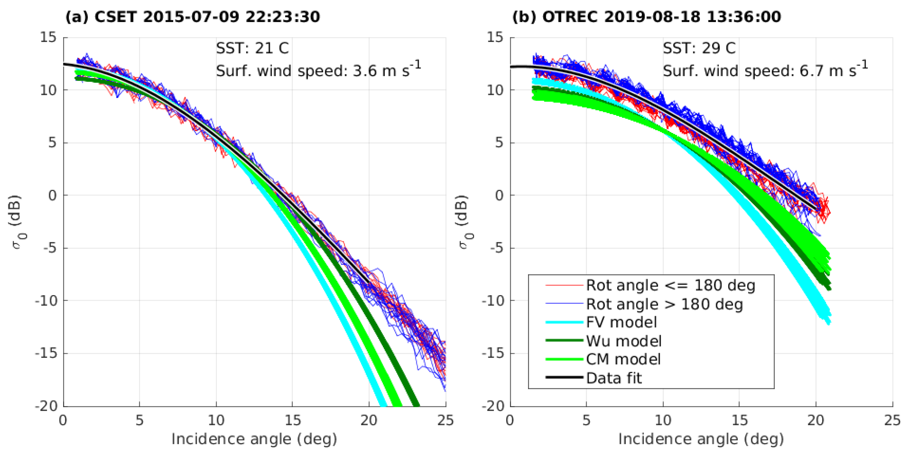
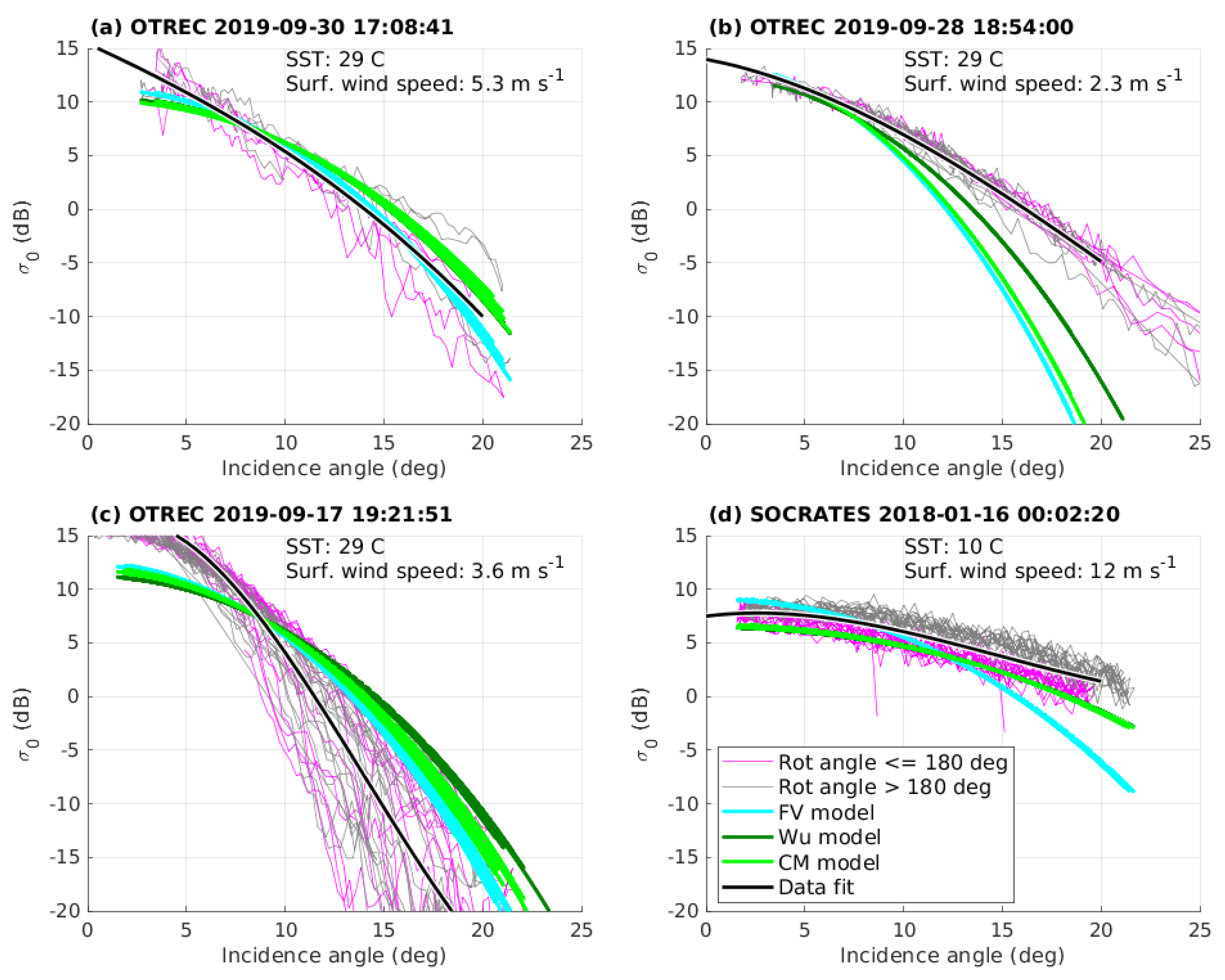
Section 2.3). If the reflectivity sum is larger than a certain threshold (in our case, 0.8 dBZ), we assume that it contains cloud data and exclude it from the SScal analysis. The non-cloud-contaminated results are plotted for each SScal event, along with the three models. Some typical examples are shown in
Figure 12. The red and blue lines show the measured
σ0 as a function of incidence angle while the green lines represent the different models. The black line is a fit through the measurements. Comparing the measurements with the model data gives an estimate of how well the radar reflectivity is calibrated. The ERA5 surface wind speed and SST are shown in the upper right corner.
Even after the removal of cloud-contaminated cases, which is done automatically in our SScal analysis procedure, not all SScal events can be used for calibration. There are several reasons why SScal events may not be suitable: After the removal of cloud contaminated data, sometimes not enough data points remain (
Figure 13a). In some cases, the slope of the measured
σ0 does not agree well with the modelled slope (
Figure 13b). Given the fact that the slope is highly sensitive to varying wind speeds (
Section 3.2.2), we propose that the disagreement between the slope of the measured and modelled
σ0 does not necessarily mean that the radar is not well calibrated, but rather that the reanalysis of the wind speed is not representative of the actual wave conditions. This discrepancy is especially likely near coastlines because the assumption that wind speed is a good proxy for wave conditions may not be valid. SScal events were also not considered when the wind speed is very low and variable within a single event (
Figure 13c). Other SScal events were removed because data measured on one side of the aircraft were distinctly different from data measured on the other side of the aircraft (
Figure 13d). We hypothesize that these distinct measurements were taken under conditions when the aircraft was flying perpendicular to the wave direction, so that the radar scanned the approaching waves on one side and the departing waves on the other side, resulting in different wave slopes with different scattering properties.
After the removal of the non-suitable SScal events, we were left with 27 good events for CSET, 27 for SOCRATES, and 45 for OTREC. Going through the individual plots of each SScal event (not shown) it is evident that the difference between the models and the observations varies between individual events, which is to be expected. Some events show excellent agreement (e.g.,
Figure 12a) while others show a significant bias of sometimes >2 dB (e.g.,
Figure 12b). When the slopes of the measured and modelled
σ0 do agree but the measured curve is shifted up or down as a whole, a bias in the radar calibration is likely. Of course, this up or down shift could also be caused by erroneous sea surface temperatures, but that is rather unlikely because the variations are very small (
Figure 11b). It is interesting to note that there was not a single model that always had the best agreement with the observations. Rather different models performed better for different events, different wind speeds, or different incidence angles. In general, the slopes of the CM and Wu models were similar to each other and agreed somewhat better with the measurements than the FV model.
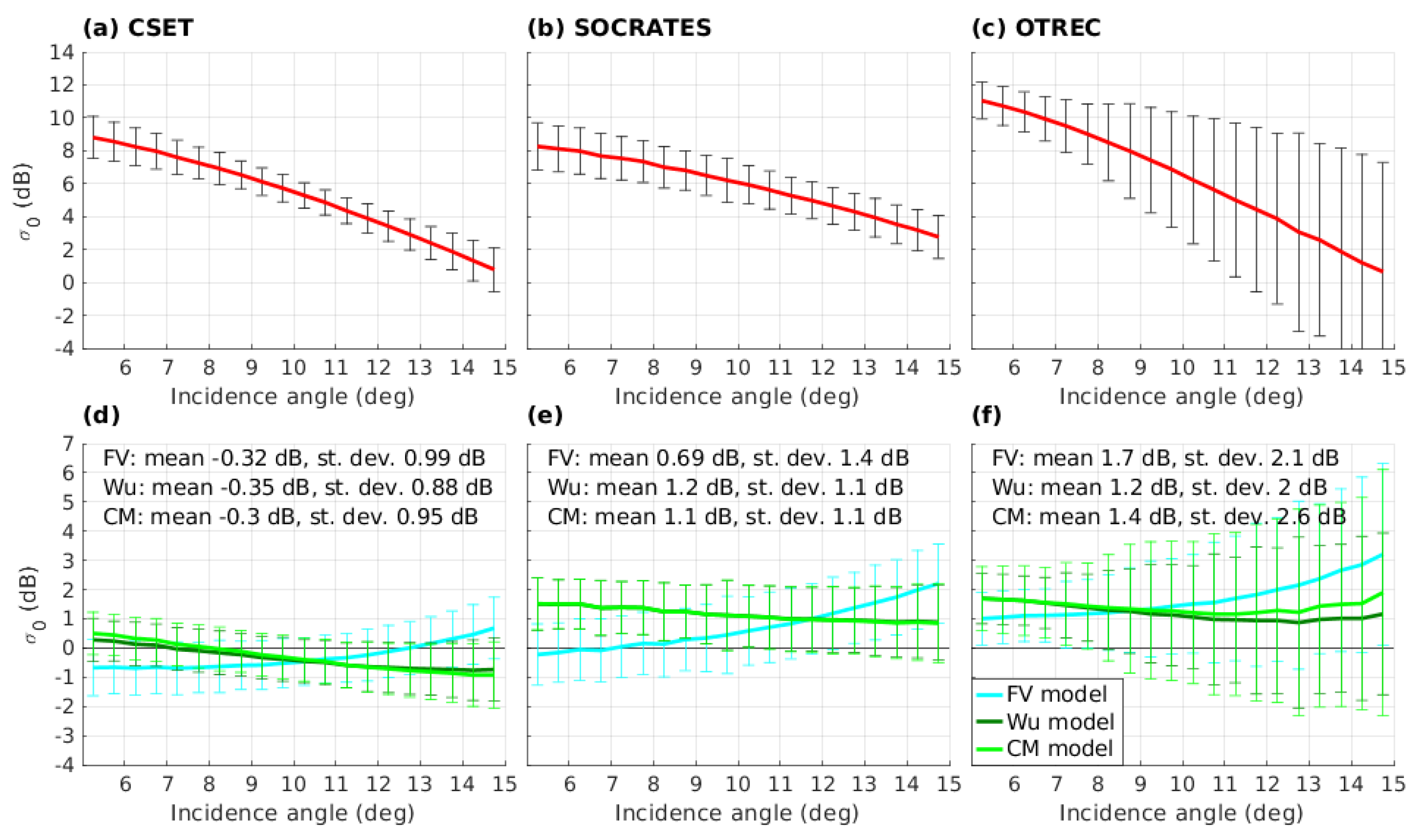
To investigate if we have an overall bias, we first calculate the difference between the measurements and the models for each data point between the incidence angles of 5° and 15° and then calculate the mean and standard deviation of these differences. To summarize the bias at different incidence angles, we collect the data into 0.5° bins and calculate the mean (
Figure 14a–c), mean of the differences (i.e., the bias,
Figure 14d–f), and standard deviations within each bin. Comparing the results from CSET, SOCRATES, and OTREC (
Figure 14), it is evident that the bias curves of the CM and Wu models have mostly a negative slope (except for high incidence angles in OTREC) whereas the FV model has a steeper positive slope (
Figure 14d–f). The steeper slope of the FV model indicates that it is less representative of the HCR measurements than the other two models and therefore we put more emphasis on the CM and Wu models. As a consequence of the different direction of the slopes in the models, the CM and Wu models agree better with the measurements at low incidence angles when the overall bias is negative (as in CSET,
Figure 14f) and high incidence angles when the overall bias is positive (SOCRATES and OTREC,
Figure 14e,f). The opposite is true for the FV model. The ideal model for the HCR is likely somewhere in-between the FV model and the CM/Wu models.
During CSET, we observed a small mean bias of about −0.3 dB with all three models (
Figure 14a). Standard deviations were also low, at less than 1 dB. The good agreement between the measurements and the models, and the low standard deviation can likely be attributed to quite calm conditions during CSET. Wind speeds were low to moderate (not shown) leading to low wave activity in the Pacific. In SOCRATES, the bias was 1.2 dB with the CM and Wu models and 0.7 dB with the FV model (
Figure 14e), with standard deviations of just over 1 dB. Wind speeds were generally very high during SOCRATES, which is reflected in the flat curve of the measured radar cross section (
Figure 14b). The angle between the aircraft track and the waves seems to play a significant role in SOCRATES, as there were several cases where the data measured on one side of the aircraft were distinctly different from data measured on the other side of the aircraft, as shown in
Figure 13d. In OTREC, the overall bias was the largest at 1.4 dB for the CM model, 1.2 dB for the Wu model, and 1.7 dB for the FV model (
Figure 14f). However, the uncertainty in the OTREC results was also the largest, with standard deviations of more than 2 dB (
Figure 14c,f). Two main factors likely play a role in the large uncertainty of the OTREC data: (a) wind speeds were generally low, which is unfavourable as the sensitivity to wind speed deviations is the largest at low wind speeds (
Figure 11a); and (b) many SScal events were carried out close to the coast where the assumption that wind speed is a good proxy for wave conditions is questionable. Overall, the observed biases of around 1–2 dB are very encouraging, and we consider the HCR to be well calibrated. However, the fact that the biases increased between the different field campaigns suggests the need for close attention and is still under investigation.


 ,
, 


