Nowcasting India Economic Growth Using a Mixed-Data Sampling (MIDAS) Model (Empirical Study with Economic Policy Uncertainty–Consumer Prices Index)

Abstract

Economics suffers from a blurred view of the economy due to the delay in the official publication of macroeconomic variables and, essentially, of the most important variable of real GDP. Therefore, this paper aimed at nowcasting GDP in India based on high-frequency data released early. Instead of using a large set of data thus increasing statistical complexity, two main indicators of the Indian economy (economic policy uncertainty and consumer price index) were relied on. The paper followed the MIDAS–Almon (PDL) weighting approach, which allowed us to successfully capture structural breaks and predict Indian GDP for the second quarter of 2021, after evaluating the accuracy of the nowcasting and out-of-sample prediction. Our results indicated low values of the RMSE in the sample and when predicting the out-of-sample1- and 4-quarter horizon, but RMSE increased when predicting the 10-quarter horizon. Due to the effect of the short-term structural break, we found that RMSE values decreased for the last prediction point.

1. Introduction

The official publication of many macroeconomic indicators (such as GDP) has been delayed, especially in developing countries, by Central Statistics Offices. This is a problem for economists and policy-makers who follow the state of the economy. GDP is the most important indicator for policy-makers, and is similar in describing the state of a country’s economy to satellites that describe weather on earth. While meteorologists have today’s weather information and only need to predict tomorrow’s weather, economists need to know today’s information.In the recent past, this has been described as nowcasting. Nowcasting technology allows us to exploit the information in high-frequency data (daily, weekly, monthly) to extract signals about the direction of change in low-frequency data (seasonal, yearly).This technology is only useful in an environment where high-frequency data are issued in real time. Nowcasting is used to generate real-time current GDP estimates as a low-frequency variable (annual, quarterly) based on information from high-frequency variables (monthly, daily) that are released early. Studies [1,2] gave the basis of nowcasting by studying daily GDP developments based on high-frequency data in the US economy. Giannone et al. [3] also developed a method for assessing the marginal impact of monthly data releases that have a jagged edge on current quarter real GDP forecasts. The usual methods used for forecasting rely on dynamic factor models that treat the underlying low-frequency variable of interest as a latent process with high-frequency data observations. These models are inferred using likelihood-based methods and Kalman filtering techniques [4]. Correspondingly, in order to nowcasting GDP, many studies have relied on a large set of high-frequency data using the MIDAS model according to a weighting function that fits the data [5,6,7]

For nowcasting low-frequency variables, researchers rely on a wide range of high-frequency early-release financial economic variables [8]. Among the most frequently used variables are exchange rates, price indices, retail trade, average income [9,10]. Macroeconomics relies on increasingly non-standard data extracted using machine learning (textual analysis) methods, with the analysis involving hundreds of time series. Some studies [11,12] investigated GDP growth forecasting in the U.S.A. using standard high-frequency time series and non-standard data generated by textual analysis of financial press articles and proposed a systematic approach to high-dimensional time regression problems.

In India, there are many studies of nowcasting GDP. Lyer and Gupta [13] used a dynamic factor model to forecast GDP growth in India on a quarterly basis from January 2000 to December 2018. The analysis included 6 quarterly indicators and 12 monthly high-frequency indicators derived from the monetary, financial, and real sectors of India. A work [14] built single-index dynamic factors (DFs) using a sequentially expanding list of 6,9, and 12 high-frequency indicators. Another study [15] used, for nowcasting India’s GDP growth, a dynamic factor model that incorporates a series of USA and Euro zone outputs in order to improve forecasts.A new framework was suggested [14] to forecast India’s Gross Value Added that incorporates information of mixed-data frequencies and other data characteristics. Evening-hour luminosity was added as a crucial high-frequency indicator.

In this paper, we present a framework for the nowcasting of GDP growth in India using a Mixed-Data Frequency Model. Instead of relying on a large number of indicators in forecasting, which often leads to statistical complexity, we relied on two indicators as high-frequency data, in line with the economic theory:first, the economic policy uncertainty index for India [16] as a non-standard indicator based on textual analysis, and second, the consumer price index for India as a standard indicator. The main aim was to assess the extent to which the model is able to anticipate the significant negative effects of the Covid19 pandemic on economic growth in India, as most statistical models collapse during crises (global financial crisis) [17]. Studying the effects of uncertainty on India’s economic growth is difficult because, as far as we know, these effects have not been studied before. At the same time, the proposed model provides real-time GDP growth nowcasting and continuous updates to the GDP growth in India, given that the data of Economic Policy Uncertainty index and Consumer Price Index are issued in real time, which gives a great benefit to trackers of the state of the economy.

2. Materials and Methods

The term MIDAS refers to regression analysis by sampling data measured at different frequencies. As a remedy to the problem of variation in statistical versions in economics, the methodology [18,19,20] addresses the situation where the dependent variable in the regression is sampled at a lower frequency than that of one or more of the regressors. The aim of the MIDAS approach is to incorporate the information present in the higher frequency data into the lower frequency regression in a parsimonious, yet flexible, fashion. An additional advantage of these models is that some additional value for the high-frequency variables may be available after observing the latest value of the low-frequency dependent variable sample. In this case, these additional observations can be used to update the predictions, which is called nowcasting. The following is the general form of the MIDAS regression equation:

$$Y_t=\beta X_t+{\displaystyle \sum }_{p=0}^{S-1}{X}_{\left(t-p\right)/S}^H{\theta }_p+{\epsilon }_t$$

(1)

where $Y_t$ is the variable low frequency during the period (t), $X_t$ isthe set of regressors sampled at the same low frequency $Y_t$,$X_{\left(t-p\right)/S}^H$ idthe set of regressors sampled at a higher frequency with $S$ values for each low-frequency value, $p$ isthe high-frequency lag at t, $\theta$ indicates the partial effect parameters for each frequency interval $S$, and ${\epsilon }_t$ is the error term.

This approach estimates a distinct $\theta$ for each $S$ high-frequency lag regression. The MIDAS model estimation provides various weighting functions that reduce the number of parameters in the model by placing constraints on the effects of high-frequency variables to suit their properties and according to some assumptions.

2.1. Step Weighting

According to this function, the notation of Equation (1) becomes as follow [19]:

$$Y_t=\beta X_t+{\displaystyle \sum }_{p=0}^{k-1}{X}_{\left(t-p\right)/S}^H{\theta }_p+{\epsilon }_t$$

(2)

where $k$: is the number of lagged high frequency, and $p$ is the step length; the number of high-frequency coefficient increases with the number of lags. A linear trend between the variables is preferred when using this function.

2.2. Almon (PDL) Weighting

For each high-frequency lag up to $k$, the regression coefficient is modeled as a $q$ dimensional lag polynomial in the MIDAS parameters $\theta$. Equation (1) follows [19]:

$$Y_t=\beta X_t+{\displaystyle \sum }_{p=0}^{k-1}{X}_{\left(t-p\right)/S}^H{{\displaystyle \sum }}_{j=1}^q{p}^j{\theta }_j+{\epsilon }_t$$

(3)

where $q$ is the almon polynomial order and the chosen number of lag $k$. This function isused if the data have multiple trends (quadratic, cubic).

2.3. Beta Weighting

Ghysels et al. [19] suggest a normalized beta-weighting function, according to the equation:

$$Y_t=\beta X_t+{\displaystyle \sum }_{p=0}^{k-1}{X}_{\left(t-p\right)/S}^H\left(\frac{i_L{}^{{\lambda }_1-1}{\left(1-i_L\right)}^{{\lambda }_2-1}}{{{\displaystyle \sum }}_{j=0}^k{i}_j^{{\lambda }_1-1}{\left(1-i_j\right)}^{{\lambda }_2-1}}+{\lambda }_3\right)\gamma +{\epsilon }_t$$

(4)

where ${\lambda }_1, {\lambda }_2, {\lambda }_3$ are hyperparameters governing the shape of the weighting function, $\gamma$ is a slop coefficient that is common across lags, $kand$ is the number of lags. This function can be used when the shape of the distribution of the variables is unknown or distorted.

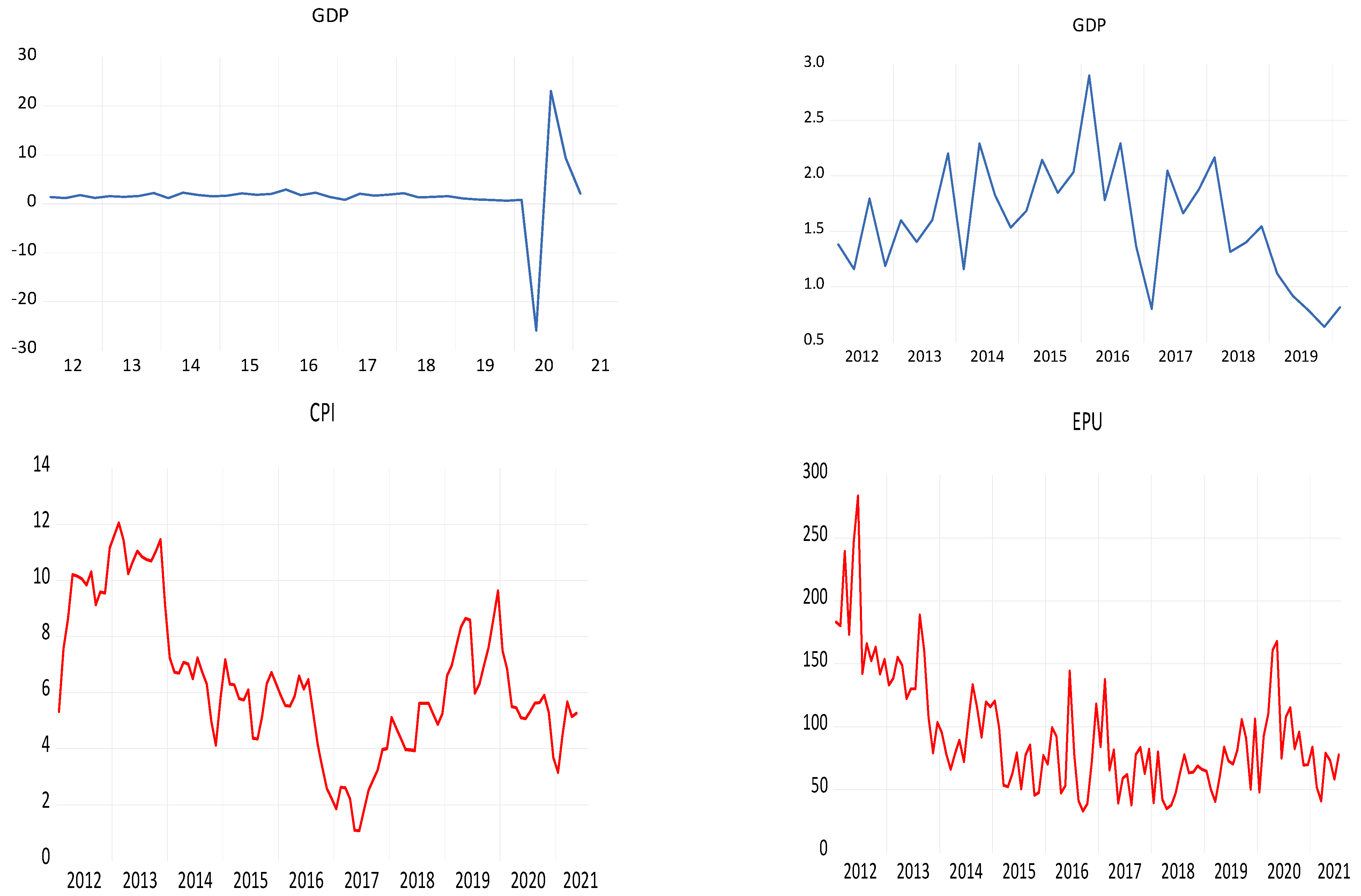
3. Data and Theory

Our efforts for nowcasting real GDP growth in India as a low-frequency variable were based on the quarterly data available in the Federal Reserve Economic Data database from 2012 through the first quarter (Q1) of 2021. For the high-frequency (monthly) variables as independent variables, we used the India economic policy uncertainty index as a proxy for the non-standard indicators calculated according to a previously reported methodology [16]. The data are available from 2012 to July 2021 on the website [21]. The index is based on newspaper articles. Seven Indian newspapers are included: The Economic Times, The Times of India, the Hindustan Times, the Hindu, The Statesman, The Indian Express, and The Financial Express. The news articles containing at least one of the terms indicative of economic policy uncertainty were counted and classified into three groups: the first group included uncertain, uncertainties, or uncertainty. The second group included economic or economy. The third category included policy terms such as regulation, central bank, monetary policy, policymakers, deficit, legislation, and fiscal policy. The monthly Economic Policy Uncertainty article count was reduced by subtracting the number of all articles in the same newspaper and month. Each paper-specific series was normalized to standard deviation 1 prior to 2011. Once normalized, the seven newspaper-specific indices were then summed. The resulting series was normalized to mean 100 prior to 2011. Empirical studies [16,22,23,24,25,26] have confirmed that high levels of uncertainty lead to a slowdown in economic growth. Whereas uncertainty can lead companies to postpone hiring decisions, it affects workers’ decisions, making them less willing to search for job opportunities, and it accompanies high volatility in macroeconomic variables, which makes the economic policy uncertainty index capture the slowdown in India’s economic growth. The second high-frequency indicator as a standard index that we considered was the consumer price growth (inflation rate, total of all items) of India during the monthly period from 2012 to June 2021, drawn from the Federal Reserve Economic Data database. The rise in consumer prices can be a driver of economic growth and can have a negative impact on economic growth. Large and continuous rises in prices could lead to a decrease in the return on capital and weak real spending, which leads to a decrease in the confidence of investors and consumers in the economy and thus a decrease in growth. On the other hand, if price growth is controlled at acceptable levels, real consumer spending will increase, and thus the economy will achieve expulsion growth. Accordingly, the importance of these indicators is reflected in the current and future forecast of the trends of the Indian economy.

4. Methodology

With our methodology, for nowcasting the Q2 of 2021 of India’s economic growth, we divided the GDP growth data in India into two sets: the data from Q1 of 2012 toQ4 of 2018 for training, and the data from Q1 of 2019 to Q1 of 2021 to test the validity of the forecasts and the model ability for the nowcasting of developments in economic growth in India during 2019 and 2020.

Accordingly, our methodology included several stages. To visualize the data features (patterns, unusual observations, changes over time), we first plotted the data, then translated them with descriptive statistics and the normal distribution of the data using the following statistic:

$$Jarque-Bera=\frac{n}{6}\left(S^2+\frac{1}{4}{\left(K-3\right)}^2\right)$$

(5)

where $n$ is the number of observations, $S$ is skewness, $K$ is kurtosis.Because most economic variables show a stochastic trend and may be exposed to shocks that do not allow them to return to their pre-shock average, economic time series may undergo discrete changes at a particular date or gradual changes over time called “breaks”, often associated with economic policy or structural changes in the economy. We need to study the extent to which these variables are affected by using the Breakpoint Unit Root test previously proposed [27,28,29,30]. Assuming that breaks follow the dynamic course of innovations, we tested the stationarity of our variables according to the following equation:

$$y_t=c+\alpha t+\theta D{U}_t\left(T_b\right)+\gamma D{T}_t\left(T_b\right)+\omega D_t\left(T_b\right)+\delta y_{t-1}+{\displaystyle \sum }_{i=1}^p{\phi }_i\Delta y_{t-i}+{\epsilon }_t$$

(6)

where $\alpha , \theta , \gamma , \omega$ are trend and break parameters, $c$ is a constant, $p$ is the lag order of the autoregressive process.The test was carried out under the null hypothesis $\delta =0$ (not stationary with or without break) against the alternative of $\delta <0$ (stationary with or without break). In the next step, in order to avoid the problem of multicollinearity, we tested the degree of a linear relationship between the high-frequency independent variables, which was obtained according to:

$$r=\frac{\sum X_1{X}_2-n\overline{X_1}\overline{X_2}}{\left(n-1\right)\ast {\sigma }_{X1}{\sigma }_{X2}}$$

(7)

where $X_1, X_2$ are independent variables, ${\sigma }_{X1}, {\sigma }_{X2}$ indicatethe standard deviation. With no multicollinearity problem, we estimated the MIDAS model for nowcasting the Q2 of 2021 and used the fourth-degree Almon PDL weighting for capturing volatility in the data and giving an appropriate slowdown period for each high-frequency variable according to the Akaike Information Criterion (AIC), which is given as follow [31]

$$-2log L\left(\widehat{\theta }\right)+2k$$

(8)

where $\widehat{\theta }$ is the maximum value of the likelihood function, $k$ is thenumber of variables. We also included in the model the AR(p) term for the low-frequency variable in order to benefit from the historical information of the variable in addition to the information of the high-frequency variables in forecasting, which is an advantage for these models (AR-MIDAS) over the dynamic factor model. After estimating the model, we evaluated the model forecast ability by testing the random error term ${\epsilon }_t$: the error term values must be distributed in a normal distribution, according to the testing Equation (5). In addition, the error term values should not be self-correlated; we tested this using the auto correlation function:

$$\rho \left(p\right)=\frac{Cov\left({\epsilon }_t,{\epsilon }_{t+p}\right)}{{\sigma }^2}$$

(9)

where $p$ is the number of lags. The random error term series must be stationary, and we tested this with the augmented dickey fuller (ADF) equation [32]:

$$\Delta {\epsilon }_t=c+\alpha .t+\delta {\epsilon }_{t-1}+{\beta }_{p-1}\Delta {\epsilon }_{t-p+1}$$

(10)

where $c$ is a constant, $\alpha$ is a coefficient on a time trend, $p$ is the lag order of the autoregressive process. The ADF test was carried out under the null hypothesis $\delta =0$ (not stationary) against the alternative hypothesis of $\delta <0$ (stationary). After obtaining the predictions, the accuracy of the predictions was confirmed in- and out-of-sample and on the short and long term, depending on Root Mean-Square Error (RMSE):

$$\sqrt{\frac{{{\displaystyle \sum }}_{\mathrm{t}=1}^{\mathrm{n}}{\left(\widehat{{\mathrm{y}}_{\mathrm{t}}}-{\mathrm{y}}_{\mathrm{t}}\right)}^2}{\mathrm{n}}}$$

(11)

where $\widehat{{\mathrm{y}}_{\mathrm{t}}}$ is the forecast value, $y_t$ is the actual value, $n$ is the number of fits observed. The closer the value of this indicator is to zero, the more expected values are identical to the actual one [33].

5. Empirical Results

We created a monthly (high-frequency) visualization of India’s quarterly real GDP growth, economic policy uncertainty (EPU), and consumer price rate (CPI).As an advantage over the literature reviews that used nowcasting models, the use of indicators of uncertainty and consumer prices may provide important and quick results in picking up signals of change in GDP growth, but because of the overlapping patterns and factors affecting GDP growth, the use of only two variables is a limit that affects the nowcasting results. Figure 1 shows that the margin of GDP volatility before 2020 (Stationary) was less than afterwards; it was the largest, at 2.9%, in 2016 Q1 and the lowest, at 0.8%, in 2017Q1. Then, there was a sharp decline in 2021 Q2 at a rate of −26%. This was due to the effects of the COVID-19 pandemic and the great leap achieved by the economic growth during the third quarter of 2021, driven by the decline in the quarter before it [22,23,24,25,26,27,28,29,30,31,32]. This made forecasting of the growth rate more difficult, especially after the second wave of the COVID-19 pandemic. Figure 1 also shows that the largest increase in consumer prices, which reached 2013 M2, was due to the increase in the prices of vegetables and fruits. We also note that the growth rate of consumer prices took an upward trend from the beginning of 2018 until the end of 2019 and remained at high levels during the subsequent period due to the rise in prices in various economic and health sectors. We note from Figure 1 that the economic policy uncertainty index reached high levels in 2012 and 2020.

The data visualization shows that when (EPU) (CPI) rises, GDP falls, and thus our current 2021 Q2 forecast suggests an improvement. The following table reports the most important descriptive statistics and normal distribution of the variables:

The

Table 1. Descriptive statistics and normal distribution of the variables.

Variables	Normality	Mean	Standard Deviation	Maximum	Minimum	Skewness	Kurtosis
	J-B
GDP%	343.6 ***	1.64	5.98	23.12	−25.29	−1.39	17.66
EPU	61.6 ***	94.09	46.82	283.68	32.88	1.37	5.31
CPI%	2.89	6.37	2.57	12.06	1.08	0.32	2.54

*** Indicates significance at 1%. ** significance at 5%. * significance at 1%.

shows that both GDP growth and economic policy uncertainty are not distributed according to the normal distribution. Considering GDP, the large difference between the maximum and the minimum values that occurred during 2020 caused the distribution to become significantly kurtosis and skewed to the left with strongly negative growth. We also note the significant difference between the maximum (283.68) and the minimum (32.88) values of the EPU index, which occurred in 2012M6 and 2016M6, respectively. This also led to a high kurtosis greater than 3 (normal). We notice that the outlier value in 2012M6 skewed the distribution to the right. As for the CPI rate, the data present a normal distribution, and the average during the studied period was 6.73% with a standard deviation of 2.37, which indicates am increase in price in general for the study period [19,20,21,22,23,24,25,26,27,28,29,30,31]. To find the extent of the impact of these values on the variable, we used the Breakpoint unit root test and obtained the following results.

Table 2. Breakpoint Unit Root Test for GDP.

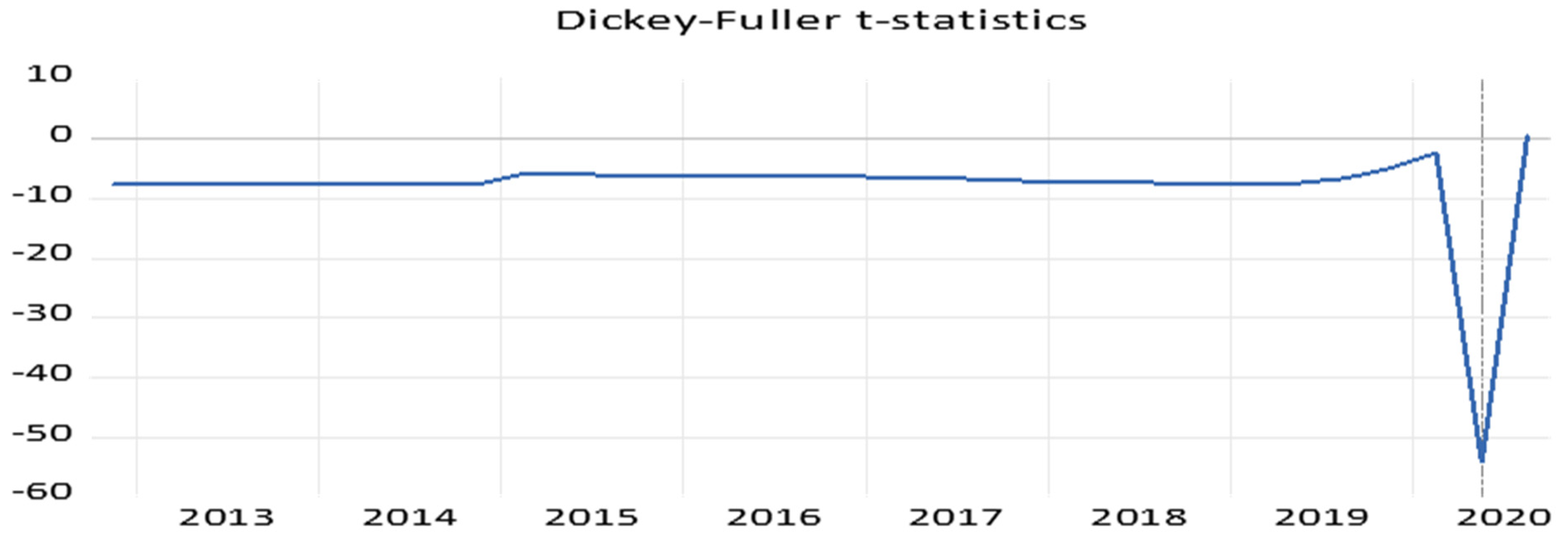
GDP	Stationary	GDP (−1)	C	TREND	INCPT BREAK	TREND BREAK	BREAKDUM	Integrated
t-statistics	−54.25 ***	−4.9 ***	10.76 ***	−1.97 *	23.23 ***	−16.95 ***	−46.80 ***	I(0)
Break Date	2020 Q2

*** Indicates significance at 1%. ** significance at 5%. * significance at 1%.

shows that the date of 2020 Q2 was set as a point of structural break.We determined the significance of all parameters of the model. The break occurred at the intercept and trend levels. We also found that t-statistics stationary is significant at 1%, and therefore, we concluded that the point structural break caused a short-term change in GDP and was stationary at that level. To complete our steps before building the model, we estimated the correlation matrix for high-frequency variables to make sure that there was no multicollinearity.

The results of the correlation matrix estimationshowed that the degree of linear correlation (0.544) was low among the variables, and thus we ruled out a problem of multicollinearity. We then built the model and obtained the following results, presented in

Table 3. Residuals test results.

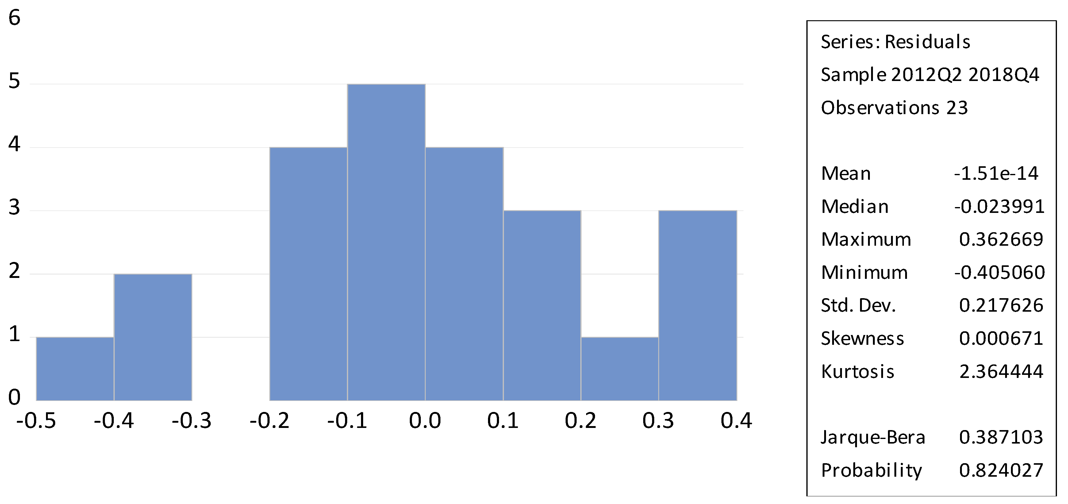
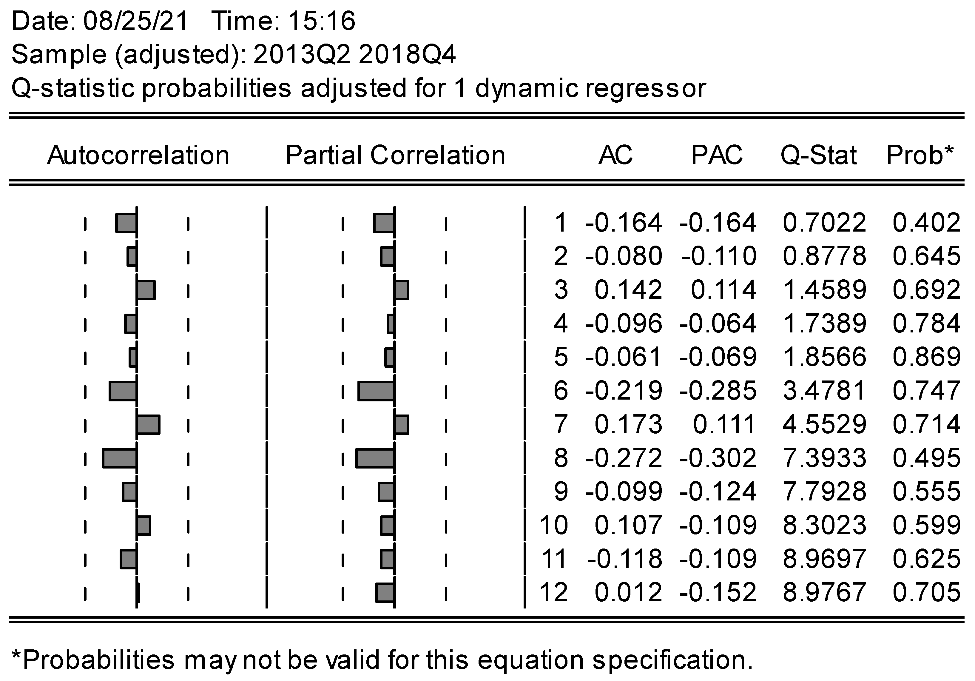
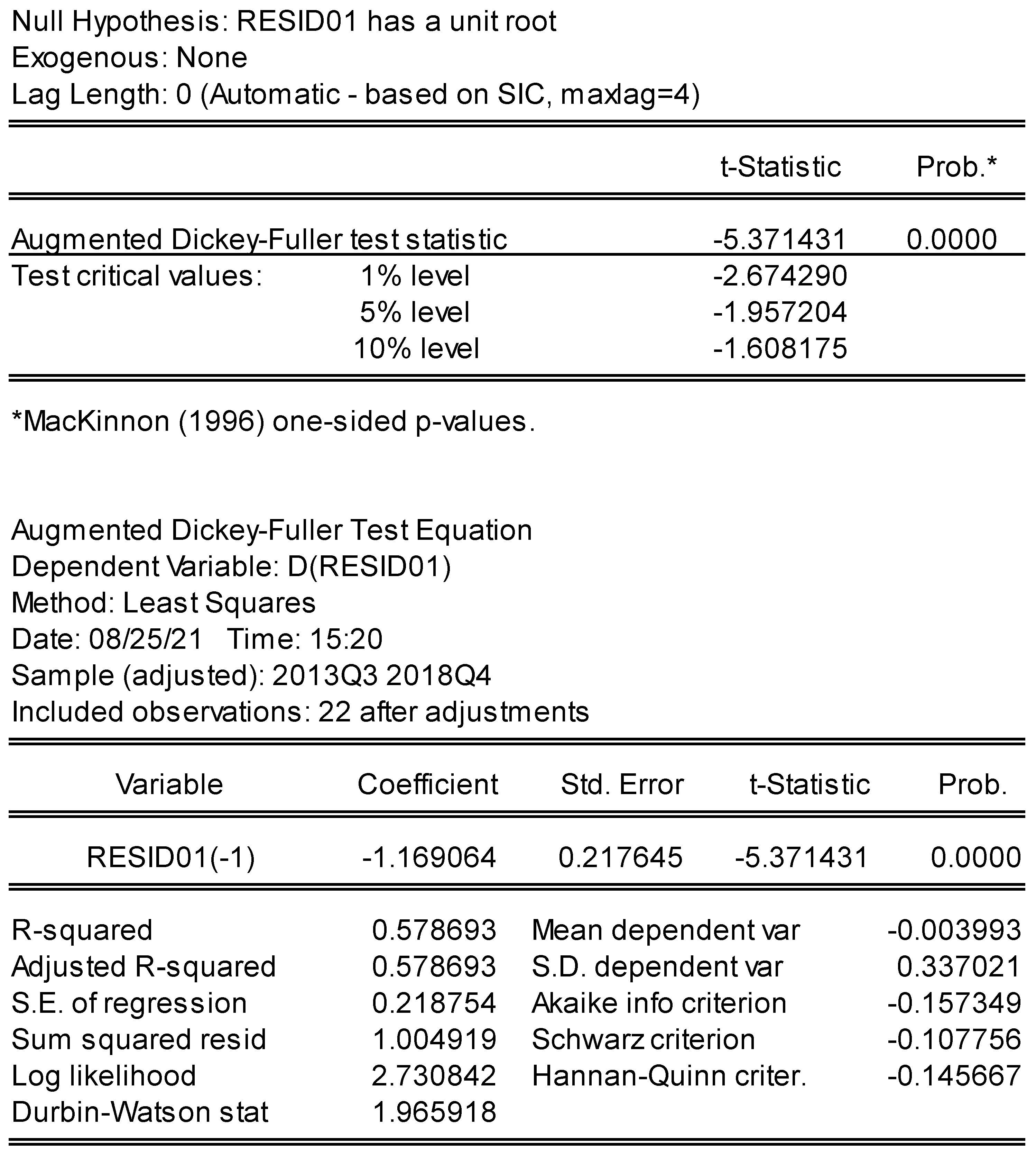
Test	Normality	ACF2	ADF
	J-B		Non Constant–Non Trend
Residuals (PROB)	0.824	0.645	000 ***

*** Indicates significance at 1%. See Appendix A for statistical details.

, divided into three main sections. The first section represents the AR (1) equation for the low-frequency variable. We note the significance of the parameters and the negative impact of GDP on their previous values. The second and third sections show the polynomial coefficient for high-frequency variables. We note that two lag periods were subtracted from high-frequency variables, since we needed two months out of each quarter to predict the low-frequency variable. Table 3 shows that 5 lag periods were selected for EPU, and 15 lag periods were chosen for CPI according to the AIC that achieved the least values for model sum of squared residuals (Figure 2). We note the significant effect of the partial coefficient of the monthly variables in each quarter of GDP.

Table 4. Estimation using Mixed-Data Sampling.

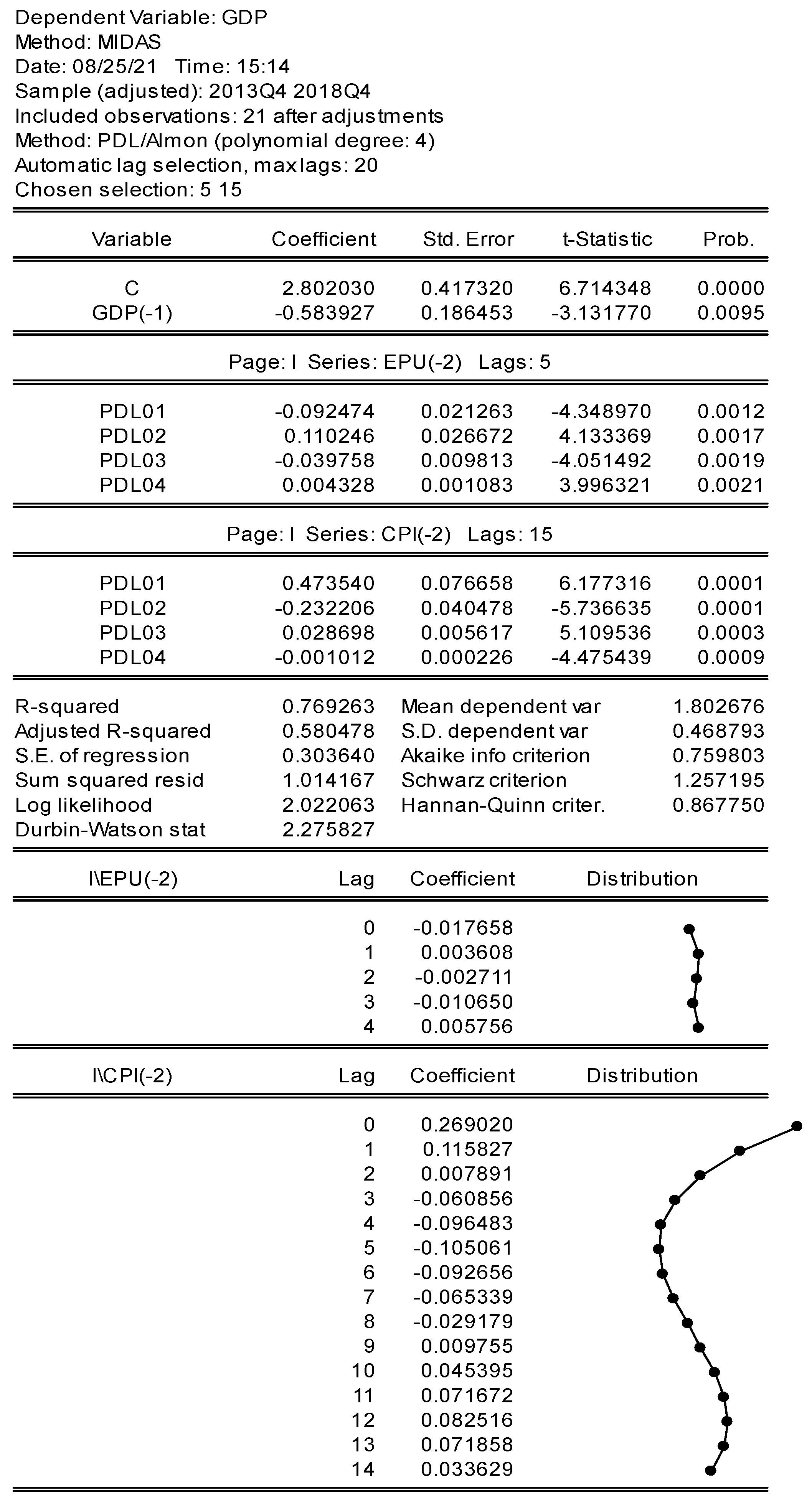
Dependent Variable: GDP (2013Q4 2018Q4)
Variable	Coefficient	Std. Error	t-Statistics
C	2.80203	0.41732	6.714348 ***
GDP (−1)	−0.583927	0.186453	−3.131770 ***
EPU(−2) Lags: 5
PDL1	−0.092474	0.021263	−4.348970 ***
PDL2	0.110246	0.026672	4.133369 ***
PDL3	−0.039758	0.009813	−4.051492 ***
PDL4	0.004328	0.001083	3.996321 ***
CPI(−2) Lags: 15
PDL1	0.47354	0.076658	6.177316 ***
PDL2	−0.232206	0.040478	−5.736635 ***
PDL3	0.028698	0.005617	5.109536 ***
PDL4	−0.001012	0.000226	−4.475439 ***
Adg. R-Squared	0.580478	Log Likelihood	2.022063

*** Indicates significance at 1%. ** Significance at 5%. * Significance at 1%.

shows that the effects of EPU varied but had a negative impact on the growth of GDP in each quarter, while the impact was positive for the growth of CPI (see Appendix A). The Durbin Watson stat indicates no first-order autocorrelation between the residuals [19,29]. Here, we needed to test autocorrelation between residuals of more than one degree, due to the use of lags.

Before issuing nowcasting, we checked that the standard assumptions for the residuals were correct:

The results showed that the residuals were distributed according to a normal distribution, and we noted that there was no autocorrelation between different orders.We found that the residual series was stationary. Now, according to the previous results, we performed multi-step ahead nowcasting to forecast 2021 Q2 and obtained the following results.

The visual representation showed (Figure 3) that the expected values using the model were close to the actual data points. The most prominent observation is that the model succeeded in capturing the point of structural change in 2020 Q2, but not the actual value that it reached, as indicated in Figure 4.

The presence of such large changes makes any statistical model invalid, but our model accurately predicted when the structural Break would occur. We calculated the RMSE (

Table 5. Evaluating the performance of the model in and out of sample.

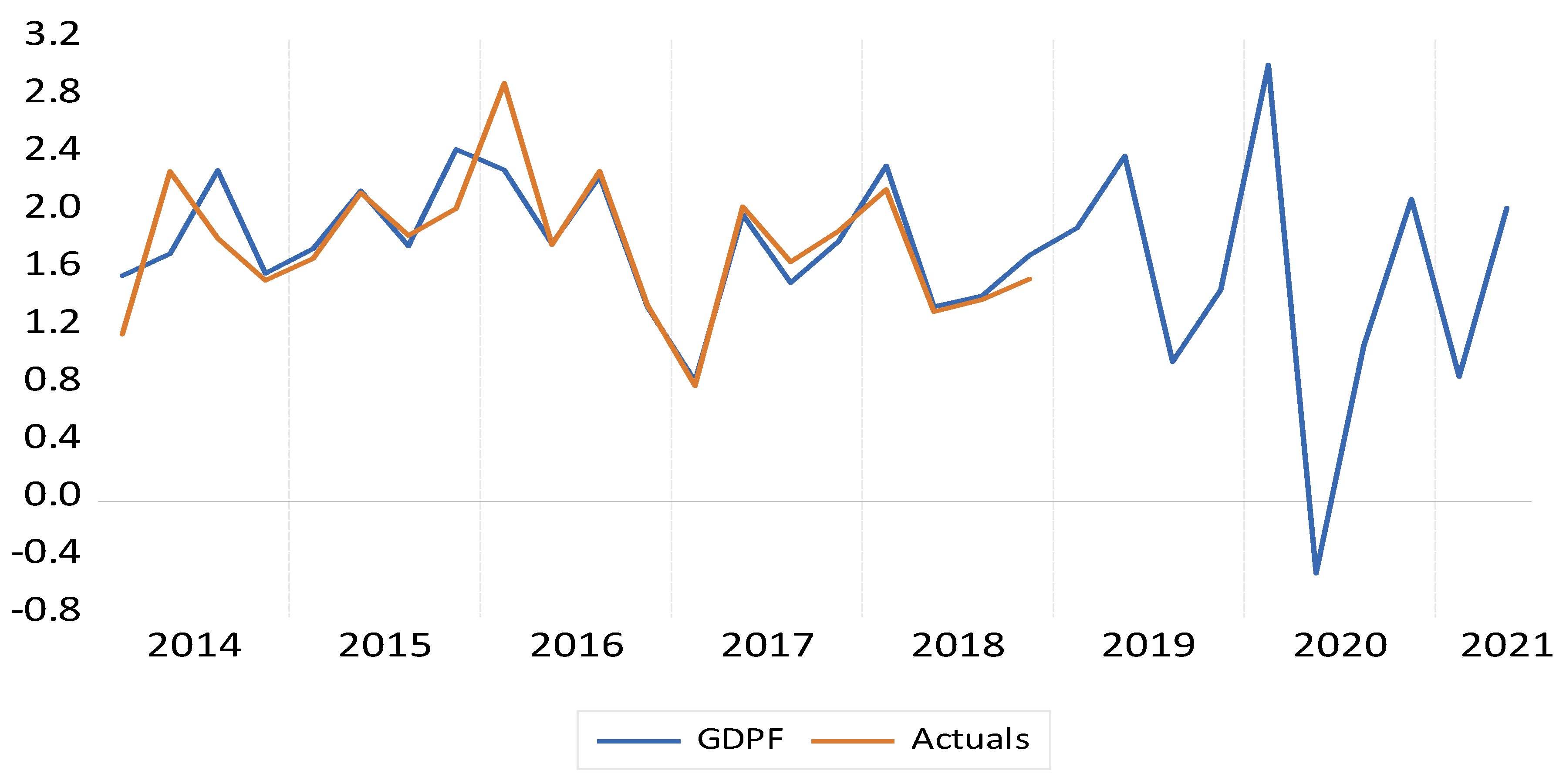
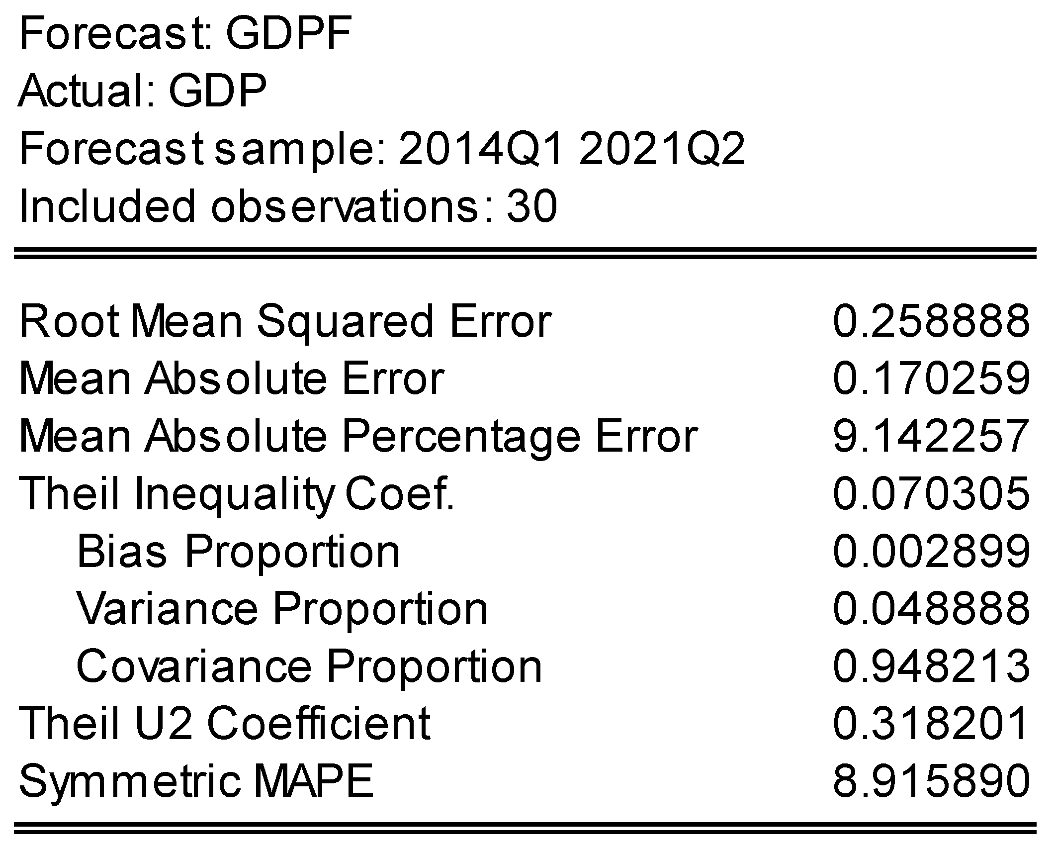
	In of Sample (Training Data)	Out of Sample (Testing Data)
Horizon (Quarter)		H = 1	H = 4	H = 10	H = Last Point
RMSE	0.258	0.778	0.937	11.51	1.24

) to evaluate the predictions in and out of sample on the horizon (short, medium, long):

We see from the table that RMSE values [32] were less than 1 for in-sample forecasting, the model achieved satisfactory results for out-of-sample forecasting at the horizons of 1 and 4 quarters, and the RMSE value became large for forecasting during 2020, as the value included the structural break that GDP growth was exposed to during 2020, but the results of Table 2 show that the structural break was short-term, as the model achieved a lower value of RMSE at the last forecast point. According to our expectations that GDP growth will achieve 2.1% in 2021 Q2, affected by an increase in CPI and a decrease in EPU, we were able to include in the forecast the month of July, in which the level of the index increased, which might herald a new decline in 2021Q3.It is possible to include any new data for indicators and update the forecasting based on that. This model can also be used to understand the effect of targeting a variable on GDP growth. For example, suppose that the economic policy in India aims to stabilize the CPI (i.e., zero growth) for the next three months. This information can be included in the model and obtain GDP growth forecasts for the third quarter; this indicated a drop in growth of −0.64%.

6. Conclusions

This paper presents a framework for nowcasting India’s GDP using the MIDAS–Almon (PDL) weighting model, relying on the information in high-frequency data, instead of including a large number of variables that lead to statistical complexity. Two indicators were relied on, namely, Economic Policy Uncertainty (EPU) for India as a proxy for non-standard indicators and the Consumer Price Index (CPI) as a proxy for standard indicators. The model showed a negative effect of EPU and a positive effect of CPI on GDP growth, as high periods of EPU correspond to a decrease in GDP growth, and high periods of CPI correspond to a rise in GDP growth in accordance with the economic theory. In addition to the information in the high-frequency variables, we made use of the historical information in the low-frequency variable and performed the estimation on the training data. The prediction results showed low values of the RMSE in the sample and when predicting the 1- and 4-quarter horizon for out of sample, but the RMSE increased when predicting the 10-quarter horizon. Due to the effect of a short-term structural break, we found that the RMSE values decreased for the last prediction point. The nowcasting results indicated that GDP growth will achieve 2.1% in 2021 Q2, affected by an increase in CPI and a decrease in EPU. Compared with the results of the literature reviews for nowcasting India GDP growth, the models previously used did not allow capturing the structure break in GDP growth during the COVID-19 pandemic, despite the large number of high-frequency variables used, which suggests that future studies should include EPU when nowcasting changes in India GDP growth. This exercise is expected to be useful to India’s economic planners and policy-makers in institutions and sites that are concerned with economic forecasts for the present and the near future of economic growth, which can be obtained with specific constraints.

References

- Ghysels, E.; Horan, C.; Moencch, E. Forecasting through the rearview mirror: Data revisions and bond return predictability. Rev. Financ. Stud. 2018, 31, 678–714. [Google Scholar] [CrossRef]
- Evans, M. Where Are We Now? Real-Time Estimates of the Macroeconomic. Int. J. Cent. Bank 2005, 1, 127–175. [Google Scholar]
- Giannone, D.; Reichlin, V.; Small, D. Nowcasting: The real-time informational content of macroeconomic data. J. Monet. Econ. 2008, 55, 665–676. [Google Scholar] [CrossRef]
- Banbura, M.; Giannone, D.; Modugno, M.; Reichlin, L. Now-casting and the real-time data flow. In Handbook of Economic Forecasting; Elsevier: Amsterdam, The Netherlands, 2013; Volume 2, pp. 195–237. [Google Scholar]
- Olli-Matti, L.; Annika, L. Nowcasting Finnish GDP Growth Using Financial Variables: A MIDAS Approach; BoF Economics Review; Bank of Finland: Helsinki, Finland, 2020. [Google Scholar]
- Gunay, M. Nowcasting Turkish GDP with MIDAS: Role of Functional Form of the Lag Polynomial; Working Paper; Central Bank of the Republic of Turkey: Ankara, Turkey, 2020. [Google Scholar]
- Barsoun, F.; Stankiewicz, S. Forecasting GDP Growth Using Mixed-Frequency Models with Switching Regimes; Working Paper Series; University of Konstanz: Konstanz, Germany, 2013. [Google Scholar]
- Jardet, C.; Meunier, B. Nowcasting World GDP Growth with High-Frequency Data; Working paper; Banque de France: Paris, France, 2020. [Google Scholar]
- Rufino, C.C. Nowcasting Philippine Economic Growth Using MIDAS Regression Modeling. DLSU Bus. Econ. Rev. 2019, 29, 14–23. [Google Scholar]
- Bok, B.; Caratelli, D.; Giannone, D.; Sbordone, A.M.; Tambalotti, A. Macroeconomic Nowcasting and Forecasting with Big Data. Annu. Rev. Econ. 2018, 10, 615–643. [Google Scholar] [CrossRef] [Green Version]
- Thorsrud, L.A. Words are the New Numbers: A Newsy Coincident Index of the Business Cycle. J. Bus. Econ. Stat. 2018, 38, 393–409. [Google Scholar] [CrossRef]
- Babii, A.; Ghysels, E.; Striaukas, J. Machine Learning Time Series Regressions with an Application to Nowcasting. J. Bus. Econ. Stat. 2021, 1–23. [Google Scholar] [CrossRef]
- Lyer, T.; Gupta, S. Nowcasting Economic Growth in India: The Role of Rainfall; ADB Economics Working Paper Series; Asian Development Bank: Mandaluyong, Philippines, 2019. [Google Scholar]
- Bhadury, S.; Ghosh, S.; Kumar, P. Nowcasting Indian GDP Growth Using a Dynamic Factor Model; Reserve Bank of India: Mumbai, India, 2020. [Google Scholar]
- Bragoli, D.; Fosten, J. Nowcasting Indian GDP. Oxf. Bull. Econ. Stat. 2018, 80, 259–282. [Google Scholar] [CrossRef] [Green Version]
- Baker, S.R.; Bloom, N.; Davis, S.J. Measuring Economic Policy Uncertainty. Q. J. Econ. 2016, 131, 1593–1636. [Google Scholar] [CrossRef]
- Ghysels, E.; Pedro, S.; Rossen, V. The MIDAS Touch: Mixed Data Sampling Regression Models; University of North Carolina and UCLA Discussion Paper; 2004; Available online: https://rady.ucsd.edu/faculty/directory/valkanov/pub/docs/midas-touch.pdf (accessed on 13 October 2021).
- Ghysels, E.; Pedro, S.; Rossen, V. Predicting volatility: Getting the most out of return data sampled at different frequencies. J. Econom. 2006, 131, 59–95. [Google Scholar] [CrossRef] [Green Version]
- Andreou, E.; Ghysels, E.; Andros, K. Should macroeconomic forecasters use daily financial data and how? J. Bus. Econ. Stat. 2013, 3, 240–251. [Google Scholar] [CrossRef]
- Economic Policy Uncertainty. Available online: www.policyuncertainty.com (accessed on 10 June 2021).
- Bloom, N. The Impact of Uncertainty Shocks. Econometrica 2009, 77, 623–685. [Google Scholar] [CrossRef] [Green Version]
- Basu, S.; Bundick, B. Uncertainty Shocks in a Model of Effective Demand; American Economic Association: Nashville, TN, USA, 2012. [Google Scholar]
- Stock, J.H.; Watson, M.W. Disentangling the Channels of the 2007–09 Recession. Brook. Pap. Econ. Act. 2012, 2012, 81–135. [Google Scholar] [CrossRef] [Green Version]
- Jurado, K.; Ludvigson, S.; Ng, S. Measuring Uncertainty. Am. Econ. Rev. 2015, 105, 1177–1216. [Google Scholar] [CrossRef]
- Ahir, H.; Bloom, N.; Furceri, D. The World Uncertainty Index; International Monetary Fund: Washington, DC, USA, 2018; pp. 1–33. [Google Scholar]
- Perron, P. The Great Crash, the Oil Price Shock, and the Unit Root Hypothesis. Econometrica 1989, 57, 1361. [Google Scholar] [CrossRef]
- Perron, P.; Timothy, J.; Vogelsang, T. Testing for a Unit Root in a Time Series with a Changing Mean: Corrections and Extensions. J. Bus. Econ. Stat. 1992, 10, 467–470. [Google Scholar]
- Vogelsang, T.J.; Perron, P. Additional Tests for a Unit Root Allowing for a Break in the Trend Function at an Unknown Time. Int. Econ. Rev. 1998, 39, 1073. [Google Scholar] [CrossRef] [Green Version]
- Perron, P. Dealing with Structural Breaks, in Palgrave Handbook of Econometrics. Econom. Theory 2006, 1, 278–352. [Google Scholar]
- Dickey, D.A.; Fuller, W.A. Likelihood ratio statistics for autoregressive time series with a unit root. Econometrica 1981, 49, 1057–1072. [Google Scholar] [CrossRef]
- Mishra, P.; Al Khatib, A.M.G.; Sardar, I.; Mohammed, J.; Karakaya, K.; Dash, A.; Ray, M.; Narsimhaiah, L.; Dubey, A. Modeling and forecasting of sugarcane production in India. Sugar Tech 2021. [Google Scholar] [CrossRef]
- Bhadury, S.; Beyer, R.; Pohit, S. A New Approach to Nowcasting Indian Gross Value Added; Working Paper NO. 115; National Council of Applied Economic Research: New Delhi, India, 2018. [Google Scholar]
- Mishra, P.; Yonar, A.; Yonar, H.; Kumari, B.; Abotaleb, M.; Das, S.S.; Patil, S.G. State of the art in total pulse production in major states of India using ARIMA techniques. Curr. Res. Food Sci. 2021. [Google Scholar] [CrossRef]