Data Descriptor

Multi-Attribute Ecological and Socioeconomic Geodatabase for the Gulf of Mexico Coastal Region of the United States

1
Department of Wildlife, Fisheries, and Aquaculture, Mississippi State University, Starkville, MS 39762, USA
2
Geosystems Research Institute, Mississippi State University, Starkville, MS 39762, USA
3
Agricultural and Biological Engineering, Mississippi State University, Starkville, MS 39762, USA
*
Author to whom correspondence should be addressed.
Submission received: 4 December 2019 / Revised: 18 December 2019 / Accepted: 18 December 2019 / Published: 20 December 2019

Abstract

:
Strategic, data driven conservation approaches are increasing in popularity as conservation communities gain access to better science, more computing power, and more data. High resolution geospatial data, indicating ecosystem functions and economic activity, can be very useful for any conservation expert or funding agency. A framework was developed for a data driven conservation prioritization tool and a data visualization tool. The developed tools were then implemented and tested for the U.S. Gulf of Mexico coastal region defined by the Gulf Coast Ecosystem Restoration Council. As a part of this tool development, priority attributes and data measures were developed for the region through 13 stakeholder charrettes with local, state, federal, and other non-profit organizations involved in land conservation. This paper presents the measures that were developed to reflect stakeholder priorities. These measures were derived from openly available geospatial and non-geospatial data sources. This database contained 19 measures, aggregated into a one km2 hexagonal grid and grouped by the overarching goals of habitat, water quality and quantity, living coastal and marine resources, community resilience, and economy. The developed measures provided useful data for a conservation planning framework in the U.S. Gulf of Mexico coastal region.
Dataset License: CC-BY

1. Summary

In response to the Deepwater Horizon Oil Spill in 2010, the United States government authorized the Resources and Ecosystems Sustainability, Tourist Opportunities and Revived Economies of the Gulf Coast States Act (RESTORE Act) in order to develop and implement a comprehensive strategy for restoration and protection of the Gulf Coast Region (GCR) of the United States. The RESTORE Act established the Gulf Coast Ecosystem Restoration Council (Restore Council), which is responsible for implementing protection and restoration of the GCR as described by their initial comprehensive plan. The Strategic Conservation Assessment of Gulf Coast Landscapes (SCA) Project, funded under the Restore Council’s council selected restoration component (Bucket 2), is intended to: (1) collate existing plans and priorities within an ecological and socio-economic framework proposed by the Restore Council’s initial comprehensive plan [1]; (2) develop tools and templates that can evaluate and strengthen existing land conservation proposals; and (3) develop spatial data layers that can be used to identify potential areas for land conservation projects. To accomplish the three objectives, the SCA project is developing a suite of three tools where users can explore a catalog of existing conservation plans and projects across the GCR (Catalog Tool) [1], evaluate and strengthen conservation proposals (Conservation Prioritization Tool), and explore areas within the GCR based on conservation priorities (Conservation Visualization Tool). The SCA tool suite is available to individuals and organizations who are interested in maximizing conservation benefits across the GCR within an environmental, social, and economic context. The backbone of the SCA tool suite is the geospatial database presented in this paper.
This geodatabase of 19 ecological and socioeconomic measures for the Gulf Coast Region of the United States was compiled to assess the ecological and socioeconomic benefits that may be associated with the protection of different landscapes. The measures are aggregated within a single hexagonal grid layer, with a resolution of one km2. The geodatabase was developed by the SCA project for use in the Conservation Prioritization Tool (CPT) and the Conservation Visualization Tool (CVT). The CPT, currently in beta testing, is an online tool where users can explore and compare ecological and socioeconomic benefits of land conservation actions throughout the Gulf Coast Region (GCR) of the United States. To assess the value of lands being considered for conservation, the CPT uses the geodatabase of 19 measures within a multi-criteria decision analysis framework. The CPT provides the user with summaries of geospatial raw data and utility values that may support conservation actions in identified project areas. The upcoming CVT will use the geodatabase to allow users to visualize where land conservation may achieve conservation objectives throughout the GCR.

2. Data Description

The geodatabase contains five categories of data, reflecting the five goals (Table 1) that the Gulf Coast Ecosystem Restoration (Restore) Council declared in their initial comprehensive plan [2]. The data cover the SCA region of interest, which aligns with the RESTORE Act identified GCR, an area of approximately 700,000 km2 (Figure 1). The GCR encompasses coastal parts of AL, LA, MS, and TX, and all of FL. This geographic extent was created using the coastal management zone area in the five Gulf states, plus a 40.2 km inland buffer. Each measure, reflected by a dataset within the geodatabase, is described in Table 2. More detailed information about each measure can be found in Appendix A.

3. Methods

The geodatabase was compiled with 19 measures that were developed either directly from existing datasets or by building datasets from the analysis of GIS data. All measures included in the geodatabase were identified from charrettes that the SCA project held across the GCR from March to May 2018 with land conservation stakeholders, which included representatives from various RESTORE member and partner agencies and organizations that engage in conservation actions. In total, 13 charrettes were conducted within the GCR (Austin, Corpus Christi, and Galveston, Texas; New Orleans, Louisiana; Biloxi, Mississippi; Mobile, Alabama; St. Mark’s and St. Petersburg, Florida) where a total of 176 stakeholders were in attendance.
Throughout the charrettes, a total of 46 priority attributes were proposed by the stakeholders that they felt were important to land conservation in the GCR. Priority attributes were defined as key features that more specifically define conservation goals and can be quantified through measures. Stakeholders were asked to define priority attributes for land conservation within the framework of the five RESTORE goals (Table 1) and to suggest ways to measure each priority along with relevant sources of data. Stakeholders then ranked each attribute to indicate their priority for land conservation (highest to lowest). In total, a list of 260 tentative measures was developed from stakeholder identified priority attributes. Suitable data sources for each measure were then located by consultation of experts in geospatial analysis and large scale conservation planning. For a measure to be included in the database, it had to have Gulf-wide data availability and had to have relevance to land conservation. Following expert consultation and data exploration, the SCA project approved 19 measures for inclusion in the database. Data were then derived for measures from the openly available geospatial and non-geospatial data sources listed in Table 2.
Each measure was then processed to a 1 km2 hexagonal grid using ArcGIS and the leaflet package within program R [33,34,35]. A total of seven distinct methods was used to process the data into measures, depending on the data type from the source (i.e., raster or vector) and the type of measure being created (i.e., index, binary, percentage, count, length). See Section 3.2 for more information regarding data processing.

3.1. Hexagon Grid

Characterizing and comparing heterogeneous data types on the fly across a large geographic scale such as the SCA region required subdividing the region into finer and relatively homogenous sub-regions. Through subdividing, the variations in the data were minimal and the subdivision was relatively easy for interpretation and processing. In the literature, this process of subdividing is often referred to as zone mapping [36]. Zone mapping can be achieved by either using some criteria such as natural delineations (example: watershed, land cover), geopolitical delineations (example: county, city), or by using a fixed grid system. The method of subdividing geospatial data with a fixed grid system has unique advantages over other methods especially when it comes to undertaking any decision analysis as it coarsely represents the underlying data without the complexities of data size.
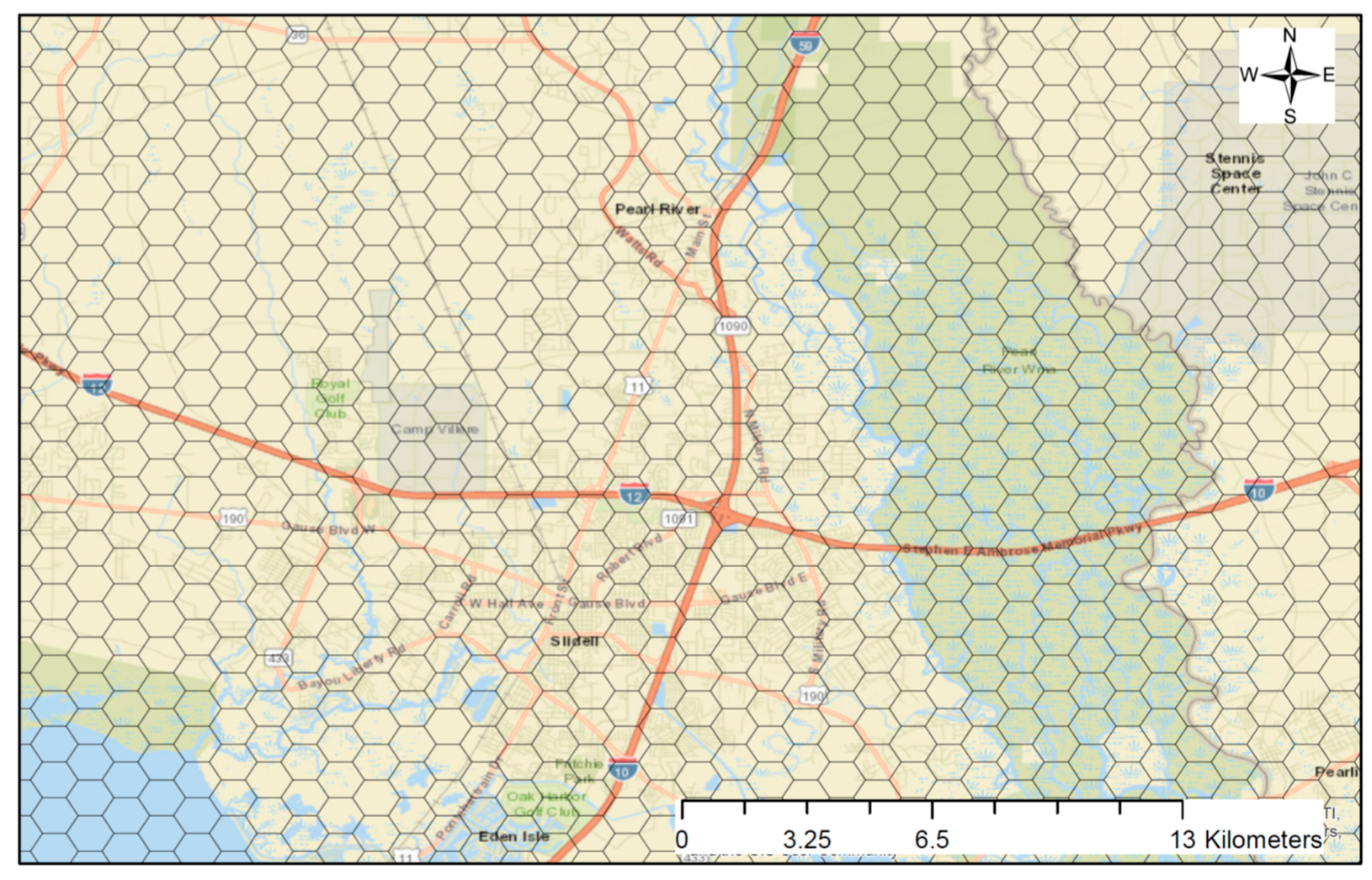
In this work, the SCA region (Figure 1) was partitioned into an equal area hexagonal grid (side length of 0.61 km and area of 1 km2 see Figure 2). Hexagonal grids are preferred over other geometrical shapes (e.g., square or triangle) because they are characterized by elements that do not have gaps or overlaps and the center-to-center distances between neighboring cells are almost equal [36]. Furthermore, hexagonal cells have a topology that is symmetric, invariant, and of equal area and can be recursively partitioned into smaller divisions of grids if or when required to represent higher resolution data types.
The geodatabase was included within the hexagonal grid as an Esri Shapefile that stored nontopological geometry and attribute information for the spatial features in the dataset. An ESRI shapefile consists of a main file (.shp), an index file (.shx), a dBASE table (.dbf), a projection file (.prj), and a metadata file (.xml) that is compliant with the Federal Geographic Data Committee [37]. These data can be read in commercial GIS tools such as ArcMap and open source programs such as QGIS, R, and Python. The Esri Shapefile can also be converted into other file formats such as GeoJSON using open source tools.

3.2. Data Processing Workflow

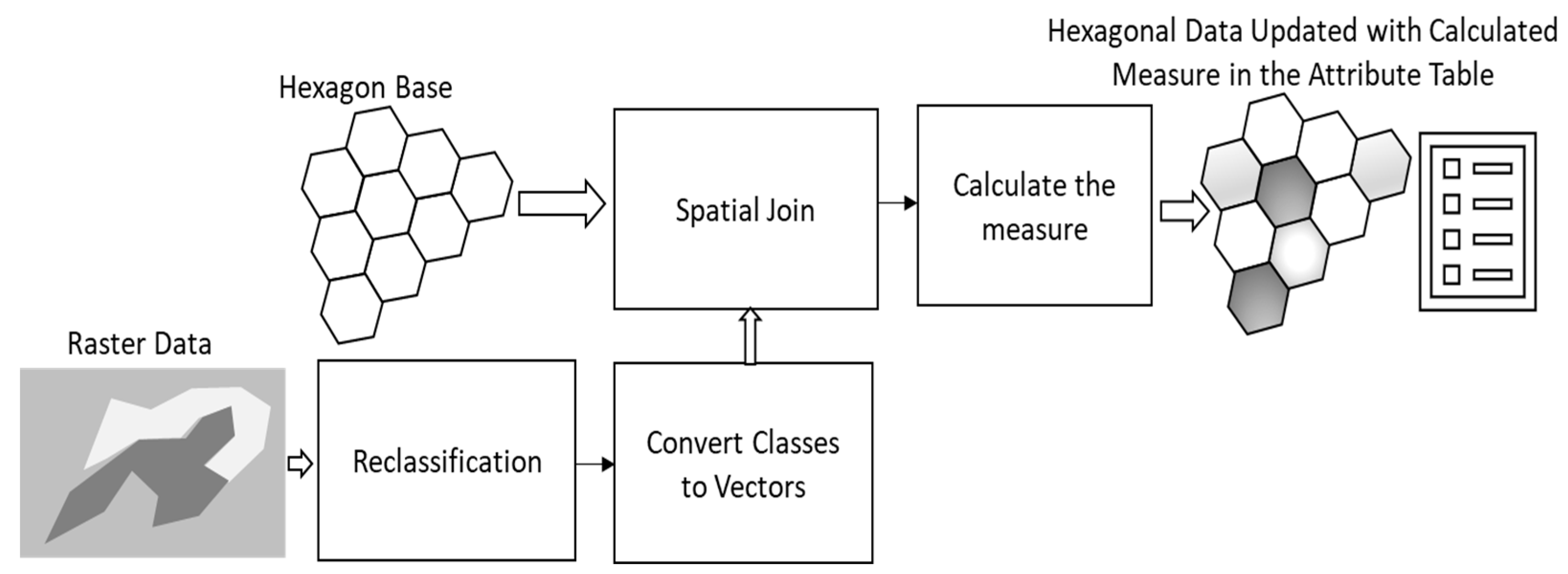
The methods used to process each measure were dependent on the type of source data (i.e., vector or raster) and the type of measure unit (i.e., index, binary, percentage area, count, or length). See Table 3 for a more detailed summary of the source data type and measure unit type for each of the 19 measures. Figure 3 and Figure 4 provide a visualization of the general workflow used to produce measures from vector and raster source data, respectively. Appendix A provides more detailed steps for how we produced each measure.

3.3. Data Overview

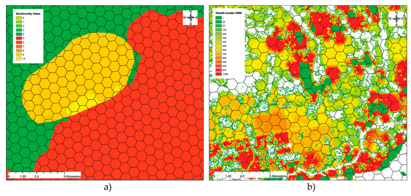
Figure 5a–e illustrate the five different types of data measures in preprocessed states (i.e., index, binary, percentage area, count, and length) that are present within the database. Figure 6a,b illustrate the two types of source data (i.e., vector and raster) that were utilized in processing the database measures.

4. User Notes

There are two potential sources of uncertainty that need to be considered with the use of this database. First is the time lag between source data production and when the database was created, which will depend on each measure. As time progresses, the accuracy of each measure will inevitably decline, but the database used the most recent version of each source datum to minimize any error induced by time lag. A second potential source of uncertainty came from the 1 km2. resolution that was used for the hexagonal grid. Since the measures were defined to describe general features of an area for conservation considerations and most lands conserved in this region were roughly 1 km2, the data resolution was adequate for assessments of the land conservation value. Caution should thus be noted if using this database for purposes other than the land conservation value.
The geodatabase is available at Scholar’s Junction, an institutional repository for Mississippi State University as a shapefile. A readme file is available for download along with the database where the user can find instructions for how to convert the database from GeoJSON to other formats. The codebase of the SCA project is available through github and the details of the project can be found at Landscope webpage both provided as Supplementary Materials.

Supplementary Materials

Additional information about the Strategic Conservation Assessment of Gulf Coast Landscapes project for which this database was developed can be found at https://github.com/scatools and http://www.landscope.org/gulfcoast.

Author Contributions

S.S. conceived of the idea of this paper. A.S. and S.S. performed the writing. J.L., A.S., and S.S. led the data processing. J.R. led the stakeholder charrettes and provided rankings of priority attributes. K.E., J.R., and A.L. initiated discussions with experts on refining and using the data sources. K.E. and A.L. contributed to writing and revisions. All authors have read and agreed to the published version of the manuscript.

Funding

This research was funded by the United States Department of Interior, Grant Number F17AC00267.

Acknowledgments

This paper is a contribution of the Mississippi Agricultural and Forestry Experiment Station and the Forest and Wildlife Research Center, Mississippi State University, with funding support from a Gulf Coast Ecosystems Studies Unit cooperative agreement with the U.S. Fish and Wildlife Service and under support from the Gulf Coast Ecosystem Restoration Council. The authors would like to thank John Tirpak, Rachel Kirpes, Ben Wilson, Chris Pease, Matt Snider, David Reeves, and Stephanie Sharuga from U.S. Fish and Wildlife Service; Steve Ashby and Wes Burger from Mississippi State University; and Jessica Henkel from the Gulf Ecosystem Restoration Council for their contributions to this work. Additional thanks are extended to Randy Clark from the National Oceanic and Atmospheric Administration, Mark Defley from the U.S. Department of Agriculture, Rua Mordecai from the South Atlantic Landscape Conservation Cooperative (LCC), Todd Jones-Farrand from the U.S. Fish and Wildlife Service, Tom Strange from the Mississippi Department of Environmental Quality, Will Underwood from the Alabama Department of Conservation and Natural Resources, Beth Stys from the Florida Fish and Wildlife Conservation Commission, Laura Chapa from the Texas Parks and Wildlife Department, and Jon Oetting from the Florida Natural Areas Inventory for their valuable inputs on data sources and usage.

Conflicts of Interest

The authors declare no conflicts of interest.

Appendix A. Definition and Implementation of Database Measures

Appendix A.1. Threat of Urbanization

Definition: Threat of urbanization (ToU) indicates the likelihood of the given project area or area of interest (AOI) being urbanized by the year 2060. A ToU score of zero indicates the AOI is already urbanized. A ToU score of one indicates that there is absolutely no threat of urbanization. A ToU score between zero and one indicates the predicted likelihood of threat in decreasing order. Source data came from the SLEUTH model [3,4,5,6].
Workflow:
  • Reclassify raster values from 0–1000 in 16 classes (1 to 1000), where Ai represents the area of the ith class within a hexagon).
  • Convert individual classes to vectors.
  • Crop the vector classes to hexagon boundaries, and perform spatial joins to obtain areas of each vector class within hexagons.
  • ToU is then calculated as shown in Equation (A1).
ToU   =   1     ( 0.025 A 25   +   0.05 A 50   +   0.1 A 100 +   0.2 A 200 +   0.3 A 300 +   0.4 A 400   +   0.5 A 500 +   0.6 A 600 +   0.7 A 700 +   0.8 A 800 +   0.9 A 900 +   0.95 A 950   +   0.975 A 975   + 1.0 A 1000 + 1 A 1 )

Appendix A.2. Connectivity to Existing Protected Area

Definition: Connectivity to existing protected area indicates if the proposed conservation area is close to an area classified as protected by Protected Areas Database of the United States (PAD-US) 2.0 data [7]. Protected areas included International Union for Conservation of Nature (IUCN) Categories Ia-VI and U.S. Geological Survey Gap Analysis Program (GAP) Status 1–4 areas. A binary attribute represents the spatial relationship between a hexagon and a protected area within PAD-US 2.0. Any hexagon that directly intersects or is within a 1 km distance of a protected area would count as one, otherwise, zero.
Workflow:
  • Create a 1 km buffer around PAD-US 2.0 data.
  • Perform spatial overlay of the PAD-US 2.0 buffer with hexagon boundaries
  • Classify the hexagons as connected (one) or not connected (zero) based on the overlap between a hexagon and the buffer

Appendix A.3. Structural Connectivity

Definition: A percent attribute that stands for the proportion of area classified as a hub or corridor, according to the Intact Habitat Cores layer from Esri’s Green Infrastructure Initiative [8]. This attribute prioritizes large protected areas and critical corridor connections.
Workflow:
  • Convert the Intact Habitat Cores layer to vector format.
  • Merge Hub and Connectivity layers.
  • Perform spatial join with hexagon boundaries to extract areas.

Appendix A.4. Composition of Natural Lands

Definition: This attribute prioritizes rare habitat types and those that have been identified as conservation priorities in state and regional plans. Scores reflect the proportion (%) of each area of interest that is covered by a priority land cover. Source data came from USGS GAP (2011) [9], Florida Cooperative Land Cover 3.3 by the Florida Fish & Wildlife Conservation Commission (FWC) [10], and Texas Ecological Mapping Systems (TX EMS) by the Texas Parks & Wildlife Department (TPWD) [11].
Workflow:
  • Mosaic TX, FL, and GAP data together.
  • Compile appropriate classes within assigned categories.
  • Resample TX to 30 m resolution.
  • Rank classifications of landcover within the hexagons (see Table A1).
Table A1. Categorization (tier) of landcover classes for ranking in the composition of natural lands.
Tier 1State Wildlife Action Plan (SWAP) Tier 1 habitats
Gulf Coast Vulnerability Assessment ecosystems:
mangrove
tidal emergent marsh
oyster reef
barrier islands
LCC priority habitats: GCP LCC, GCPO LCC, PF LCC
Other prioritized natural lands not overlapping with Tier 1
Tier 2managed pine
rangelands
hay
crop lands
low density residential
Tier 3urban
commercial
barren
open water

Appendix A.5. 303(d): Impaired Watershed Area

Definition: A percent attribute that stands for the proportion of impaired watershed within each hexagon. The watershed data are analyzed based on the 12-digit hydrologic unit code (HUC-12) level. Any HUC-12 watershed that contains an Environmental Protection Agency (EPA) 303(d) listed impaired waterbody would be considered impaired [12].
Workflow:
  • Clip the impaired watershed boundary layer with hexagon boundaries.
  • Perform spatial join to calculate the proportion of each hexagon that contains an impaired watershed.

Appendix A.6. Hydrologic Response to Land Use Change

Definition: A percent attribute that stands for the change in peak flow during a 24 h 1 rainfall event of an HUC-12 watershed at its currently developed state relative to its hypothetical pre-developed state. The pre-developed state was created by replacing all anthropogenic land cover with the most dominant natural land cover found within the HUC-12 watershed. All land cover used in this measure came from the National Land Cover Database (NLCD) 2016 [14].
Workflow:
  • Perform spatial join of the vector data with hexagon boundaries.
  • Compute mean of percent change in peak flow values within each hexagon.

Appendix A.7. Stream Abundance

Definition: A numerical attribute that quantifies the length of streams (km) found within a hexagon. Stream data came from the National Hydrography Dataset Plus Version 2 (NHDPlusV2)-NHD Snapshot [13].
Workflow:
  • Clip the NHD Snapshot stream vectors to the hexagon boundaries.
  • Calculate the length of all streams within each hexagon.

Appendix A.8. Biodiversity Index

Definition: The biodiversity index is on a continuous zero-to-ten range representing prioritized species richness for more than 1200 endemic mammals, birds, amphibians, reptiles, freshwater fish, and trees in the U.S. An index of zero indicates the lowest under-protected (vulnerable) biodiversity. An index of 10 indicates the highest under-protected biodiversity. Source data came from the U.S. protected lands mismatch biodiversity priorities, by Jenkins et al. [16].
Workflow:
  • Classify the raster into 10 classes.
  • Vectorize 10 classes.
  • Perform spatial join with the hexagon boundaries.
  • Compute the mean of biodiversity values within each hexagon.

Appendix A.9. Threatened and Endangered Species Critical Habitat Area

Definition: The attribute is based on the U.S. Fish and Wildlife Service designated T&E critical habitat [17]. The value in each hexagon is the cumulative % area of critical habitats for all T&E species.
Workflow:
  • Exclude the species not found in the SCA region and the areas of critical habitat not contained in the SCA region.
  • For each species i, calculate the proportion of critical habitat for species in the SCA region contained within a hexagon (Asi) using Equation (A2).
  • Calculate T&E percent area using Equation (A3).
A S i =   Area   of   critical   habitat   for   species   i   that   intersects   with   the   hexagon Total   area   of   critical   habitat   for   species   i
T & E   P e r c a n t a g e   A r e a =   i A S i

Appendix A.10. T&E Species Counts

Definition: This attribute measures the number of threatened and endangered (T&E) species that have habitat ranges identified within each hexagon. The source data came from the U.S. Fish and Wildlife Service designated T&E habitat ranges [18].
Workflow:
  • Perform spatial join of the data with hexagon boundaries.
  • Obtain the counts within each hexagon.

Appendix A.11. Light Pollution Index

Definition: An index that measures the intensity of light pollution within each hexagon. A score of zero indicates that the sky above the hexagon is already polluted/bright, and a score of 0+ to 1 indicates light pollution (LP) in decreasing order. Source data came from Falchi et al. [19].
Workflow:
  • Reclassify raster values from 0–30 to zero (Z), low (L), medium (M), and high (H) as per the thresholds shown in Table A2 below.
  • Convert Z, L, M, and H classes to vectors.
  • Crop the vector classes to hexagon boundaries and perform spatial joints to obtain areas (AZ, AL, AM, and AH).
  • The LP index is then calculated as shown in Equation (A4).
Table A2. Description of discretized values used to calculate Light Pollution Index.
ClassLP Score
AZ0
AL1–10
AM11–20
AH21–30
L i g h t   P o l l u t i o n   I n d e x = 1 ( 0.33 A L + 0.66 A M + A H )

Appendix A.12. National Register of Historic Places

Definition: A numeric attribute that represents the counts of historic places within each hexagon. The data were based on the U.S. National Park Service’s National Register of Historic Places Program [20].
Workflow
  • Perform spatial join of the data with hexagon boundaries.
  • Obtain the counts within each hexagon.

Appendix A.13. National Heritage Area

Definition: A percent attribute that stands for the proportion of heritage area within each hexagon. The heritage data were based on the U.S. National Park Service’s National Heritage Area layer [21].
Workflow:
  • Clip the national heritage area data to hexagon boundaries.
  • Perform spatial join to obtain the area within each hexagon.

Appendix A.14. Proximity to Socially Vulnerable Communities

Definition: This measure indicates the proximity to communities that are socially vulnerable according to the National Oceanic and Atmospheric Administration’s (NOAA) Social Vulnerability Index. This is a binary attribute that represents the spatial relationship between a hexagon and areas that have been identified by NOAA as having medium or higher social vulnerability. Any area of interest that directly intersects or is within a 1 hex (1 km2) distance of a socially vulnerable community would score a one, and areas of interest not within a 1 km2 distance of a socially vulnerable community would score a zero. Source data came from the Social Vulnerability Index of Coastal Communities, from NOAA’s Office of Coastal Management [22,23].
Workflow:
  • Clip NOAA’s Social Vulnerability Index to hexagon boundaries.
  • Perform spatial join to obtain the Social Vulnerability Index within 1 km of each hexagon.

Appendix A.15. Community Threat Index

Definition: The Community Threat Index (CTI) comes from the Coastal Resilience Evaluation and Siting Tool (CREST), by the National Fish and Wildlife Foundation (NFWF) in collaboration with National Oceanic and Atmospheric Administration (NOAA), U.S. Army Corps of Engineers (USACE), and NatureServe [24] and includes datasets that show coastal flood and severe storm hazards on the landscape. The Threat Index is a raster based model (30 × 30 meters) with a cumulative scoring of inputs, which include: storm surge scenarios, sea level rise scenarios, flood prone areas, soil erodibility, impermeable soils, areas of low slope, and geologic stressors (i.e., landslide susceptibility and land subsidence).
Workflow:
  • Transform the CTI raster data to a vector shapefile.
  • Perform spatial join to obtain the CTI within each hexagon.

Appendix A.16. Working Lands: High Priority

Definition: The percentage area of pine, cropland and pasture/hay classes from the National Land Cover Database (NLCD) 2016 classification map [14] excluding the areas that are already protected according to the Protected Areas Database of the United States (PAD-US) 2.0 [7].
Workflow:
  • Extract the target layers from NLCD 2016 to a new raster file.
  • Transform the raster data to a vector shapefile.
  • Perform spatial join to calculate the percent area within each hexagon.

Appendix A.17. Commercial Fishing Reliance

Definition: Commercial fishing reliance measures the presence of commercial fishing through fishing activity as shown through permits and vessel landings relative to the population of a community. A high rank indicates more reliance. The data source for this measure came from the Social Indicators of Fishing Community Vulnerability and Resilience, by the National Marine Fisheries Service (NMFS) [25,26]. More information can be found at st.nmfs.noaa.gov/humandimensions/social-indicators/.
Workflow:
  • Clip the Commercial fishing reliance data to hexagon boundaries.
  • Perform spatial join to obtain the commercial fishing reliance data within each hexagon.

Appendix A.18. Recreational Fishing Engagement

Definition: Recreational fishing engagement measures the presence of recreational fishing through fishing activity estimates, including charter fishing pressure, private fishing pressure, and shore fishing pressure. A high rank indicates more engagement. The data source for this measure came from the Social Indicators of Fishing Community Vulnerability and Resilience, by the National Marine Fisheries Service (NMFS) [25,26]. More information can be found at st.nmfs.noaa.gov/humandimensions/social-indicators/.
Workflow:
  • Clip the recreational fishing engagement data to hexagon boundaries.
  • Perform spatial join to obtain the recreational fishing engagement data within each hexagon.

Appendix A.19. Access and Recreation: Number of Access Points

Definition: This measure indicates the number of points within a 25 km buffer radius of a hexagon, where the public can access places to engage in outdoor recreation, including boat ramps and access points to parks, wildlife management areas, wildlife refuges, and national estuarine research reserves. Besides boat ramps, access points to protected areas were identified by intersections between roadways and protected areas listed under the Protected Areas Database for the United States (PAD-US) 2.0 [7]. Roadways were acquired from the Topologically Integrated Geographic Encoding and Referencing (TIGER)/Line Shapefile by the United States Census Bureau (USCB) [32]. Public boat ramps were obtained from the Florida Fish & Wildlife Conservation Commission (FWC) [27], Alabama Dept. of Natural Resources (ALDNR) [28], Mississippi Dept. of Marine Resources (MDMR) [29], Louisiana Dept. of Wildlife & Fisheries (LDWF) [30], and Texas Parks & Wildlife Dept. (TPWD) [31].
Workflow:
  • Clip the access points data to hexagon boundaries.
  • Create a 25 km buffer around the centroid of each hexagon.
  • Obtain the counts of access points that intersect with the 25 km buffer of each hexagon.

References

  1. Samiappan, S.; Shamaskin, A.; Liu, J.; Roberts, J.; Linhoss, A.; Evans, K. Land Conservation in the Gulf of Mexico Region: A Comprehensive Review of Plans, Priorities, and Efforts. Land 2019, 8, 84. [Google Scholar] [CrossRef] [Green Version]
  2. Initial Comprehensive Plan: Restoring the Gulf Coast’s Ecosystem & Economy; Gulf Coast Ecosystem Restoration Council: New Orleans, LA, USA, 2013. Available online: https://www.restorethegulf.gov/sites/default/files/Final%20Initial%20Comprehensive%20Plan.pdf (accessed on 10 April 2018).
  3. Chaudhuri, G.; Clarke, K.C. The SLEUTH Land Use Change Model: A Review. Int. J. Environ. Resour. Res. 2013, 1, 89–104. [Google Scholar]
  4. Clarke, K.C. Project Gigalopolis-SLEUTH Urbanization Model; USGS and UCSB; Available online: http://www.ncgia.ucsb.edu/projects/gig/index.html (accessed on 12 July 2018).
  5. Clarke, K.C. Mapping and Modelling Land Use Change: An Application of the SLEUTH Model. In Landscape Analysis and Visualisation: Spatial Models for Natural Resource Management and Planning; Pettit, C., Cartwright, W., Bishop, I., Lowell, K., Pullar, D., Duncan, D., Eds.; Springer: Berlin, Germany, 2008; pp. 353–366. ISBN 978-3-540-69168-6. [Google Scholar]
  6. Terando, A.J.; Costanza, J.; Belyea, C.; Dunn, R.R.; McKerrow, A.; Collazo, J.A. The Southern Megalopolis: Using the Past to Predict the Future of Urban Sprawl in the Southeast, U.S. PLoS ONE 2014, 9, e102261. [Google Scholar] [CrossRef] [PubMed] [Green Version]
  7. Gergeley, K.J.; McKerrow, A. PAD-US—National Inventory of Protected Areas; USGS: Reston, VA, USA, 2016; p. 2.
  8. Perkl, R. Intact Habitat Cores Map. Available online: https://www.arcgis.com/home/item.html?id=b9155ee0caa04fcf9744e25cad76b44a (accessed on 12 October 2019).
  9. USGS. U.S. Geological Survey Gap Analysis Program; GAP/LANDFIRE National Terrestrial Ecosystems; USGS: Reston, VA, USA, 2011.
  10. Florida FWS-Cooperative Land Cover, Version 3.3; Florida Fish and Wildlife Conservation Commission: Tallahassee, FL, USA, 2019.
  11. TX-TPWD. Texas Ecological Mapping Systems-TXEMS; Texas Parks and Wildlife: Austin, TX, USA. Available online: https://tpwd.texas.gov/landwater/land/programs/landscape-ecology/ems/emst (accessed on 6 March 2019).
  12. Clean Water Act; EPA: Washington, DC, USA, 1972.
  13. McKay, L.; Bondelid, T.; Dewald, T.; Johnston, J.; Moore, R.; Reah, A. NHDPlus Version 2: User Guide 2012. Available online: https://nctc.fws.gov/courses/references/tutorials/geospatial/CSP7306/Readings/NHDPlusV2_User_Guide.pdf (accessed on 3 April 2019).
  14. Yang, L.; Jin, S.; Danielson, P.; Homer, C.; Gass, L.; Bender, S.M.; Case, A.; Costello, C.; Dewitz, J.; Fry, J.; et al. A new generation of the United States National Land Cover Database: Requirements, research priorities, design, and implementation strategies. ISPRS J. Photogramm. Remote. Sens. 2018, 146, 108–123. [Google Scholar] [CrossRef]
  15. Soil Survey Staff Web Soil Survey; Natural Resources Conservation Service; USDA: Washington, DC, USA, 2018.
  16. Jenkins, C.N.; Van Houtan, K.S.; Pimm, S.L.; Sexton, J.O. US protected lands mismatch biodiversity priorities. Proc. Natl. Acad. Sci. USA 2015, 112, 5081–5086. [Google Scholar] [CrossRef] [PubMed] [Green Version]
  17. U.S. Fish and Wildlife Service Environmental Conservation Online System Critical Habitat Report. Available online: https://ecos.fws.gov/ecp/report/table/critical-habitat.html (accessed on 17 July 2018).
  18. U.S. Fish and Wildlife Service Environmental Conservation Online System All Threatened and Endangered Species Range. Available online: https://ecos.fws.gov/ecp/ (accessed on 10 July 2018).
  19. Falchi, F.; Cinzano, P.; Duriscoe, D.; Kyba, C.C.M.; Elvidge, C.D.; Baugh, K.; Portnov, B.; Rybnikova, N.A.; Furgoni, R. Supplement to: The New World Atlas of Artificial Night Sky Brightness. GFZ data services (2016). Available online: http://dataservices.gfz-potsdam.de/panmetaworks/showshort.php?id=escidoc:1541893&contactform (accessed on 15 October 2018).
  20. Stutts, M. National Register of Historic Places. National Register Properties Are Located throughout the United States and Their Associated Territories around the Globe. Available online: https://irma.nps.gov/DataStore/Reference/Profile/2210280 (accessed on 7 July 2018).
  21. National Park Service. National Heritage Areas. Available online: https://www.nps.gov/subjects/heritageareas/index.htm (accessed on 7 July 2018).
  22. Emrich, C.T.; Cutter, S.L. Social Vulnerability to Climate-Sensitive Hazards in the Southern United States. J. Weather Clim. Soc. 2011, 3, 193–208. [Google Scholar] [CrossRef]
  23. University of South Carolina. NOAA Office for Coastal Management Social Vulnerability Index 2010 (Census Tracts); University of South Carolina Press: Columbia, SC, USA, 2010. [Google Scholar]
  24. National Fish and Wildlife Foundation; National Oceanic and Atmospheric Administration; U.S. Army Corps of Engineers; National Environmental Modeling and Analysis Center. NatureServe Coastal Resilience Evaluation and Siting Tool. Available online: https://resilientcoasts.org (accessed on 5 May 2019).
  25. Colburn, L.L.; Jepson, M.; Weng, C.; Seara, T.; Weiss, J.; Hare, J.A. Indicators of climate change and social vulnerability in fishing dependent communities along the Eastern and Gulf Coasts of the United States. Mar. Policy 2016, 74, 323–333. [Google Scholar] [CrossRef]
  26. Jepson, M.; Colburn, L.L. Development of Social Indicators of Fishing Community Vulnerability and Resilience in the U.S. Southeast and Northeast Regions. Available online: https://repository.library.noaa.gov/view/noaa/4438 (accessed on 3 June 2018).
  27. Florida Fish and Wildlife Conservation Commission. Florida Public Boat Ramp Finder. Available online: https://public.myfwc.com/LE/boatramp/public/Default.aspx (accessed on 23 August 2019).
  28. Alabama Department of Conservation and Natural Resources. Coastal Alabama Boating Access. Available online: https://www.outdooralabama.com/boating/coastal-alabama-boating-access (accessed on 21 September 2019).
  29. Mississippi Department of Marine Resources. Public Access Inventory. Available online: http://gis.dmr.ms.gov/PublicAccess/ (accessed on 10 August 2019).
  30. Louisiana Department of Wildlife and Fisheries. Louisiana Outdoor Explorer. Available online: http://ldwf.maps.arcgis.com/apps/MapSeries/index.html?appid=4c4a4d9526c248c080c3eaa4808b9bea (accessed on 19 June 2019).
  31. Texas Parks and Wildlife Department. Public Boat Ramps. Available online: http://www.landscope.org/texas/tx_map_layers/tx_recreation_layers/ramps_for_boats/24760/ (accessed on 10 August 2019).
  32. U.S. Department of Commerce, U.S. Census Bureau, Geography Division TIGER/Line Shapefile. Series Information for the All Lines County-based Shapefile. Available online: https://www.census.gov/geographies/mapping-files/time-series/geo/tiger-line-file.html (accessed on 15 August 2019).
  33. Esri ArcGIS Desktop; Environmental Systems Research Institute: Redlands, CA, USA, 2019.
  34. R Core Team. R: A Language and Environment for Statistical Computing; R Core Team: Vienna, Austria, 2019. [Google Scholar]
  35. Cheng, J.; Karambelkar, B.; Xie, Y. Leaflet: Create Interactive Web Maps with the Javascript “Leaflet” Library. Available online: https://rdrr.io/cran/leaflet/ (accessed on 20 December 2019).
  36. Goldblatt, R.; Stuhlmacher, M.F.; Tellman, B.; Clinton, N.; Hanson, G.; Georgescu, M.; Wang, C.; Serrano-Candela, F.; Khandelwal, A.K.; Cheng, W.-H.; et al. Using Landsat and nighttime lights for supervised pixel-based image classification of urban land cover. Remote Sens. Environ. 2018, 205, 253–275. [Google Scholar] [CrossRef]
  37. FGDC Federal Geographic Data Committee. Content Standard for Digital Geospatial Metadata (FGDC CSDGM) FGDC-STD-001-1998; FGDC Federal Geographic Data Committee: Washington, DC, USA, 1998.
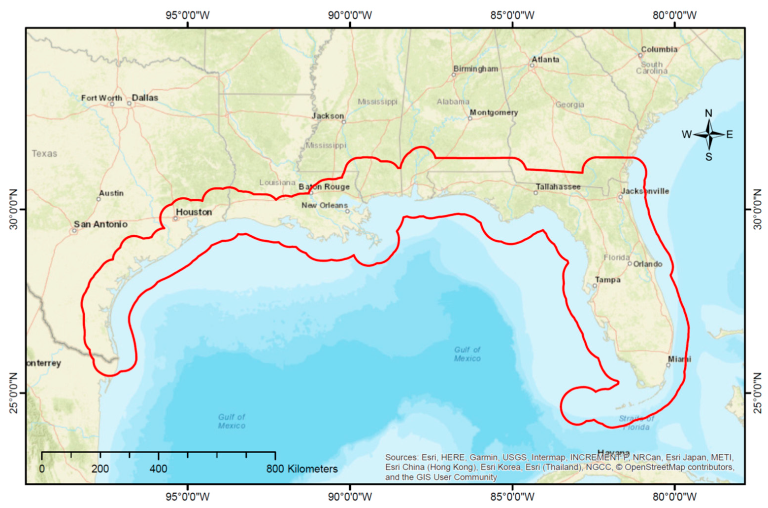
Figure 1. Overview of the Gulf of Mexico Coastal Region (GCR) along the U.S. Gulf of Mexico. The GCR includes the coastal management zone area of all the Gulf Coast states (i.e., Texas, Louisiana, Mississippi, Alabama, and Florida), plus 40.2 km inland of the coast including the barrier islands, as shown in the red outline.
Data 05 00003 g001
Figure 2. Snapshot of the 1 km2 hexagonal grid overlaid on a base map showing parts of coastal Mississippi and Louisiana.
Data 05 00003 g002
Figure 3. Visual aid of the steps involved to convert vector source data into a measure.
Data 05 00003 g003
Figure 4. Visual aid of the steps involved to convert raster source data into a measure.
Data 05 00003 g004
Figure 5. Measure types included within the geospatial database. (a) An example of an index measure using recreational fishing engagement. (b) An example of a binary measure using connectivity to existing protected area. (c) An example of a percentage area measure using 303(d) impaired watershed area. (d) An example of a count measure using the National Register of Historic Places. (e) An example of a length measure using stream abundance.
Data 05 00003 g005
Figure 6. Source data types: (a) An example of vector data using the biodiversity index [16]. (b) An example of raster data using the SLEUTH model [3,4,5,6].
Data 05 00003 g006
Table 1. Goals identified in the Gulf Coast Restoration Council [2]. RESTORE, Resources and Ecosystems Sustainability, Tourist Opportunities and Revived Economies of the Gulf Coast States.
RESTORE Goal 1Definition
1Restore and Conserve Habitat (HAB)Restore and conserve the health, diversity, and resilience of key coastal, estuarine, and marine habitats.
2Restore Water Quality and Quantity (WAQ)Restore and protect the water quality of the Gulf Coast region’s fresh, estuarine, and marine waters.
3Replenish and Protect Living Coastal and Marine Resources (LCMR)Restore and protect healthy, diverse, and sustainable living coastal and marine resources.
4Enhance Community Resilience (CRES)Build upon and sustain communities with capacity to adapt to short and long term changes.
5Restore and Revitalize the Gulf Economy (GEC)Enhance the sustainability and resiliency of the Gulf economy.
1 In the remainder of the manuscript, RESTORE goals will be referenced by the defined acronyms.
Table 2. Description of each measure, organized by the RESTORE goal that is available for use in the geodatabase.
RESTORE GoalMeasure 1UnitData Sources 2
1HABThreat of UrbanizationIndexSLEUTH (Slope, Land use, Exclusion, Urban extent, Transportation and Hillshade) cellular automaton model 3.0 beta [3,4,5,6]
2HABConnectivity to Existing Protected AreaIndexPAD-US 2.0 [7]
3HABStructural ConnectivityPercentageEsriIntact Habitat Cores [8]
4HABComposition of Natural LandsPercentageGap Analysis Program (GAP) [9]; Florida Cooperative Land Cover (FL CLC) [10]; Texas Ecological Mapping Systems (TX EMS) [11]
5WAQ303D: Impaired Watershed AreaPercentageEPA 303(d) list [12];
NHDPlusV2 [13]
6WAQHydrologic Response to Land Use ChangePercentageNLCD 2016 [14]; SSURGO [15]; NHDPlusV2 [13]
7WAQStream AbundanceKilometerNHDPlusV2 [13]
8LCMRBiodiversity IndexIndexU.S. protected lands mismatch biodiversity priorities [16]
9LCMRT&E Species AreaPercentageUSFWS Threatened and Endangered Species [17]
10LCMRT&E Species CountsCountUSFWS Threatened and Endangered Species [18]
11LCMRLight Pollution IndexIndexThe New World Atlas of Artificial Night Sky Brightness [19]
12CRESNational Registry of Historic PlacesCountNPS National Register of Historic Places [20]
13CRESNational Heritage AreaPercentageNPS National Heritage Area [21]
14CRESProximity to Socially Vulnerable CommunitiesBinaryNOAA Social Vulnerability Index [22,23]
15CRESCommunity Threat IndexIndexNFWF Coastal Resilience Evaluation and Siting Tool [24]
16GECWorking Lands: High PriorityPercentageGAP [9]; Florida Cooperative Land Cover (FL CLC) [10]; Texas Ecological Mapping Systems (TX EMS) [11]
17GECCommercial Fishing RelianceIndexNMFS Social Indicators [25,26]
18GECRecreational Fishing EngagementIndexNMFS Social Indicators [25,26]
19GECAccess and Recreation: Number of Access PointsCountFlorida Fish & Wildlife Conservation Commission [27]; Alabama Dept. of Conservation & Natural Resources [28]; Mississippi Dept. of Marine Resources [29]; Louisiana Dept. of Wildlife & Fisheries [30]; Texas Parks and Wildlife Dept. [31]; PAD-US 2.0 [7]; TIGER/Lines 2019 [32]
1 Refer to the Appendix A for the definitions of each measure, as well as the steps followed to represent them in a hexagonal grid. 2 Acronyms from the table are defined: SLEUTH, Slope, Land use, Exclusion, Urban extent, Transportation and Hillshade; PAD-US, Protected Areas Database of the United States; Esri, Environmental Systems Research Institute; EPA, Environmental Protection Agency; NHDPlusV2, National Hydrography Dataset Plus Version 2; NLCD, National Land Cover Database; SSURGO, Soil Survey Geographic Database; USFWS, U.S. Fish and Wildlife Service; T&E, threatened and endangered; NOAA, National Oceanic and Atmospheric Administration; NFWF, National Fish and Wildlife Foundation; NMFS, National Marine Fisheries Service; TIGER, Topologically Integrated Geograph Encoding and Referencing.
Table 3. Summary of source data type and measure unit type for each measure.
Source Data TypeMeasure TypeMeasure
Vector to MeasureIndex (0–1)Commercial fishing reliance
Recreational fishing engagement
Binary (0/1)Connectivity to existing protected area
Proximity to socially vulnerable communities
Percentage Area (%)303(d) impaired watershed area
Hydrologic response to land use change
T&E species area
National heritage area
Count (#)T&E species count
National register of historic places
Access and recreation
Length (km)Stream abundance
Raster to MeasureIndex (0–1)Threat of urbanization
Biodiversity index
Light pollution index
Community threat index
Percentage Area (%)Structural connectivity
Composition of natural lands
High priority working lands