A Trillion Coral Reef Colors: Deeply Annotated Underwater Hyperspectral Images for Automated Classification and Habitat Mapping


Abstract
1. Summary
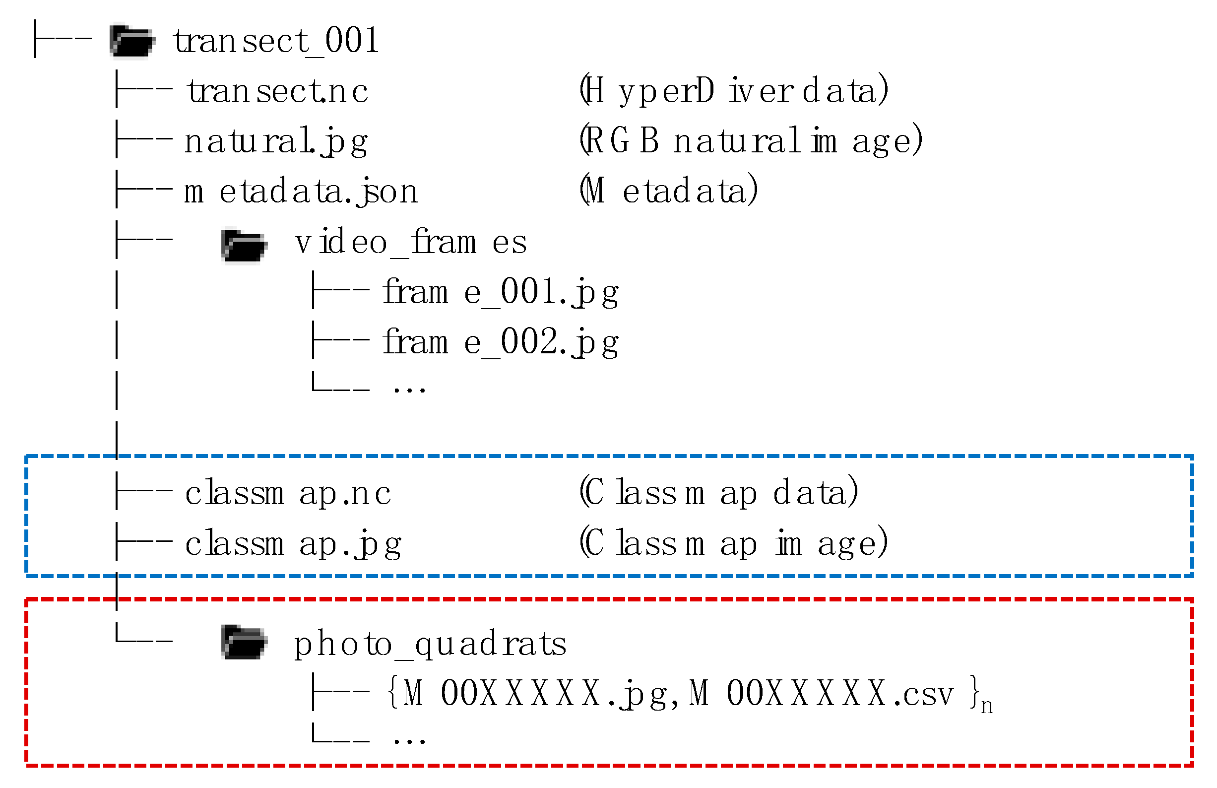
2. Data Description
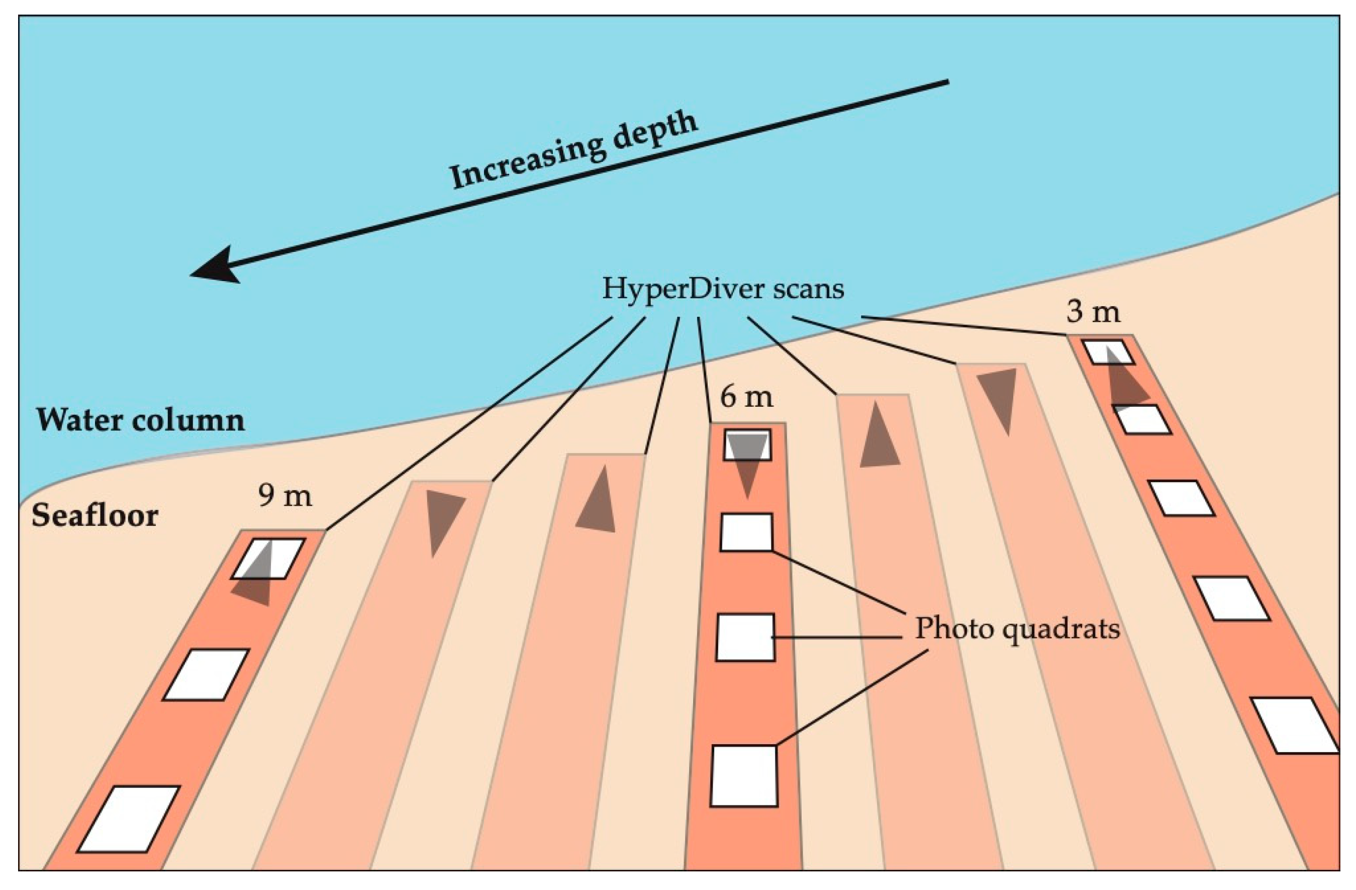
2.1. Photo Quadrat Survey Data
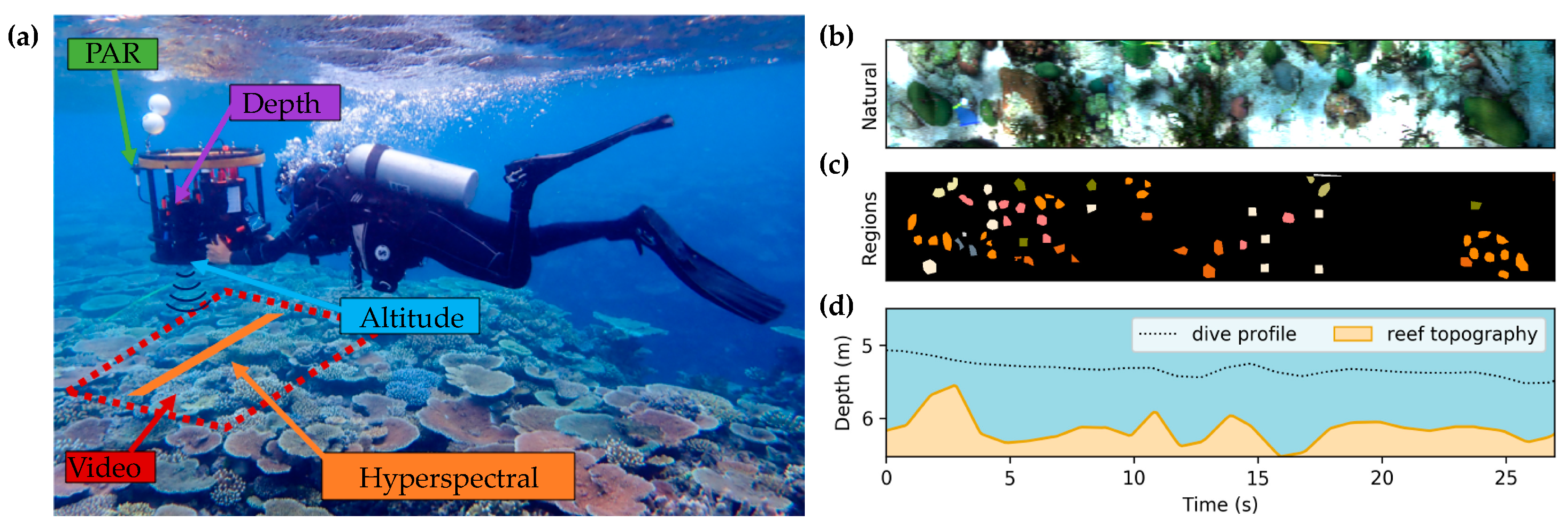
2.2. Hyper Diver Survey Data
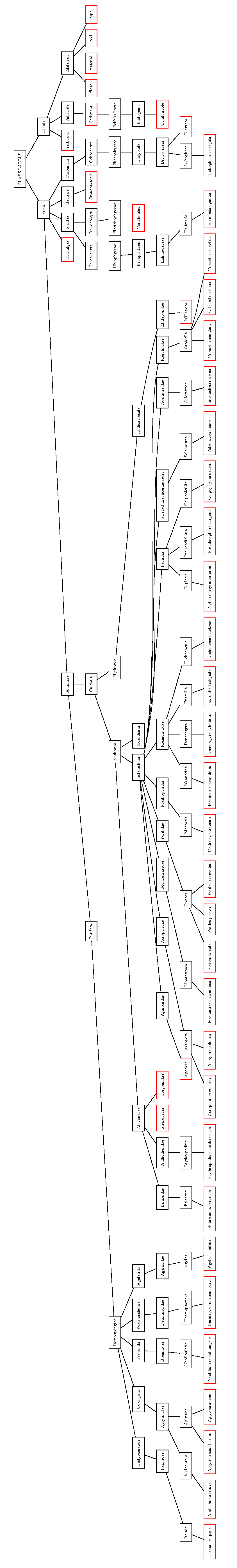
2.3. Benthic Habitat Description
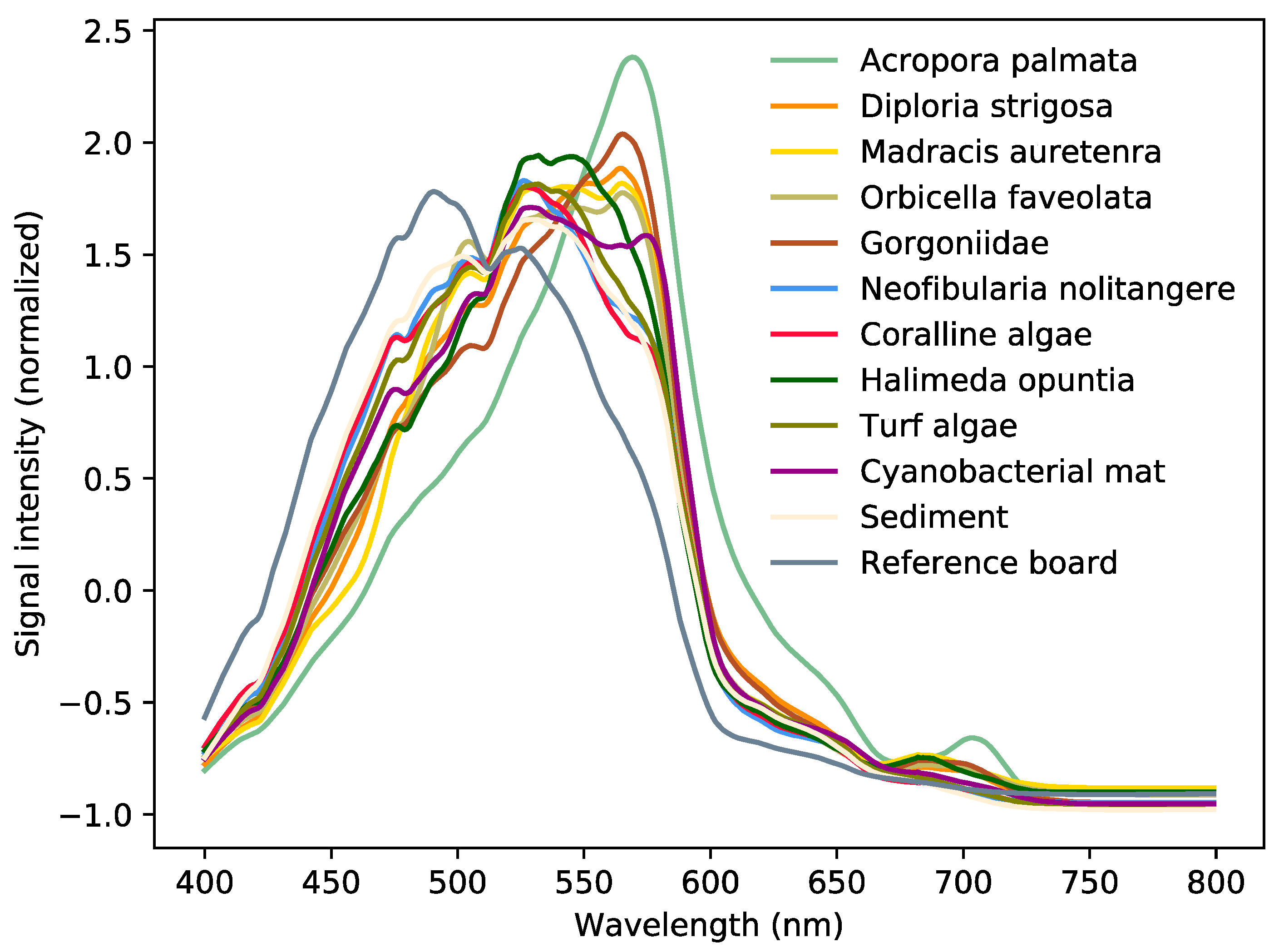
2.3.1. Targets for Image Segmentation
3. Methods
3.1. Data Acquisition
3.2. Hyper Diver Data Processing
3.3. Biodiversity and Substrate Labels for Habitat Mapping
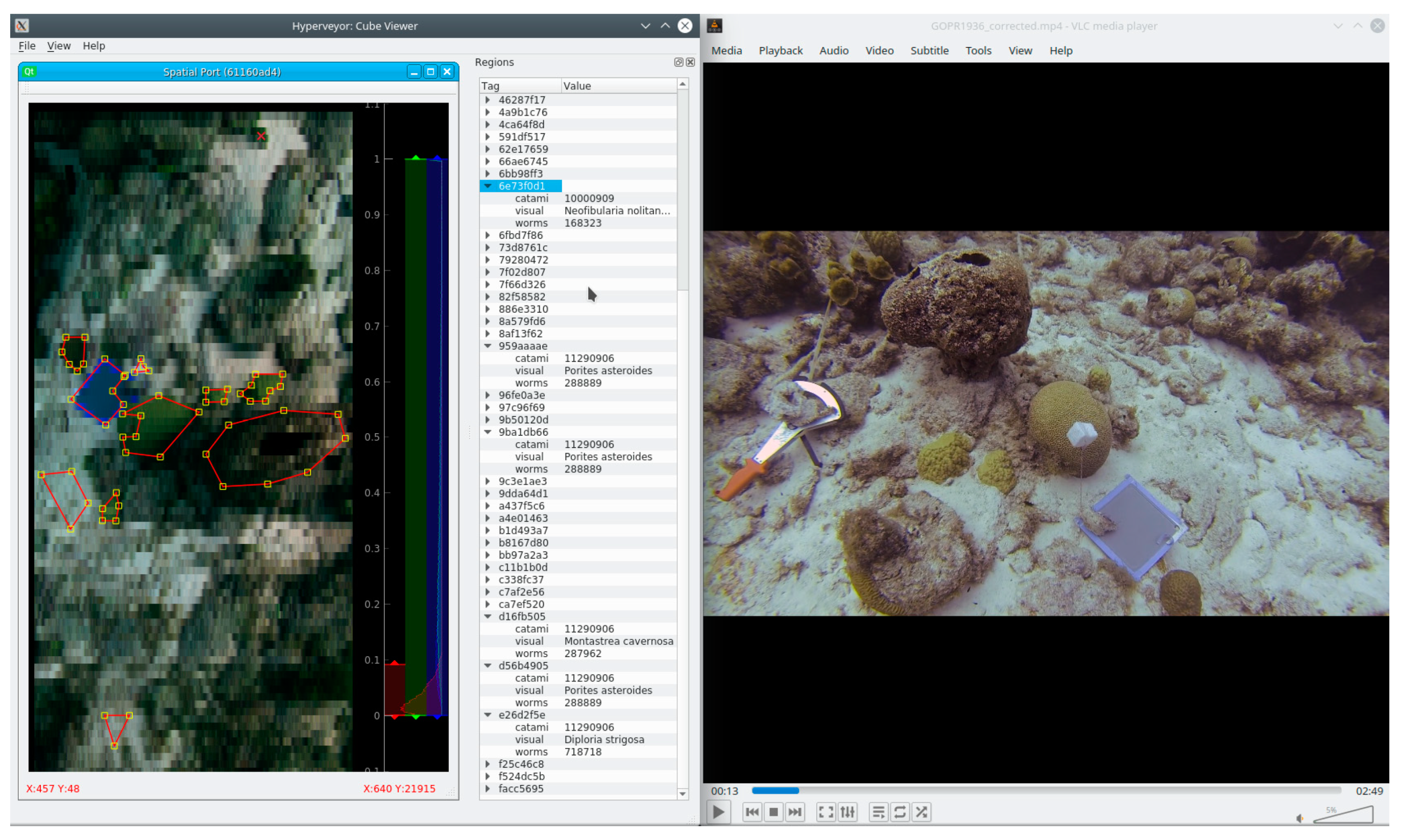
3.3.1. Annotation Strategy: Random Point Count Method
3.3.2. Annotation Strategy: Deliberate Bias to Reduce Human Effort
4. User Notes
Author Contributions
Funding
Acknowledgments
Conflicts of Interest
Appendix A

References
- Spalding, M.D.; Ravilious, C.; Green, E.P. World Atlas of Coral Reefs; University of California Press: Berkeley, CA, USA, 2001; ISBN 978-0-520-23255-6. [Google Scholar]
- Alcolado, P.M.; Alleng, G.; Bonair, K.; Bone, D.; Buchan, K.; Bush, P.G.; De Meyer, K.; Garcia, J.R.; Garzón-Ferreira, J.; Gayle, P.M.H.; et al. The Caribbean Coastal Marine Productivity Program (CARICOMP). Bull. Mar. Sci. 2001, 69, 819–829. [Google Scholar]
- Hodgson, G. Reef Check: The first step in community-based management. Bull. Mar. Sci. 2001, 69, 861–868. [Google Scholar]
- Roelfsema, C.M.; Phinn, S.R. Validation. In Coral Reef Remote Sensing; Goodman, J.A., Purkis, S.J., Phinn, S.R., Eds.; Springer: Dordrecht, The Netherlands, 2013; pp. 375–401. ISBN 978-90-481-9291-5. [Google Scholar]
- Maxwell, S.M.; Hazen, E.L.; Lewison, R.L.; Dunn, D.C.; Bailey, H.; Bograd, S.J.; Briscoe, D.K.; Fossette, S.; Hobday, A.J.; Bennett, M.; et al. Dynamic ocean management: Defining and conceptualizing real-time management of the ocean. Mar. Policy 2015, 58, 42–50. [Google Scholar] [CrossRef]
- Caras, T.; Hedley, J.; Karnieli, A. Implications of sensor design for coral reef detection: Upscaling ground hyperspectral imagery in spatial and spectral scales. Int. J. Appl. Earth Obs. Geoinf. 2017, 63, 68–77. [Google Scholar] [CrossRef]
- Chennu, A.; Färber, P.; De’ath, G.; de Beer, D.; Fabricius, K.E. A diver-operated hyperspectral imaging and topographic surveying system for automated mapping of benthic habitats. Sci. Rep. 2017, 7, 7122. [Google Scholar] [CrossRef] [PubMed]
- Dale, L.M.; Thewis, A.; Boudry, C.; Rotar, I.; Dardenne, P.; Baeten, V.; Pierna, J.A.F. Hyperspectral Imaging Applications in Agriculture and Agro-Food Product Quality and Safety Control: A Review. Appl. Spectrosc. Rev. 2013, 48, 142–159. [Google Scholar] [CrossRef]
- Ghiyamat, A.; Shafri, H.Z.M. A review on hyperspectral remote sensing for homogeneous and heterogeneous forest biodiversity assessment. Int. J. Remote Sens. 2010, 31, 1837–1856. [Google Scholar] [CrossRef]
- Wentz, E.; Anderson, S.; Fragkias, M.; Netzband, M.; Mesev, V.; Myint, S.; Quattrochi, D.; Rahman, A.; Seto, K. Supporting Global Environmental Change Research: A Review of Trends and Knowledge Gaps in Urban Remote Sensing. Remote Sens. 2014, 6, 3879–3905. [Google Scholar] [CrossRef]
- Wang, K.; Franklin, S.E.; Guo, X.; Cattet, M. Remote Sensing of Ecology, Biodiversity and Conservation: A Review from the Perspective of Remote Sensing Specialists. Sensors 2010, 10, 9647–9667. [Google Scholar] [CrossRef] [PubMed]
- Chang, C.-I. Hyperspectral Imaging: Techniques for Spectral Detection and Classification; Kluwer Academic/Plenum Publishers: New York, NY, USA, 2003; ISBN 978-0-306-47483-5. [Google Scholar]
- Mumby, P.J.; Green, E.P.; Edwards, A.J.; Clark, C.D. Coral reef habitat mapping: How much detail can remote sensing provide? Mar. Biol. 1997, 130, 193–202. [Google Scholar] [CrossRef]
- Pearlman, J.S.; Barry, P.S.; Segal, C.C.; Shepanski, J.; Beiso, D.; Carman, S.L. Hyperion, a space-based imaging spectrometer. IEEE Trans. Geosci. Remote Sens. 2003, 41, 1160–1173. [Google Scholar] [CrossRef]
- Asner, G.P.; Knapp, D.E.; Boardman, J.; Green, R.O.; Kennedy-Bowdoin, T.; Eastwood, M.; Martin, R.E.; Anderson, C.; Field, C.B. Carnegie Airborne Observatory-2: Increasing science data dimensionality via high-fidelity multi-sensor fusion. Remote Sens. Environ. 2012, 124, 454–465. [Google Scholar] [CrossRef]
- Foo, S.A.; Asner, G.P. Scaling Up Coral Reef Restoration Using Remote Sensing Technology. Front. Mar. Sci. 2019, 6, 79. [Google Scholar] [CrossRef]
- Gewali, U.B.; Monteiro, S.T.; Saber, E. Machine learning based hyperspectral image analysis: A survey. arXiv 2018, arXiv:1802.08701. [Google Scholar]
- Tasar, O.; Tarabalka, Y.; Alliez, P. Incremental Learning for Semantic Segmentation of Large-Scale Remote Sensing Data. IEEE J. Sel. Top. Appl. Earth Obs. Remote Sens. 2019, 12, 3524–3537. [Google Scholar] [CrossRef]
- Greenstein, B.J.; Pandolfi, J.M. Escaping the heat: Range shifts of reef coral taxa in coastal Western Australia. Glob. Chang. Biol. 2008, 14, 513–528. [Google Scholar] [CrossRef]
- Precht, W.F.; Aronson, R.B. Climate flickers and range shifts of reef corals. Front. Ecol. Environ. 2004, 2, 307–314. [Google Scholar] [CrossRef]
- WoRMS Editorial Board World Register of Marine Species. Available online: https://www.marinespecies.org (accessed on 4 December 2019). [CrossRef]
- Vandepitte, L.; Vanhoorne, B.; Decock, W.; Dekeyzer, S.; Trias Verbeeck, A.; Bovit, L.; Hernandez, F.; Mees, J. How Aphia—The Platform behind Several Online and Taxonomically Oriented Databases—Can Serve Both the Taxonomic Community and the Field of Biodiversity Informatics. J. Mar. Sci. Eng. 2015, 3, 1448–1473. [Google Scholar] [CrossRef]
- CATAMI Technical Working Group. CATAMI Classification Scheme for Scoring Marine Biota and Sub-Strata in Underwater Imagery. Version 1.4; National Environmental Research Program, Marine Biodiversity Hub: Canberra Australia, 2014. [Google Scholar]
- Pante, E.; Dustan, P. Getting to the Point: Accuracy of Point Count in Monitoring Ecosystem Change. J. Mar. Biol. 2012, 2012, 1–7. [Google Scholar] [CrossRef]
- Kohler, K.E.; Gill, S.M. Coral Point Count with Excel extensions (CPCe): A Visual Basic program for the determination of coral and substrate coverage using random point count methodology. Comput. Geosci. 2006, 32, 1259–1269. [Google Scholar] [CrossRef]


| Site Name | Site Location | Total Transects | Annotated Transects | Annotated ROIs | Annotated Pixels |
|---|---|---|---|---|---|
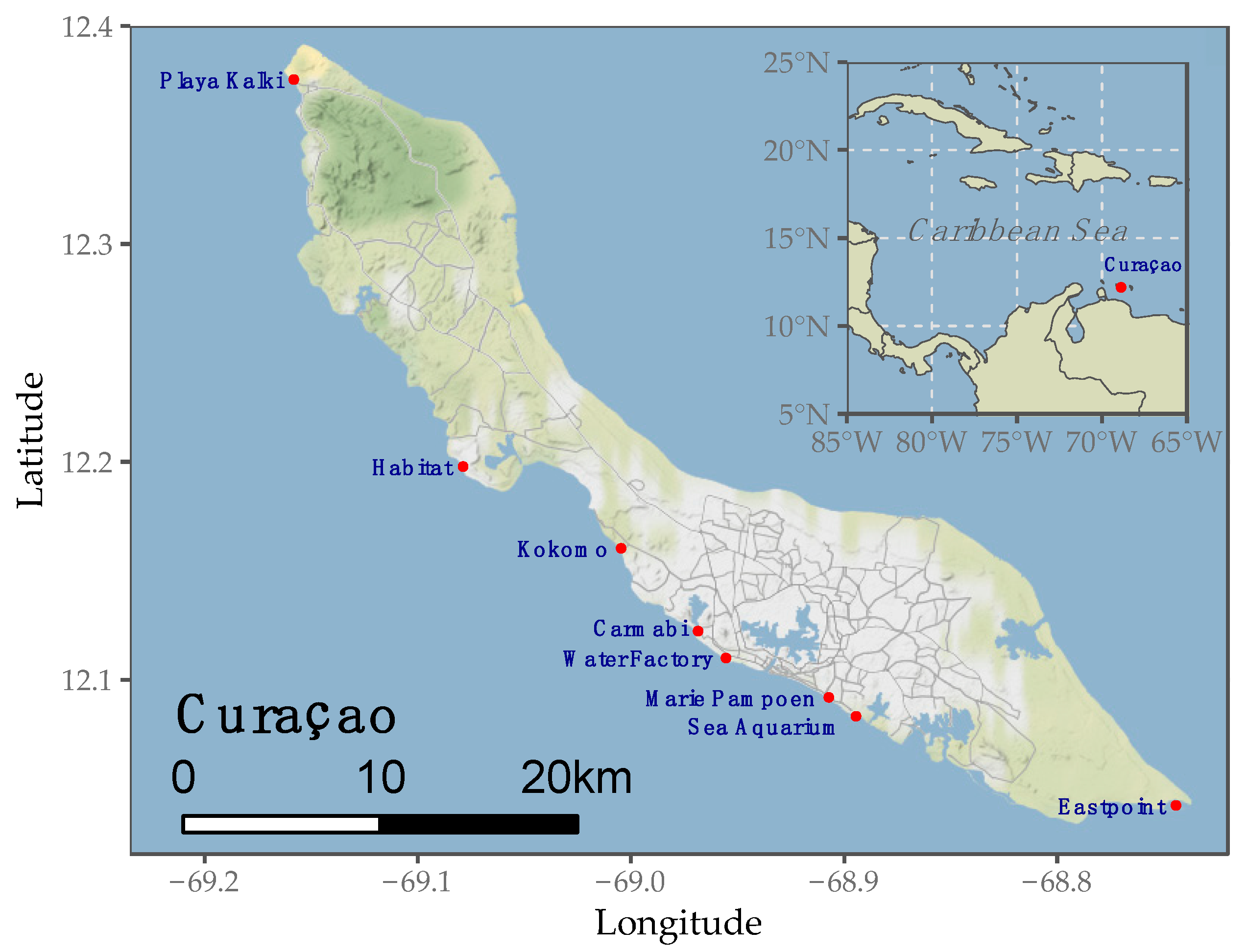
| Carmabi | 12.122331°N, 68.969234°W | 22 | 3 | 331 | 828,968 |
| Kokomo | 12.160331°N, 69.005403°W | 20 | 3 | 244 | 968,617 |
| Playa Kalki | 12.375344°N, 69.158931°W | 20 | 3 | 183 | 828,019 |
| Habitat | 12.197850°N, 69.079558°W | 22 | 3 | 231 | 775,872 |
| Water Factory | 12.109989°N, 68.956258°W | 10 | 3 | 377 | 1,347,646 |
| Marie Pampoen | 12.091894°N, 68.907918°W | 18 | 3 | 281 | 1,076,596 |
| Sea Aquarium | 12.083234°N, 68.895114°W | 15 | 2 | 117 | 1,117,412 |
| East Point | 12.042249°N, 68.745104°W | 20 | 3 | 325 | 1,264,642 |
| Total | 147 | 23 | 2089 | 8,207,772 |
| Category | Sub-Category/Morphology | Target Class | Annotated Regions |
|---|---|---|---|
| Coral | Branching | Acropora cervicornis | 2 |
| Acropora palmata | 1 | ||
| Madracis aurentenra | 3 | ||
| Coral | Massive/sub-massive | Diploria strigosa (Pseudodiploria strigosa) | 3 |
| Montastrea cavernosa | 3 | ||
| Orbicella faveolata | 3 | ||
| Orbicella annularis | 4 | ||
| Siderastrea siderea | 3 | ||
| Hydrozoan | Millepora sp. | 3 | |
| Macroalgae | Brown | Dictyota sp. | 4 |
| Macroalgae | Green | Halimeda opuntia | 3 |
| Soft coral | Gorgoniidae | 3 | |
| Plexauridae | 4 | ||
| Sponge | Barrel | Neofibularia nolitangere | 4 |
| Ircinia campana | 4 | ||
| Sponge | Massive | Aiolochroia crassa | 3 |
| Substrate | Sediment | 3 | |
| Coral rubble | 3 | ||
| Total | 56 |
© 2020 by the authors. Licensee MDPI, Basel, Switzerland. This article is an open access article distributed under the terms and conditions of the Creative Commons Attribution (CC BY) license (http://creativecommons.org/licenses/by/4.0/).
Share and Cite
Rashid, A.R.; Chennu, A. A Trillion Coral Reef Colors: Deeply Annotated Underwater Hyperspectral Images for Automated Classification and Habitat Mapping. Data 2020, 5, 19. https://doi.org/10.3390/data5010019
Rashid AR, Chennu A. A Trillion Coral Reef Colors: Deeply Annotated Underwater Hyperspectral Images for Automated Classification and Habitat Mapping. Data. 2020; 5(1):19. https://doi.org/10.3390/data5010019
Chicago/Turabian StyleRashid, Ahmad Rafiuddin, and Arjun Chennu. 2020. "A Trillion Coral Reef Colors: Deeply Annotated Underwater Hyperspectral Images for Automated Classification and Habitat Mapping" Data 5, no. 1: 19. https://doi.org/10.3390/data5010019
APA StyleRashid, A. R., & Chennu, A. (2020). A Trillion Coral Reef Colors: Deeply Annotated Underwater Hyperspectral Images for Automated Classification and Habitat Mapping. Data, 5(1), 19. https://doi.org/10.3390/data5010019