Experimental Data of a Floating Cylinder in a Wave Tank: Comparison Solid and Water Ballast


Abstract
:1. Introduction
2. Experimental Set-Up
2.1. Investigated Cases
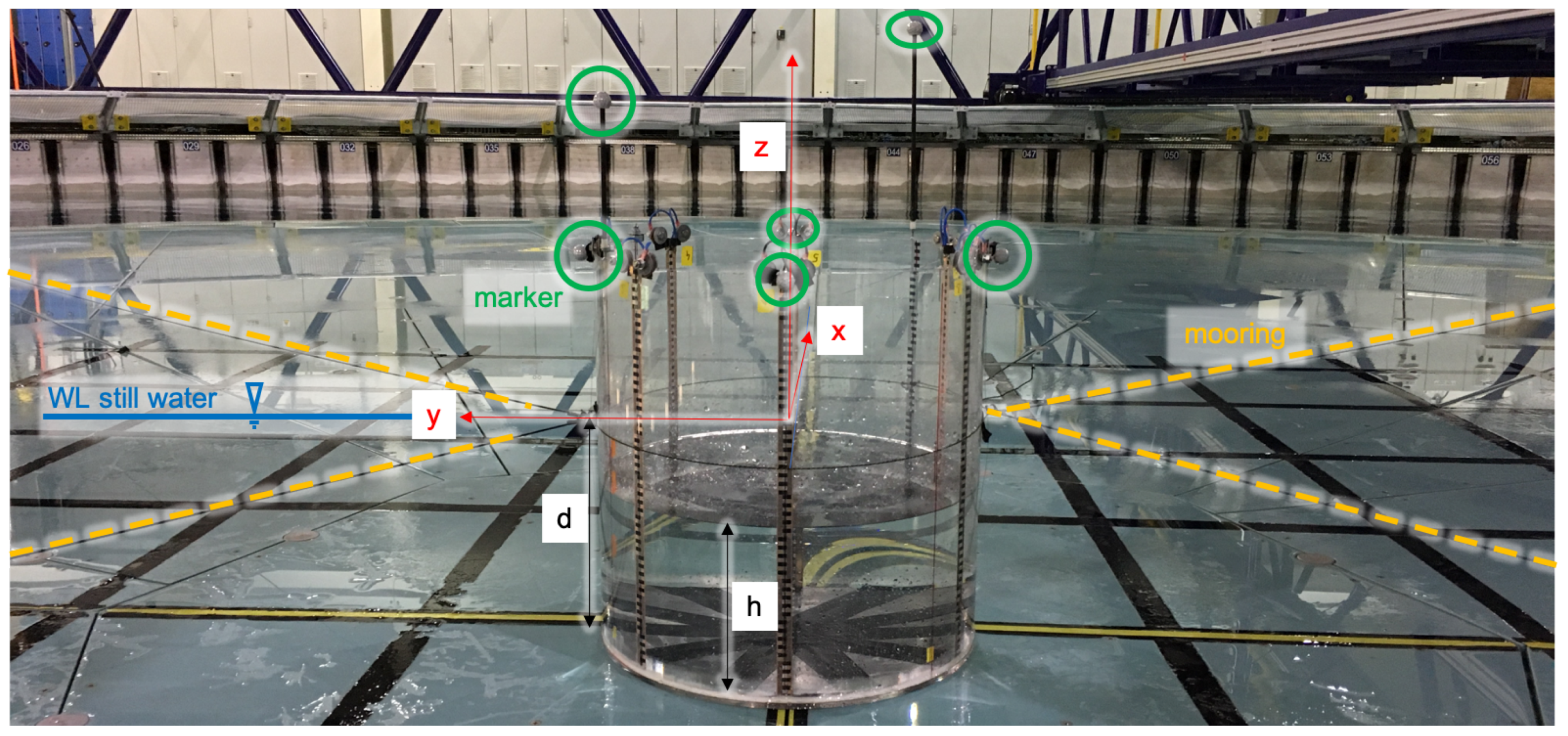
2.2. Motion Capturing System
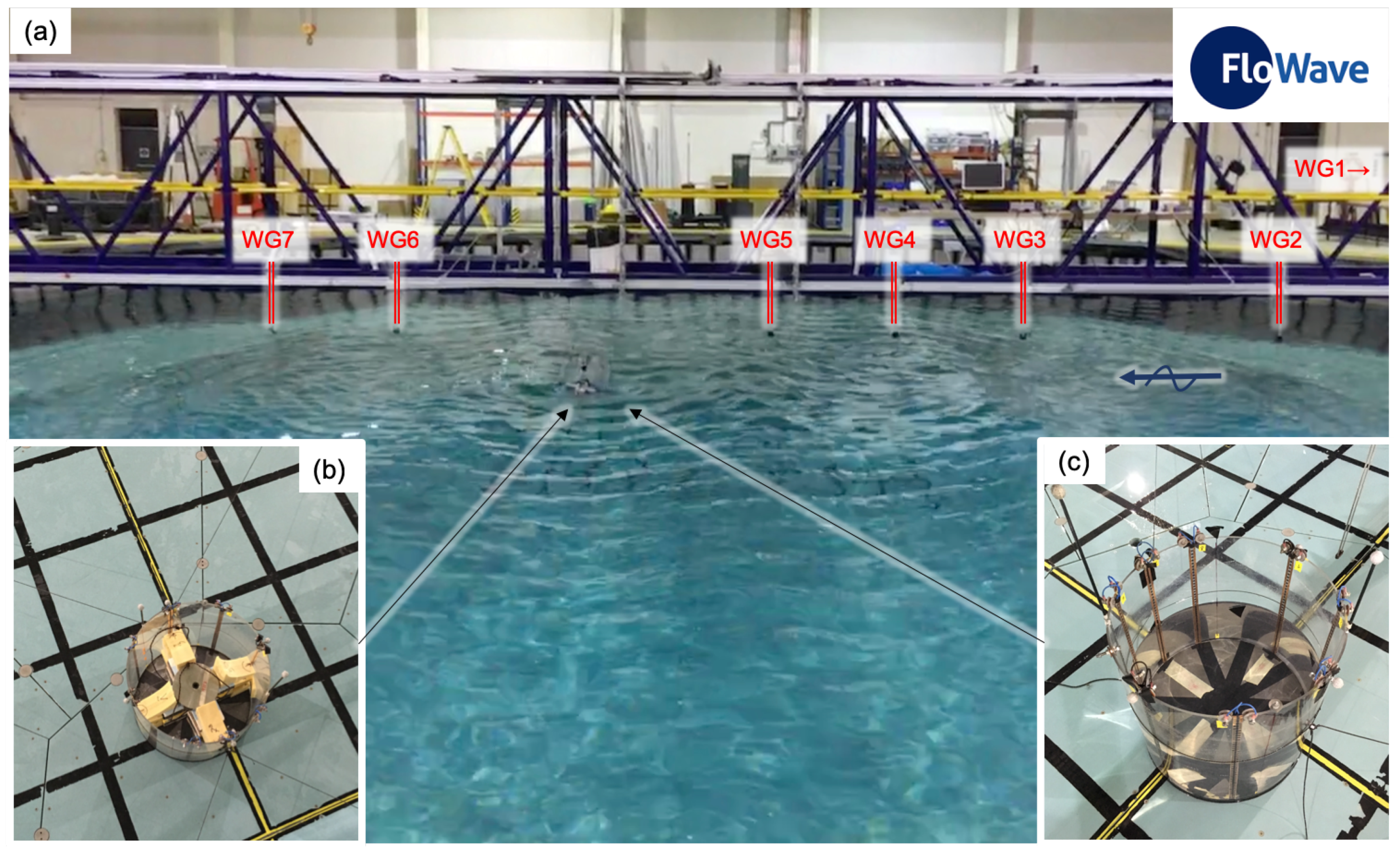
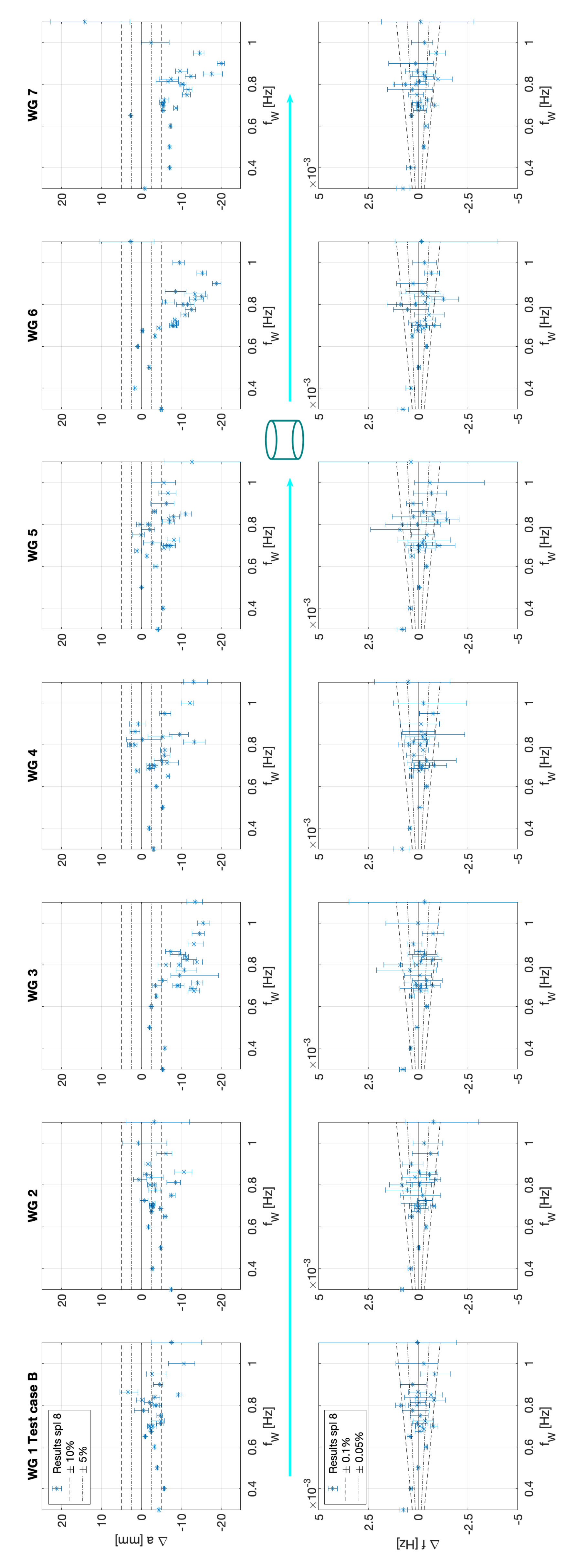
2.3. Wave Gauges
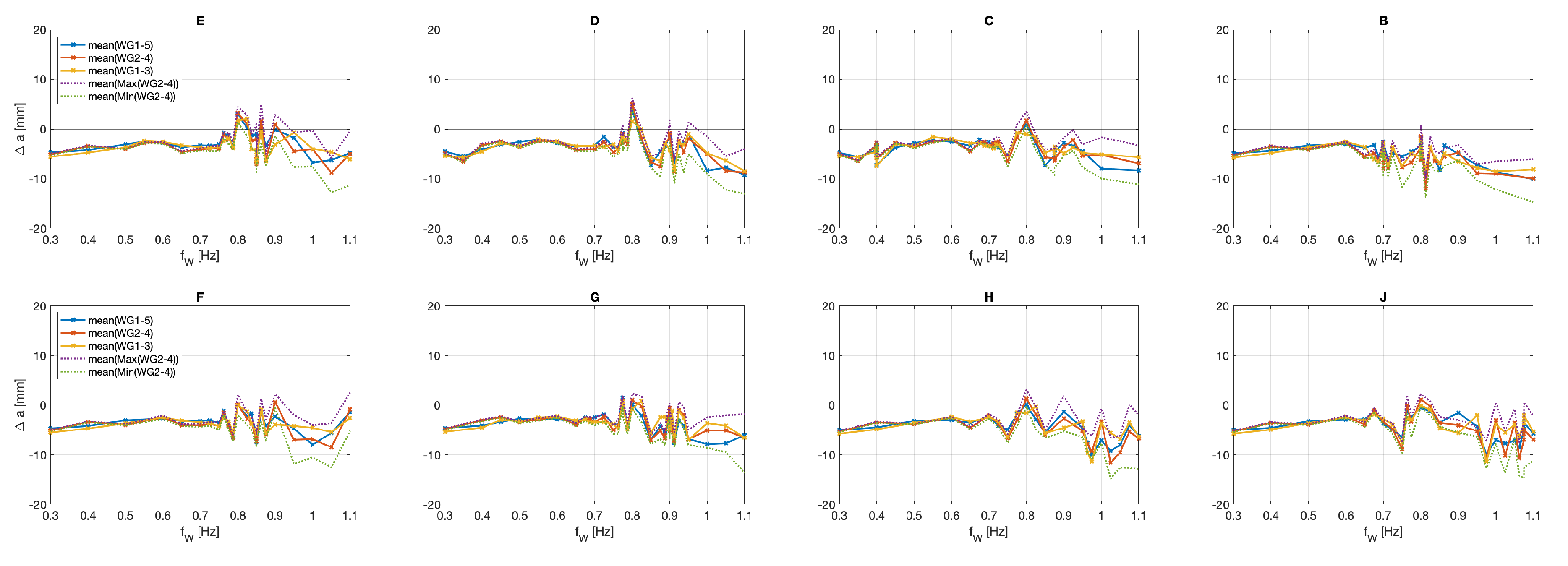
3. Dataset Description
Author Contributions
Funding
Acknowledgments
Conflicts of Interest
Notation
| a | = amplitude waves (mm) |
| = difference amplitude waves (mm) | |
| d | = draft cylinder (m) |
| D | = diameter cylinder (m) |
| f | = frequency (Hz) |
| = frequency response (Hz) | |
| = frequency wave (Hz) | |
| = difference frequency wave (Hz) | |
| g | = gravity acceleration (ms) |
| h | = water depth inside the cylinder (m) |
| H | = height of the cylinder (m) |
| WG | = wave gauge |
| WL | = water level |
| x | = distance in the main wave direction (m) |
| y | = distance orthogonal to the main wave direction (m) |
| z | = distance vertical direction (m) |
| = mass density of water ≈ 998 (kg m) |
References
- Caron, P.A.; Cruchaga, M.A.; Larreteguy, A.E. Study of 3D sloshing in a vertical cylindrical tank. Phys. Fluid 2018, 30, 082112. [Google Scholar] [CrossRef]
- Cruchaga, M.A.; Reinoso, R.S.; Storti, M.A.; Celentano, D.J.; Tezduyar, T.E. Finite element computation and experimental validation of sloshing in rectangular tanks. Comput. Mech. 2013, 52, 1301–1312. [Google Scholar] [CrossRef]
- Kim, S.Y.; Kim, K.H.; Kim, Y. Comparative study on pressure sensors for sloshing experiment. Ocean. Eng. 2015, 94, 199–212. [Google Scholar] [CrossRef]
- Lyu, W.; el Moctar, O.; Potthoff, R.; Neugebauer, J. Experimental and numerical investigation of sloshing using different free surface capturing methods. Appl. Ocean. Res. 2017, 68, 307–324. [Google Scholar] [CrossRef]
- Chen, Y.; Xue, M.-A. Numerical Simulation of Liquid Sloshing with Different Filling Levels Using OpenFOAM and Experimental Validation. Water 2018, 10, 1752. [Google Scholar] [CrossRef]
- Kim, K.-T.; Lee, P.-S.; Park, K.C. A direct coupling method for 3D hydroelastic analysis of floating structures. Int. J. Numer. Methods Eng. 2013, 96, 842–866. [Google Scholar] [CrossRef]
- Wei, W.; Fu, S.; Moan, T.; Lu, Z.; Deng, S. A discrete-modules-based frequency domain hydroelasticity method for floating structures in inhomogeneous sea conditions. J. Fluids Struct. 2017, 74, 321–339. [Google Scholar] [CrossRef]
- Yoon, J.S.; Cho, S.P.; Jiwinangun, R.G.; Lee, P.S. Hydroelastic analysis of floating plates with multiple hinge connections in regular waves. Mar. Struct. 2014, 36, 65–87. [Google Scholar] [CrossRef]
- Lee, K.H.; Cho, S.; Kim, K.T.; Kim, J.G.; Lee, P.S. Hydroelastic analysis of floating structures with liquid tanks and comparison with experimental tests. Appl. Ocean. Res. 2015, 52, 167–187. [Google Scholar] [CrossRef]
- Xu, Q.; Hu, Z.; Jiang, Z. Experimental investigation of sloshing effect on the hydrodynamic responses of an FLNG system during side-by-side operation. Ships Offshore Struct. 2018, 12, 804–817. [Google Scholar] [CrossRef]
- Zhao, D.; Hu, Z.; Chen, G. Experimental investigation on dynamic responses of FLNG connection system during side-by-side offloading operation. Ocean. Eng. 2017, 136, 283–293. [Google Scholar]
- Zhao, D.; Hu, Z.; Zhou, K.; Chen, G.; Chen, X.; Feng, X. Coupled analysis of integrated dynamic responses of side-by-side offloading FLNG system. Ocean. Eng. 2018, 168, 60–82. [Google Scholar] [CrossRef]
- Gabl, R.; Davey, T.; Nixon, E.; Steynor, J.; Ingram, D.M. Comparison of a Floating Cylinder with Solid and Water Ballast. Water 2019, in press. [Google Scholar]
- Gabl, R.; Davey, T.; Nixon, E.; Steynor, J.; Ingram, D.M. Dataset Floating Cylinder with Solid and Water Ballast; DataShare Edinburgh [Dataset]; University of Edinburgh, Institute for Energy Systems: Edinburgh, UK, 2019. [Google Scholar] [CrossRef]
- Payne, G.; Taylor, J.; Ingram, D. Best practice guidelines for tank testing of wave energy converters. J. Ocean. Technol. 2009, 4, 38–70. [Google Scholar]
- Heller, V. Scale effects in physical hydraulic engineering models. J. Hydraul. Res. 2011, 49, 293–306. [Google Scholar] [CrossRef]
- Gabl, R.; Steynor, J.; Forehand, D.I.M.; Davey, T.; Bruce, T.; Ingram, D.M. Capturing the Motion of the Free Surface of a Fluid Stored within a Floating Structure. Water 2019, 11, 50. [Google Scholar] [CrossRef]
- Draycott, S.; Noble, D.; Davey, T.; Bruce, T.; Ingram, D.; Johanning, L.; Smith, H.; Day, A.; Kaklis, P. Re-creation of site-specific multi-directional waves with non-collinear current. Ocean Eng. 2018, 152, 391–403. [Google Scholar] [CrossRef]
- Draycott, S.; Davey, T.; Ingram, D.M. Simulating Extreme Directional Wave Conditions. Energies 2017, 10, 1731. [Google Scholar] [CrossRef]
- Ingram, D.; Wallace, R.; Robinson, A.; Bryden, I. The design and commissioning of the first, circular, combined current and wave test basin. In Proceedings of the Oceans 2014 MTS/IEEE, Taipei, Taiwan, 7–10 April 2014. [Google Scholar]
- Draycott, S.; Sellar, B.; Davey, T.; Noble, D.R.; Venugopal, V.; Ingram, D. Capture and Simulation of the Ocean Environment for Offshore Renewable Energy. Renew. Sustain. Energy Rev. 2019, 104, 15–29. [Google Scholar] [CrossRef]
- Gomit, G.; Chatellier, L.; Calluaud, D.; David, L. Free surface measurement by stereo-refraction. Exp. Fluids 2013, 54, 1540. [Google Scholar] [CrossRef]
- MARINET (2012) Work Package 2: Standards and Best Practice—D2.1 Wave Instrumentation Database. Revision: 05. Available online: http://www.marinet2.eu/wp-content/uploads/2017/04/D2.01-Wave-Instrumentation-Database.pdf (accessed on 19 November 2019).
- Draycott, S.; Payne, G.; Steynor, J.; Nambiar, A.; Sellar, B.; Venugopal, V. An experimental investigation into non-linear wave loading on horizontal axis tidal turbines. J. Fluids Struct. 2019, 84, 199–217. [Google Scholar] [CrossRef]


| Weight (kg) | d (cm) | h (cm) | Solid | Water | |
|---|---|---|---|---|---|
| Cylinder | 6.25 | 3.19 | |||
| Lead | 5.46 | 2.78 | |||
| Top | 0.82 | 0.42 | |||
| dry/empty = CyEmp | 12.52 | 6.39 | 0.00 | ||
| Ballast | |||||
| Ba1 | 8.95 | 4.57 | 4.76 | ||
| Ba2 | 17.8 | 9.08 | 9.46 | ||
| Ba3 | 23.18 | 11.83 | 12.32 | ||
| Combinations | |||||
| CyEmp+Ba1+Ba2+Ba3 = | 62.45 | 31.87 | 26.53 | B | J |
| CyEmp+Ba2+Ba3 = | 53.50 | 27.30 | 21.78 | C | H |
| CyEmp+Ba1+Ba3 = | 44.65 | 22.79 | 17.07 | D | G |
| CyEmp+Ba3 = | 35.70 | 18.22 | 12.32 | E | F |
| WGNr | WG1 | WG2 | WG3 | WG4 | WG5 | Cylinder | WG6 | WG7 |
|---|---|---|---|---|---|---|---|---|
| x (m) | −8.215 | −5.692 | −3.168 | −1.904 | −0.630 | var | 3.175 | 4.443 |
| WG1-2 | WG2-3 | WG3-4 | WG4-5 | WG5-Center | Center-WG6 | WG5-6 | WG6-7 | |
|---|---|---|---|---|---|---|---|---|
| diff (m) | 2.52 | 2.52 | 1.26 | 1.27 | 0.63 | 3.18 | 3.81 | 1.27 |
| diff/ (–) | 2.0 | 2.0 | 1.0 | 1.0 | 0.5 | 2.5 | 3.0 | 1.0 |
| Run ID | Frequency Input | Amplitude Input | Degree | Frequency Wave Gauge | Amplitude Wave Gauge |
|---|---|---|---|---|---|
| [Hz] | [mm] | [] | [Hz] | [mm] |
| X | Y | Z | Yaw | Pitch | Roll | Residual | WG1 | WG2 | WG3 | WG4 | WG5 | WG6 | WG7 |
|---|---|---|---|---|---|---|---|---|---|---|---|---|---|
| [mm] | [mm] | [mm] | [mm] | [mm] | [mm] | [mm] | [mm] | [mm] | [mm] | [mm] |
© 2019 by the authors. Licensee MDPI, Basel, Switzerland. This article is an open access article distributed under the terms and conditions of the Creative Commons Attribution (CC BY) license (http://creativecommons.org/licenses/by/4.0/).
Share and Cite
Gabl, R.; Davey, T.; Nixon, E.; Steynor, J.; Ingram, D.M. Experimental Data of a Floating Cylinder in a Wave Tank: Comparison Solid and Water Ballast. Data 2019, 4, 146. https://doi.org/10.3390/data4040146
Gabl R, Davey T, Nixon E, Steynor J, Ingram DM. Experimental Data of a Floating Cylinder in a Wave Tank: Comparison Solid and Water Ballast. Data. 2019; 4(4):146. https://doi.org/10.3390/data4040146
Chicago/Turabian StyleGabl, Roman, Thomas Davey, Edd Nixon, Jeffrey Steynor, and David M. Ingram. 2019. "Experimental Data of a Floating Cylinder in a Wave Tank: Comparison Solid and Water Ballast" Data 4, no. 4: 146. https://doi.org/10.3390/data4040146
APA StyleGabl, R., Davey, T., Nixon, E., Steynor, J., & Ingram, D. M. (2019). Experimental Data of a Floating Cylinder in a Wave Tank: Comparison Solid and Water Ballast. Data, 4(4), 146. https://doi.org/10.3390/data4040146