Article

Building a SAR-Enabled Data Cube Capability in Australia Using SAR Analysis Ready Data

1
Commonwealth Scientific and Industrial Research Organisation (CSIRO) Land & Water, Canberra ACT 2601, Australia
2
CSIRO Data61, Floreat WA 6014, Australia
3
CSIRO Data61, Canberra ACT 2601, Australia
4
Geoscience Australia, GPO Box 378, Canberra ACT 2601, Australia
5
solo Earth Observation (soloEO), Tokyo 104-0054, Japan
*
Author to whom correspondence should be addressed.
Data 2019, 4(3), 100; https://doi.org/10.3390/data4030100
Submission received: 28 May 2019 / Revised: 10 July 2019 / Accepted: 12 July 2019 / Published: 15 July 2019
(This article belongs to the Special Issue Earth Observation Data Cubes)

Abstract

:
A research alliance between the Commonwealth Scientific and Industrial Research Organization and Geoscience Australia was established in relation to Digital Earth Australia, to develop a Synthetic Aperture Radar (SAR)-enabled Data Cube capability for Australia. This project has been developing SAR analysis ready data (ARD) products, including normalized radar backscatter (gamma nought, γ0), eigenvector-based dual-polarization decomposition and interferometric coherence, all generated from the European Space Agency (ESA) Sentinel-1 interferometric wide swath mode data available on the Copernicus Australasia Regional Data Hub. These are produced using the open source ESA SNAP toolbox. The processing workflows are described, along with a comparison of the γ0 backscatter and interferometric coherence ARD produced using SNAP and the proprietary software GAMMA. This comparison also evaluates the effects on γ0 backscatter due to variations related to: Near- and far-range look angles; SNAP’s default Shuttle Radar Topography Mission (SRTM) DEM and a refined Australia-wide DEM; as well as terrain. The agreement between SNAP and GAMMA is generally good, but also presents some systematic geometric and radiometric differences. The difference between SNAP’s default SRTM DEM and the refined DEM showed a small geometric shift along the radar view direction. The systematic geometric and radiometric issues detected can however be expected to have negligible effects on analysis, provided products from the two processors and two DEMs are used separately and not mixed within the same analysis. The results lead to the conclusion that the SNAP toolbox is suitable for producing the Sentinel-1 ARD products.

1. Introduction

1.1. Background

Synthetic Aperture Radar (SAR) data have been shown to provide different and complementary information to the more common optical remote sensing data. Radar backscatter response is a function of topography, land cover structure, orientation, and moisture characteristics—including vegetation biomass—and the radar signal is able to penetrate clouds, providing information about the earth’s surface where optical sensors cannot. Despite these advantages, it is not used as extensively or operationally as optical data. Reasons for this have included the traditionally high cost of SAR data acquisition and the relatively complex and specialized processing methods [1].
The release of freely available European Copernicus programme data, especially the routinely acquired global coverage of Sentinel-1 SAR data, has opened up opportunities for greater exploration and application of SAR data globally. The Sentinel-1A and 1B SAR satellites have been operating since 2014 and 2016 respectively, and have been building up an archive of dual polarized C-band data, including extensive, wall-to-wall acquisitions over Australia since December 2016 at the spatial resolution of ~3 m × 22 m in the default acquisition mode of interferometric wide (IW) swath [2].
Digital Earth Australia (DEA) is an analysis platform for observations of all forms [3], but particularly those captured from satellites which have unique potential and pose particular challenges for their full exploitation. DEA uses images and information recorded by satellites orbiting our planet to detect physical changes across Australia. DEA was originally built upon the extensive Landsat archive processed into an analysis ready data (ARD) product (including atmospheric correction to surface reflectance, co-registration, and associated cloud/cloud shadow masks), and is being developed to feature other satellite datasets including SAR. A research alliance between the Commonwealth Scientific and Industrial Research Organization (CSIRO) and Geoscience Australia (GA) was established to develop SAR capability for DEA (referred to as the Australian SAR Data Cube project).
GA and the CSIRO are also both partners in the Open Data Cube (ODC) initiative, in which ODC platforms [4] aim to enable easier access to satellite ARD, as they remove the need for the user to pre-process Earth observation datasets, and provide access to archived remotely sensed data in a format ready for use. The definition of ARD with respect to SAR data is being actively developed through the Committee on Earth Observation Satellites (CEOS) analysis ready data for land (CARD4L) framework [5]. The Australian SAR Data Cube project has been utilizing this information in developing SAR ARD products for Australia, which currently include radar backscatter (gamma nought, γ0), eigenvector-based dual-polarization decomposition and interferometric coherence, all generated from the Sentinel-1 IW swath mode data available through the Copernicus Australasia Regional Data Hub [6]. These three products have been selected since their processing methods are relatively well advanced, and they have already been used for environmental and agricultural applications within Australia [7,8]. Another reason for the selection of these three SAR ARD products for Australia is due to the availability of the dual-polarized Sentinel-1 SAR imagery by the European Space Agency (ESA).
The processing workflows for producing these SAR ARD products make use of ESA’s free Sentinel-1 Toolbox within the Sentinel Application Platform (SNAP). SNAP is an open source platform, allowing easy access and sharing of processing workflows with the capability of batch processing through its graph processing tool (GPT). To evaluate the performance of SNAP for producing SAR ARD products, selected scenes are also processed to radar backscatter and interferometric coherence using the proprietary software GAMMA [9] for comparison.
This manuscript first describes the three SAR ARD products being developed for the Australian SAR Data Cube project and the applications they have been used for, with particular emphasis on Sentinel-1. It then details the workflows used to produce the SAR ARD products using the SNAP toolbox and gives an example of how the three selected products provide complementary information about the landscape. We then evaluate the outputs from the SNAP toolbox and compare them to outputs from the proprietary GAMMA software.

1.2. SAR ARD Products

The Australian SAR ARD products are currently produced using Sentinel-1 data in IW swath mode, which has been acquired systematically since October 2014 (for Sentinel-1A). It covers a swath of 250 km at a spatial resolution of ~3 m × 22 m (single look complex–SLC), or 20 m × 22 m for its ground range detected (GRD) high resolution class (HR) sampled to 10 m × 10 m, allowing regional coverage at a pixel size compatible with optical sensors such as the Landsat data series. Each Sentinel-1 satellite carries a dual polarization C-band SAR sensor (i.e., switchable H or V transmitter and parallel H and V receivers). Over land it is typically configured to acquire VH (vertical transmit–horizontal receive) and VV (vertical transmit–vertical receive) polarizations in IW mode [2]. Sentinel-1A in conjunction with Sentinel-1B have been routinely acquiring the dual-polarimetric IW products across the whole of Australia every 12 days since December 2016.
The SAR ARD products being developed for an Australian SAR data cube are normalized radar backscatter, dual-polarization decomposition, and interferometric coherence. These products are currently being tested for integration into the DEA data cube (which is part of the ODC initiative), which involves indexing of the products and retaining relevant metadata information to meet CARD4L standards. The normalized radar backscatter is the most widely used, however there are advantages to including the dual-polarization decomposition and interferometric coherence in a range of applications. These will be demonstrated in the following sections, based on information available in the literature, as well as an example of some SAR ARD data for Australia.

1.2.1. Radar Backscatter

Radar backscatter is the most widely used of the SAR products due to it being the simplest to produce and understand. It typically gives the proportion of radar signal backscattered to the receiver as amplitude (or intensity). Radar backscatter is dependent on the characteristics of the surface it is interacting with including its dielectric properties, orientation, and structure [10].
Applications based on SAR backscatter have appeared extensively for decades including a range of applications such as mangrove monitoring [11], forest biomass [12], and flood extent mapping [13,14]. However, the availability of free SAR archive data has increased the use of SAR for multi-temporal analysis, often improving results compared to single-date scenes [8]. Multi-temporal Sentinel-1 SAR can be used to identify patches of deforestation based on the detection of radar shadows from two viewing angles (using Sentinel-1 in ascending and descending mode) [15]. It has also been used to map fire scars in areas where persistent cloud-cover hampered efforts with optical remote sensing technology [16], as well as for the identification of irrigated agriculture [17].

1.2.2. Dual-Polarimetric Decomposition

For a fully polarimetric SAR system, quad-polarimetric decompositions enable the scattering mechanisms to be extracted as a single scattering matrix from the averaged Mueller matrix, decomposed into the sum of elementary matrices from the coherent scattering matrix, or characterized into physical scattering mechanisms by eigenvector-based decompositions of the coherency or covariance matrix [18]. These methods are used to distinguish land cover types exhibiting different scattering behaviors. Since the default imaging mode (IW) of Sentinel-1 works with selectable dual polarization, the quad-polarizations are not available. However, eigenvector-based dual-polarimetric decomposition can be applied to characterize the behavior of the scatterers to a certain extent, resulting in entropy, anisotropy, and alpha parameters [19].
This information is useful in applications such as land cover classification and change detection analysis. Zhou et al. [8] demonstrate how including the dual-polarimetric decomposition bands (entropy, anisotropy, and alpha) along with the normalized radar backscatter of multi-temporal Sentinel-1 data improves the discrimination of dryland crop type in the Wheatbelt of Victoria, Australia, as well as detecting the growth stage of an irrigated rice region in New South Wales. Cloude [19] demonstrates the ability of entropy/alpha in discriminating forest from non-forest, and in highlighting the complex scattering behavior of urban environments.

1.2.3. Multi-Temporal Coherence

Multi-temporal (or interferometric) coherence is a by-product when generating interferograms for applications such as deformation monitoring. However interferometric coherence can also be useful for determining whether the scattering properties of a surface change through time. This can be related to land-cover change or vegetation growth. The coherence between two images reduces over time as the land surface changes, which is more pronounced for the shorter wavelengths (such as C-band). This is particularly so for vegetation cover. However, objects that do not change through time (or change very slowly) can have a high coherence value between two multi-temporal images. In particular, buildings or bare ground (with constant soil moisture) can have a high coherence compared to their surroundings [20]. Sentinel-1 interferometric coherence is of interest to the ESA as demonstrated through the SINCOHMAP project [21], which is developing methods for land cover and vegetation mapping. Tamm et al. [22] found it was feasible to use Sentinel-1 12-day repeat pass interferometric coherence for identifying the dates that grasslands have been mown. However ploughed fields and remnant grass created confusion. One of the challenges of using interferometric coherence is that precipitation can cause temporal decorrelation [22].

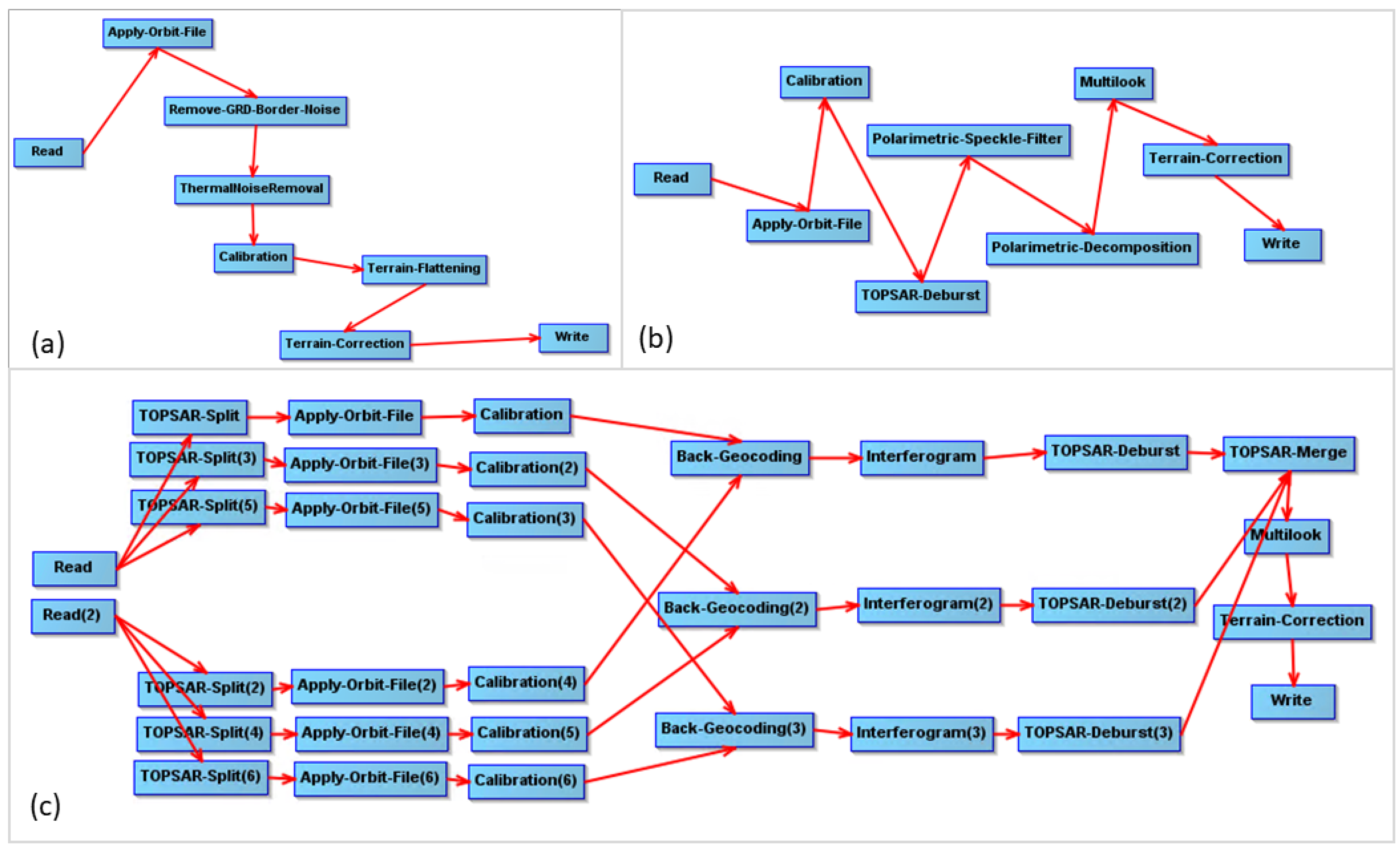
2. SNAP Graph Processing Tool Workflow

2.1. SNAP Processing

The code developed in the SAR data cube project comprises a collection of shell scripts and python code to enable batch processing of the SNAP graph processing tool (GPT) XML files [23]. To produce a SAR ARD product, the list of available Sentinel-1 files is first extracted through the Sentinel Australasia Regional Access (SARA) portal [24]. SARA’s web API allows queries based on area of interest, date range, Sentinel-1 level-1 data type (GRD or SLC), and sensor mode (in this case IW is used). The GPT executable is then run using the GPT graph XML files on the list of Sentinel-1 zip files. This process is currently run on the Australian National Computational Infrastructure [25], the same facility hosting SARA, so no data transfer is required for Sentinel-1 level-1 data access.
While each SAR ARD product requires its own processing workflow, some common steps and parameters are used for all. For IW mode, Sentinel-1 acquires data in three sub-swaths (and numerous bursts that are synchronized between passes) using the TOPSAR (terrain observation with progressive scans SAR) method [26]. To form a complete image from the SLC data, each sub-swath needs to be processed, including ‘debursting’ to remove the gaps between each burst, and then merged together [2]. Precise orbit file correction is applied to each SAR ARD product to ensure best geo-positional accuracy. All SAR ARD products are geometrically corrected using the ‘SRTM 1Sec HGT’ option available in the SNAP toolbox, which is automatically downloaded within the processing, or using the pre-downloaded and/or refined SRTM 1 arc-second DEM as a local DEM. The Australian Albers equal area projection was selected for the SAR ARDs, ensuring interoperability with the extensively used Landsat ARD products in DEA. An output pixel size of 25 m × 25 m is used for compatibility with the DEA Landsat series. The current output format is the BEAM-DIMAP flat binary image file format, as it is the native output by SNAP. However, GeoTIFF image file format, with internal compressed tiling enabled, is preferred as it improves compatibility with other software tools and improves performance (e.g., windowed reading). Conversion from BEAM-DIMAP to compressed GeoTIFF file format is performed after the initial SAR ARD product is created.
Each SAR ARD workflow is now described in more detail as it is processed in SNAP. Each of the processing steps, as built in the SNAP graph builder tool, is shown in Figure 1. All processing parameters are left as their default option unless specified.
The normalized radar backscatter ARD is gamma nought (γ0) as recommended in the CARD4L report [27], since it accounts for topographic variation better than the more traditional sigma naught (σ°) [28]. This ARD is generated from the ESA’s Sentinel-1 GRD product, rather than the SLC product, to save on processing time since debursting and multi-looking have already been applied [29]. It requires removal of border noise along the edge of some scenes, where the ‘borderLimit’ is set to 800 pixels, and the ‘trimThreshold’ to 10.0, to correct for some of the early Sentinel-1 scenes that had a wide strip of border noise with relatively high intensity values. Thermal noise removal is applied, before the image is calibrated to γ0 backscatter. Radiometric terrain flattening is then applied using the ‘SRTM 1Sec HGT’ product available in SNAP, followed by the range Doppler terrain correction to orthorectify the image. The local incidence angle image is also output to meet CARD4L recommendations. No speckle filtering is applied to the radar backscatter SAR ARD product, as the type and parameters for speckle filtering (if one is required) is determined by its application.
The dual-polarization decomposition SAR ARD is generated from ESA’s Sentinel-1 SLC product. The image is calibrated, but kept in complex format, and then deburst. The improved Lee Sigma filter is applied as it results in a smoother output image, before the H-alpha dual-polarization decomposition step to generate the alpha, anisotropy, and entropy bands. Each band is then multi-looked to create square pixels, before range Doppler terrain correction to orthorectify the image.
Processing the Sentinel-1 data into an interferometric coherence product first requires the matching of suitable interferometric scene pairs. For the interferometric coherence ARD product, scenes are considered as a suitable pair for processing if they have the same relative orbit number, and their acquisitions are a maximum of 12 days apart. Once the image pairs are defined and precise orbit correction applied, radiometric calibration is applied, followed by back-geocoding to each sub-swath before an interferogram is generated. The window size used for estimating coherence when generating the interferogram is set at 30 pixels in the range direction, and 9 pixels in azimuth, to produce a smoother output image. The flat-earth (reference) phase is subtracted in this step to remove the effects of the earth’s curvature. The sub-swaths are then deburst and merged into a single image, followed by multi-looking and range Doppler terrain correction to orthorectify the image.
The batch processing of Sentinel-1 data to ARD for backscatter, dual-polarimetric decomposition, and interferometric coherence has been automated for execution on the Raijin super-computer at the National Computational Infrastructure (NCI, http://nci.org.au/). The code used to process the Sentinel-1 data on the NCI is available on the GitHub: https://github.com/opendatacube/radar. One complication of running the processing on high-performance facilities at the NCI is that the compute nodes do not have an external network interface. In the SNAP processing sequences discussed above, this creates issues when some of the steps are set to automatically download data from the ESA servers. This mainly applies to the apply-orbit-file, terrain-correction and back-geocoding steps, which require access to external orbit files or tiles of digital elevation model (DEM) data. To circumvent this issue, the necessary files of external data are pre-downloaded to the NCI file system prior to processing, and the SNAP workflow is made to use these files during execution.
Python code is used to submit jobs to Raijin to process the Sentinel-1 files as per the user’s specifications (date range, spatial extents, etc.). Processing of the XML workflow using the GPT occurs in a multi-threaded way, allowing each job to be executed on multiple computer processing units (CPUs). Typical processing times (‘walltime’, using 8 CPUs) required by the tasks of interest are:
  • Backscatter: 30–40 min per scene with typical input scene sizes of 0.5 Gb to 1 Gb.
  • Dual-polarimetric decomposition: 80–85 min per scene with typical input scene sizes of 4.5 Gb.
  • Interferometric coherence: 55–65 min per pair of Sentinel scenes with typical input scene sizes of 4.5 Gb.

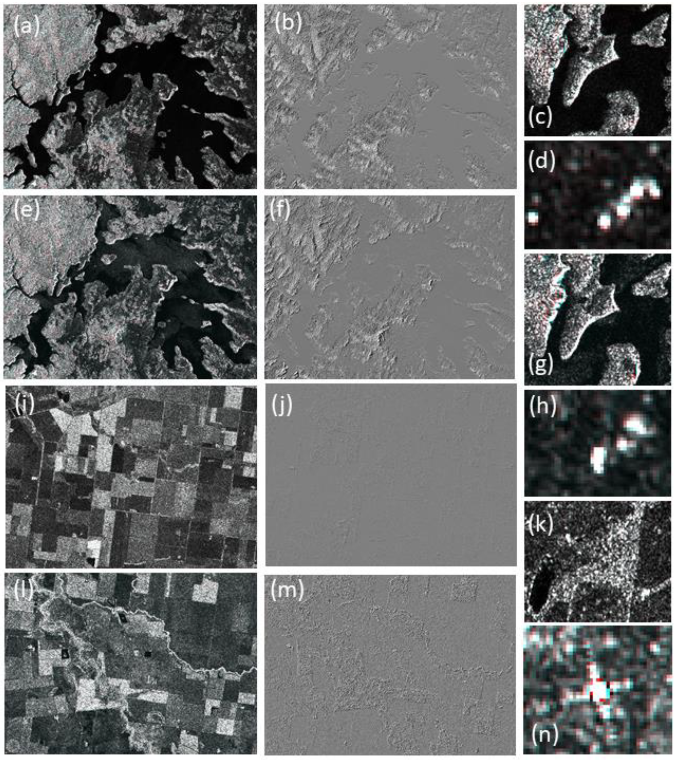
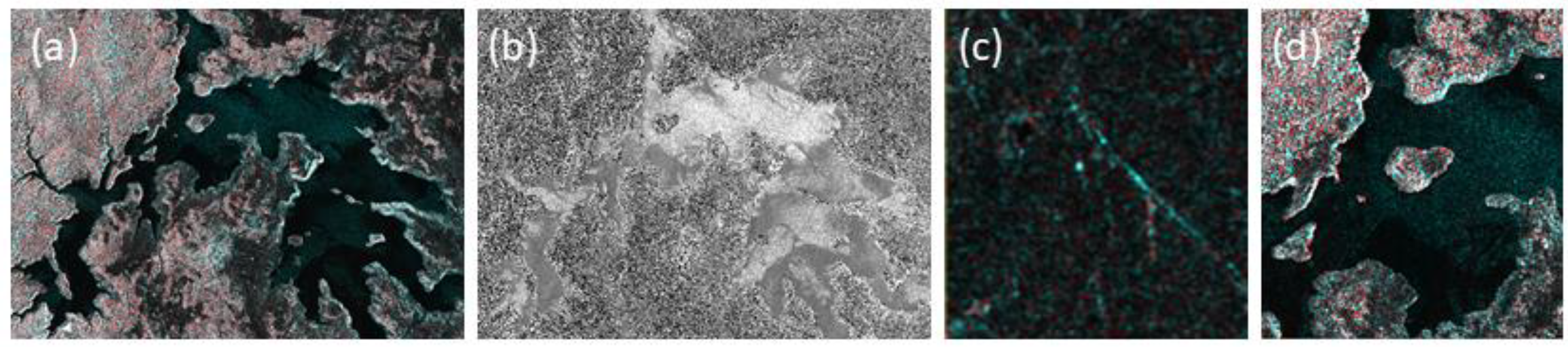
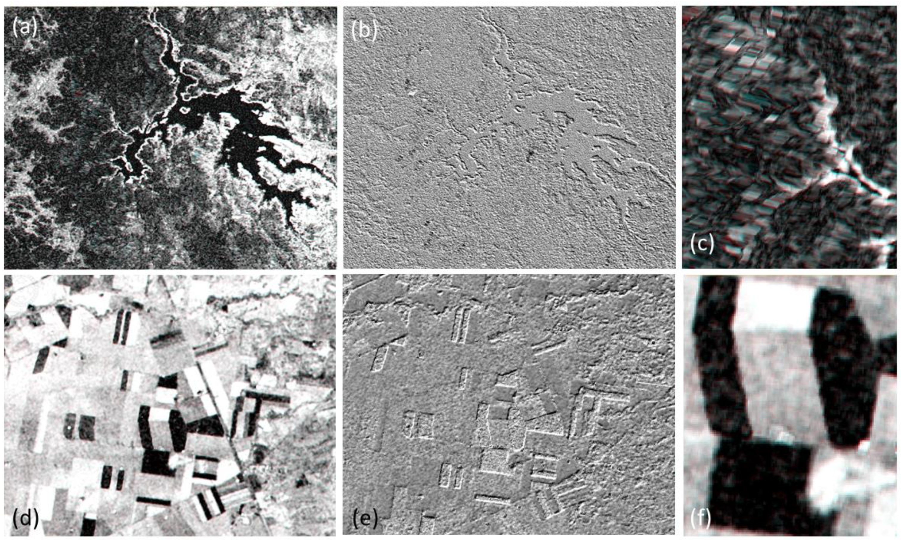
2.2. Demonstration of SAR ARD Products

Normalized radar backscatter is often used in SAR applications, while dual-polarimetric decomposition and interferometric coherence are less common. However, depending on the application, there are benefits in using more than one of the ARD products. The benefits of utilizing the normalized radar backscatter, dual-polarimetric decomposition, and interferometric coherence are shown within the coastal zone of the Fitzroy River catchment in Western Australia.
Sentinel-1A data were processed to all three ARD products described in Section 2.1 for the Fitzroy River catchment (Figure 2) for December 2016 to April 2017. Sentinel-2 data were also used for a similar date (based on cloud cover) to identify land cover. The radar backscatter also had a Lee Sigma speckle filter applied to reduce speckle effects.
Figure 2 shows the γ0 VV, γ0 VH, entropy and interferometric coherence bands for three dates, along with a cloud-free Sentinel-2 scene. This scene shows a tidal inlet surrounded by mudflats and coastal mangroves. The middle of the scene consists of mangroves within the intertidal zone with larger mangroves adjacent to narrow river channels and the smaller mangroves and hypersaline areas further inland. The eastern side of the scene is outside the intertidal zone and consists of scattered trees among the grassland. The VH backscatter (Figure 2c) contrasts the very low backscatter of the mudflats with the high backscatter of the mangroves along the narrow channels. The VV backscatter (Figure 2b) shows further detail within the mudflats (blue areas along the lower-middle of the scene) as well as over water. The entropy band (Figur 2e) provides additional information with flooded wetlands and vegetated sand banks having a high entropy value, and the exposed non-vegetated sand banks having a low entropy value. This contrasts with the VV backscatter which has a low backscatter over water, but a high backscatter for the vegetated sand banks. A temporally flooded area towards the south-east of the scene (green area in Figure 2e) is not visible at all in the radar backscatter. Figure 2f demonstrates how the multi-temporal interferometric coherence can provide additional information in an environment as complex as a mangrove coastal zone. The information shown in the interferometric coherence image (Figure 2f) is very different to that available in the backscatter images (Figure 2b,c). High interferometric coherence values are observed over the slightly elevated bare areas within the coastal zone that aren’t subject to tidal flooding.

3. Assessment of Suitability of SNAP Toolbox for Australian SAR Data Cube Applications

To test how robust the proposed method of producing Sentinel-1 SAR ARD data is, an evaluation was done comparing the proposed workflow (SNAP toolbox and its default SRTM DEM from NASA’s Shuttle Radar Topography Mission [30]) to some of the best available options (proprietary GAMMA software and a refined DEM). The SNAP toolbox has the advantage in that it is open source with a relatively simple processing workflow, while the proprietary GAMMA software is widely used for specialized SAR processing. The standard SRTM DEM available in the SNAP toolbox is openly available and automatically downloaded during the processing workflow, however the refined DEM [31] is a refined version of the SRTM DEM with Australia-wide coverage. The refined DEM has void filling, vegetation removal, and smoothing applied to reduce noise associated with low relief areas. The aims of these comparisons were to:
-
Test how well the SNAP processing software compares to the proprietary GAMMA software (often considered to be one of the most reputable and industry best SAR software) when producing Sentinel-1 γ0 backscatter.
-
Compare how the standard SRTM DEM available in the SNAP processing software (referred to as the SRTM_DEM) and the refined, Australia-wide DEM (referred to as the GA_DEM [31]) influence γ0 backscatter.
-
Compare γ0 backscatter from SNAP and GAMMA in an area of relatively steep topography and an area of relatively flat terrain.
-
Compare the effects of look angle from a far-range and near-range image over the same area on the Sentinel-1 γ0 backscatter.
-
Evaluate the absolute geometric accuracy of the γ0 images based on the location of a corner reflector within a scene.
-
Compare the interferometric coherence ARD product generated from SNAP to the one generated from GAMMA.
Two study sites used for these comparisons are:
-
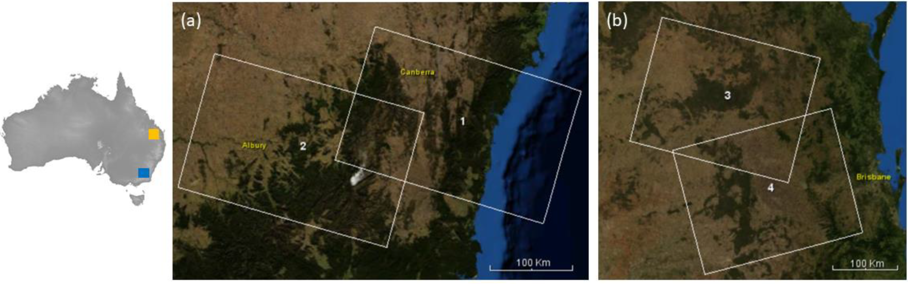
Lake Eucumbene (Figure 3a), an area in the alpine region of southeast Australia containing relatively steep topography (height differences of ~1120 to 1550 m AHD) where the orbit paths overlap to give a near- and far-range image; and
-
The Surat Basin (Figure 3b), a topographically flat (height differences of ~320 to 480 m AHD) dryland agricultural area in eastern Australia. This site is also used for radiometric and geometric calibration of SAR satellites including the Sentinel-1 constellation, through a permanent corner reflector array deployed there [32].
The Sentinel-1 images processed to γ0 backscatter for these two study sites are shown in Table 1. Two Sentinel-1 image pairs were used for generating the interferometric coherence (shown in Table 2). The processing steps and parameters used in the GAMMA software were selected to be the same as those in SNAP. There may however be slight differences due to the internal settings for some functions, which are not visible to the user. Note that a comparison could not be performed for the dual-polarimetric decomposition method, as it is only available within SNAP, not GAMMA.
The assessment is divided into four sections: Comparison of the γ0 image from the SNAP toolbox and GAMMA software; comparison of the γ0 image from the SRTM_DEM and GA_DEM; comparison of the γ0 image from the near range and far range; and comparison of the interferometric coherence image from the SNAP toolbox and GAMMA software. These sections evaluate the radiometric and geometric consistencies of the different software, DEMs, and viewing angles. Note that all Sentinel-1 scenes are VV, with the exception of a scene in the Surat Basin, which is HH. This is a Sentinel-1B scene in ascending mode, which was selected to assess the γ0 image’s absolute geometric accuracy due to the availability of an accurately characterized corner reflector within this scene [32].

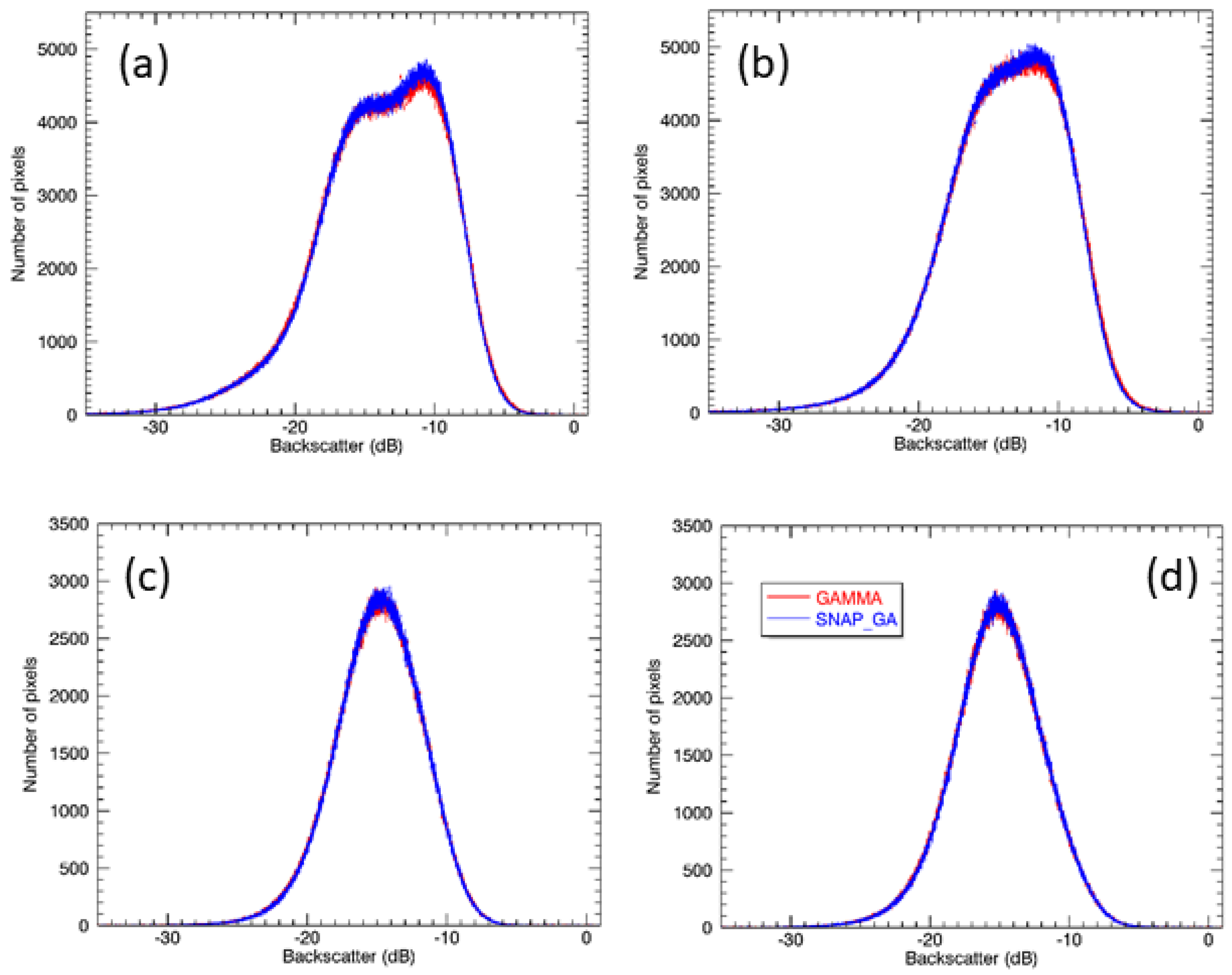
3.1. Comparison of SNAP and GAMMA Output for Radar Backscatter

GAMMA and SNAP software were used to produce radiometrically terrain corrected Sentinel-1 γ0 backscatter products for Lake Eucumbene and Surat Basin study sites, both using the same input parameters and the same DEM (the refined GA_DEM). Figure 4 shows the γ0 backscatter output for Lake Eucumbene from the far-range (top row) and near-range (middle row) images, as well as the Surat Basin (bottom two rows with HH along the bottom row) as produced from the GAMMA software and SNAP toolbox. The first column of Figure 4 shows the γ0 images from GAMMA in the red band and SNAP in the blue/green bands (i.e., cyan). The grey color of these images illustrates there is generally similar radiometric and geometric agreement between the GAMMA and SNAP γ0 backscatter products. The middle column of Figure 4 shows the GAMMA minus SNAP difference images. The geometric features visible in the difference images indicate systematic (rather than random) differences in image geometry. These differences are most prominent in areas with steep terrain and layover/radar shadowing effects (as illustrated in the GAMMA–SNAP difference images of Figure 4b,f), with shifts of 3–4 pixels detected. In terrain with moderate topography displacements in the order of 1–2 pixels were observed. In both cases the directions of the displacements furthermore differ systematically depending on the slope aspects relative to the radar, indicating different radiometric terrain correction approaches between GAMMA and SNAP. On slopes facing away from the radar a backscatter difference of 0.1 to 0.4 dB (with GAMMA values greater than SNAP) was observed compared to no detectable difference on the sides facing the radar. The magnitude of the effect was larger in the far-range image pair. The open farmlands to the east of Lake Eucumbene have backscatter intensity values within 0.1 dB. The flat agriculture areas of the Surat Basin study site show good agreement, with minor differences over vegetated areas (Figure 4m).
Figure 4c,g show a close up of the near range and far-range images respectively, including part of the lake. This area contains relatively steep terrain leading to the water’s edge. Most of this area shows good radiometric and geometric agreement, except along small sections of the water’s edge where SNAP γ0 backscatter values are higher (showing in cyan tones). The near-range image in Figure 4g includes minor differences where γ0 backscatter from GAMMA is higher than from SNAP (red tones). This occurs within a forested area adjacent to the banks of the lake. In flat open farmland, isolated buildings act as point scatterers as seen in the far range and near range (Figure 4d,h respectively), illustrating a small but systematic geometric difference between the GAMMA and SNAP outputs of less than one pixel in the north-south (azimuth) direction.
In the descending image over the Surat Basin study site (Figure 4i), small systematic differences between the GAMMA and SNAP γ0 backscatter values are visible (Figure 4j). A close-up of a local dam and forest areas (Figure 4k) show no visible difference. The ascending image (HH polarization) over the Surat Basin study site (Figure 4l) shows minor differences (Figure 4m) particularly along the vegetated river bank. A close-up of the corner reflector in Figure 4n shows that the geometric difference between the GAMMA and SNAP scenes is approximately one pixel in the east-west (range) direction. The absolute geometric accuracy of the γ0 HH image agrees to 0.8 arc-second (which is within a Sentinel-1 pixel) when compared to the coordinates of the corner reflector for both GAMMA and SNAP.
The frequency histograms of the backscatter intensity values (in dB) from Figure 4 are shown in Figure 5: For Lake Eucumbene for far range (Figure 5a), near range (Figure 5b), and the Surat Basin study site descending (Figure 5c) and ascending (Figure 5d) both of which have a mid-range look angle. Overall the results are similar, however the GAMMA output (red line) has a lower number of mid-range backscatter intensity pixels (~ −15 to −10 dB) compared to the SNAP output products (blue line). This effect occurs irrespective of radar look angle, however the differences are lower in the Surat Basin images (Figure 5c,d).
The GAMMA–SNAP difference images (middle column of Figure 4) have low mean absolute values varying from 0.013 × 10⁻³ to 1.3 × 10⁻³ intensity, with the SNAP image lower than the GAMMA processed image except for the near-range image of Lake Eucumbene (Table 3). (Note that a small number of pixels (<0.005%) behaved as strong point scatterers resulting in very high backscatter intensity values. These were masked as they incorrectly influenced overall image statistics). The standard deviation of the difference image is lowest for the Surat Basin study site in descending mode and highest for the far-range difference image of Lake Eucumbene.

3.2. Comparison of SNAP Output Using SRTM_DEM and GA_DEM for Radar Backscatter

SNAP software was used to produce Sentinel-1 γ0 images using the SRTM_DEM and GA_DEM for Lake Eucumbene and Surat Basin study sites; all used the same input parameters except for the DEMs. Figure 6 shows the γ0 backscatter output for Lake Eucumbene from the far-range (top row) and near-range (middle row) images, as well as the Surat Basin site (bottom two rows with HH along the bottom row) as produced from the SNAP toolbox with the different DEMs. The first column of Figure 6 shows the γ0 images produced using the SRTM_DEM in the red band and using the GA_DEM in the blue/green bands (i.e., cyan). The grey colour of these images illustrate similar γ0 backscatter products, both in radiometric and geometric quality. The middle column of Figure 6 shows the difference images as produced from SNAP using the SRTM_DEM and GA_DEM. The relief patterns visible in Figure 6b,f illustrate a systematic shift between the two DEMs of 1–2 pixels in the east–west (range) direction and 0.5–1 pixels in the north–south (azimuth) direction within the moderate and steep terrain. Across the lake surface and immediate shorelines, the two DEMs are identical and consequently, there are no observable differences in backscatter.
Figure 6c,g show the same close-up view around the edge of Lake Eucumbene as Figure 4c,g. As expected, the main difference in backscatter occurs in areas where the two DEMs are different. This is mostly along the edge of forested areas next to the lake, where the refined GA_DEM has been corrected to ground level (and hence tall vegetation has been removed). As a direct effect from the geometric displacement between the DEMs, the γ0 backscatter produced using the SRTM_DEM has a higher backscatter intensity along the edges of the forest facing towards the radar. The close-up view of flat open farmland near Lake Eucumbene (Figure 6d,h) shows that the geometric agreement between the SRTM_DEM and GA_DEM are within a pixel.
For the Surat Basin study site in descending mode, the main differences occur along the edges of forests (Figure 6k), similar to the Lake Eucumbene area. A close-up view of the corner reflector in the ascending image (bottom-left of Figure 6n) shows the geometric difference between the SRTM_DEM and GA_DEM is within a pixel.
The SRTM–GA DEM difference images (second column of Figure 6) have absolute mean values close to zero, with small variations observed (0.1 × 10⁻³ intensity or less, Table 4) being a direct a consequence of the geometric shift between the SRTM and GA DEMs.

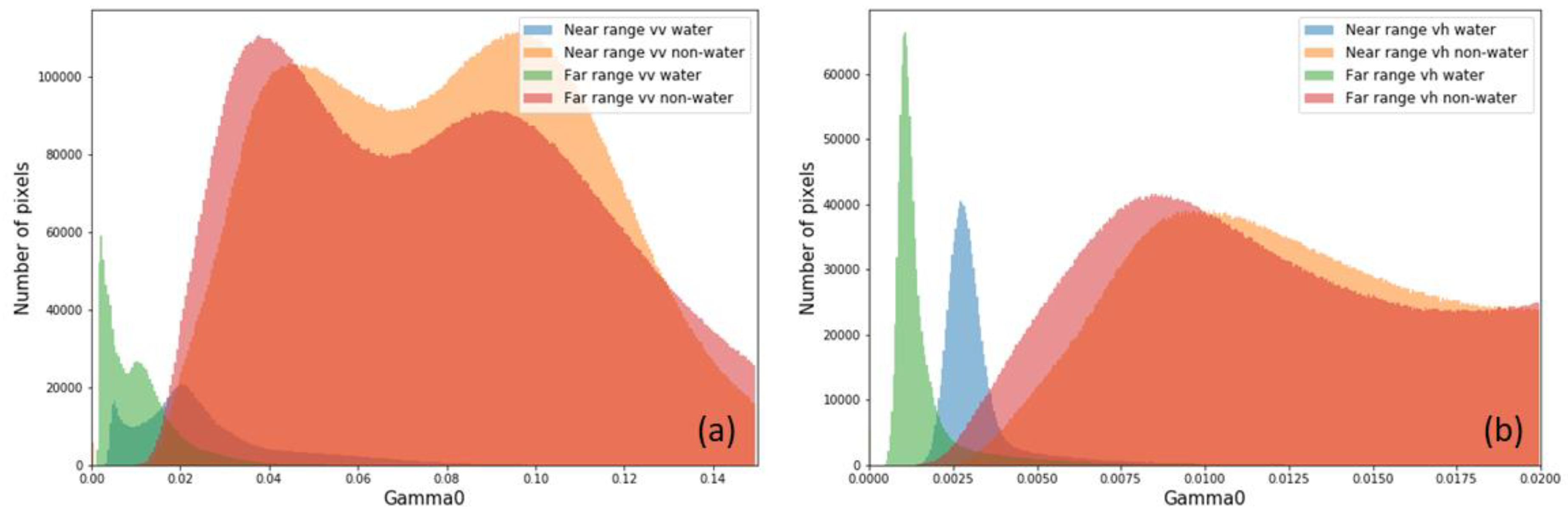
3.3. Comparison of Near-Range and Far-Range Effects for Radar Backscatter

Another important factor to consider when using multi-temporal Sentinel-1 ARD products relates to radiometric and geometric variation between the near-range and far-range images processed with the same processor. Figure 7a shows Lake Eucumbene with far range in red and near range in cyan, and Figure 7b shows the difference image. Differences on land appear random and caused by actual incidence angle differences, with no systematic geometric shifts detected. The forested areas of relatively steep terrain show higher backscatter intensity values in the far-range compared to the near-range image. Patterns are visible on the lake (with the near range having higher backscatter intensity values), which are caused by surface condition variations between the two acquisition dates (an interval of 5 days). The mean and standard deviation in intensity for this difference image are −2.5 × 10⁻³ and 0.07 respectively, which is a larger standard deviation than seen in the GAMMA–SNAP and DEM comparisons. However, the geometric accuracy between the two images is within a pixel.
Figure 7c shows a closeup of the backscatter from far-range (red) and near-range (cyan) images for an area of relatively flat farmland. The bitumen road is easily visible in the near-range (cyan), but is not visible in the far-range image due to the low backscatter return from specular scattering. There are radiometric differences between the far-range and near-range images, most likely due to the different look angles resulting in different interactions between the radar and land surface.
This difference has a direct impact on surface water mapping. Figure 7d shows a close-up view of Lake Eucumbene. There is good geometric agreement between the two dates and look angles, since the boundary between water and land match well. The blue tones within the water indicate higher backscatter in the near range over water. This can lead to confusion when discriminating water from non-water based on threshold values. Figure 8 shows histograms generated from multiple pairs of near- and far-range Sentinel-1 observations, where water and non-water pixels are identified using Landsat 8 spectral classifications (the water observations from space [33]) acquired within 5 days from corresponding Sentinel-1 scenes. The figure illustrates consistently better separation between water and non-water at larger look angles, regardless of variation caused by weather conditions (e.g., waves).
Other factors influencing the use of overlapping Sentinel-1 images relate to changes in the land surface (e.g., soil moisture) or atmospheric effects (such as heavy rain which can influence the C-band wavelength). In this study, we have particularly selected two pairs of data acquired in the dry season with lower chance of meteorology impact, however these factors need to be considered when using multi-temporal SAR ARD for environmental and agricultural applications.

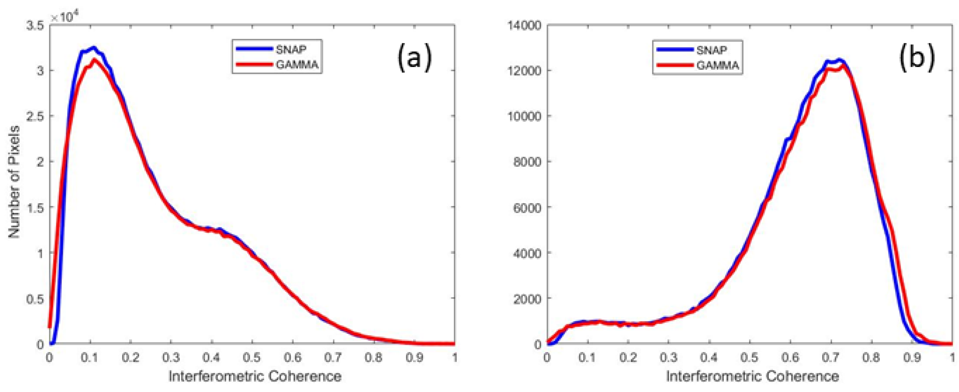
3.4. Comparison of SNAP and GAMMA Output for Interferometric Coherence

GAMMA and SNAP software were used to produce Sentinel-1 interferometric coherence products for the Lake Eucumbene and Surat Basin study sites, both using the same input parameters and the same DEM (the SRTM_DEM). For SNAP, the method used to generate interferometric coherence is shown in Section 2.1. The left-hand column in Figure 9 shows the two interferometric coherence images with SNAP in red and GAMMA in cyan, with Lake Eucumbene along the top row and the Surat Basin along the bottom. The SNAP–GAMMA coherence difference images are shown in the middle column.
For the Lake Eucumbene scene (Figure 9a), bare areas have a high coherence (white) along the eastern side of the lake. The shoreline around the lake also has a high coherence as it is void of vegetation. Coherence within the lake is very low due to decorrelation of water surface over time. There is a 0.5–1 pixel shift between the SNAP and GAMMA coherence images, with the GAMMA coherence image to the northeast of the SNAP coherence image. The greatest difference in coherence between SNAP and GAMMA occurs in steep terrain due to this systematic pixel shift and the effects of layover. This difference is greatest along the steep barren slopes around the edge of the lake, possibly due to misalignment, and forested slopes along the western side of Lake Eucumbene (Figure 9c), where gradients up to 50% result in radar shadow and layover effects.
For the Surat Basin, bare fields have a high coherence (white), and the higher-biomass crops have a very low coherence (Figure 9d). There is an approximate 1 pixel shift in this scene image with the GAMMA coherence image northeast of the SNAP coherence image. This effect is visible in the SNAP–GAMMA interferometric difference image (Figure 9e), where the greatest difference occurs along the crop edges. The bare fields have a difference in coherence of −0.01 to −0.02 with the SNAP coherence being lower. This difference is more variable where there is crop growth.
The frequency histograms of the interferometric coherence values from Figure 9 are shown in Figure 10 for Lake Eucumbene (Figure 10a) and the Surat Basin (Figure 10b) from SNAP (blue) and GAMMA (red). The frequency distribution of interferometric coherence values between SNAP and GAMMA are similar, with some variation in the lower values (<0.15) for the Lake Eucumbene scene and in the higher values (>0.6) for the Surat Basin scene.
The SNAP–GAMMA coherence difference images (second column of Figure 9) have absolute mean values of 0.003 and −0.007 for Lake Eucumbene and the Surat Basin respectively, with similar standard deviations from both study sites (0.031 and 0.024, respectively). These minor differences may be related to the different internal processing methods used to produce interferometric coherence in SNAP and GAMMA, which is apparent within the cropping area where coherence changes abruptly along crop edges, or along steep slopes.

4. Conclusions

Three SAR ARD products have been developed for the Australian SAR Data Cube project due to their potential benefits in environmental and agricultural applications. The characteristics of the output ARD products are designed to use freely available SAR data with processing workflows based on open source software, in particular the Sentinel-1 SAR and the SNAP processing toolbox. The methods used to produce the SAR ARD products with SNAP have been described along with an example of the different information they can provide in a coastal environment.
To evaluate the quality of the SAR ARD products generated using the SNAP toolbox, they were compared to equivalent products generated from one of the industry-best proprietary software, GAMMA. These comparisons also investigated the effects on γ0 backscatter due to variations related to: Near- and far-range look angles; SNAP’s default Shuttle Radar Topography Mission (SRTM) DEM and a refined Australia-wide DEM; as well as different terrain. A comparison of the interferometric coherence produced from SNAP and GAMMA was also performed. The GAMMA software does not provide dual-polarimetric decomposition, at the time of writing this article, so this product comparison could not be made.
The γ0 images are geometrically aligned to within a pixel in the evaluation images from the near-range and far-range images of Lake Eucumbene, and the Surat Basin study site over flat terrain. The ascending HH image of the Surat Basin study site had an absolute geometric accuracy (0.8 arc-second) well within a Sentinel-1 pixel when compared to a well-characterized corner reflector within the scene.
Based on the radiometric and geometric assessment, comparisons show the γ0 images produced from the SNAP and GAMMA software packages have small but systematic differences, due to different radiometric terrain correction algorithms, however we are unable to conclude which one is better. These differences increase with slope with largest differences being in terrain affected by layover and shadowing, and is also influenced by slope aspect (i.e., orientation of slope relative to the radar). The overall difference (based on standard deviations) between the GAMMA–SNAP difference images is larger in the far-range image compared to the near-range image.
Comparison between the γ0 images produced from SNAP using the (NASA) SRTM_DEM and GA_DEM revealed systematic geometric displacements between the products in moderate and steep terrain, possibly because the refined GA_DEM is corrected to the ground surface, whereas the SRTM_DEM is a digital surface model, and hence is still influenced by the height of the trees. These small systematic differences were most noticeable in forest areas.
Based on the results evaluated in this study, the greatest difference in the γ0 backscatter is between the overlapping near-range and far-range images, rather than processing software or DEM.
Comparison of the interferometric coherence images from SNAP and GAMMA showed a 0.5–1 pixel shift resulting in a small difference between products most notable in areas of steep terrain and crop edges, however overall image statistics were very similar.
Overall the geometric differences were minor, and the radiometric differences were most likely related to different viewing geometries that are not fully corrected for in the processing. Co-registration to a standard spatial layer would likely reduce the geometric differences between SNAP and GAMMA, particularly in flat terrain. The results from this study indicate that the SNAP Sentinel-1 Toolbox can be considered acceptable for processing Sentinel-1 data into ARD products, in terms of radiometric and geometric requirements. The systematic geometric and radiometric issues detected can be expected to have negligible effects on analysis, provided the products from the two processors are used separately and not mixed within the same analysis.
However, some factors still require consideration for operational applications and for scaling to regional- and national-scale extents. Scenes are currently processed individually, so there may be radiometric inconsistencies between overlapping swaths due to different viewing geometries. Appropriate co-registration should be implemented in multi-temporal Sentinel-1 data processing for better alignment. Further quantitative and multi-temporal analysis will be needed for a more accurate assessment, particularly for different environments within the Australian landscape. Future work will also include further testing of the SAR ARD processing workflows and development of applications based on these products. While the code is currently designed to operate on the National Computational Infrastructure, it is also being developed to enable processing on local computing facilities, or Amazon web services. Integration of the radar backscatter, dual-polarimetric decomposition, and interferometic coherence SAR ARD products into the Digital Earth Australia data cube is currently being tested. The software developed by this project is provided as open source tools via GitHub (GitHub, 2019).

Author Contributions

Writing—original draft preparation, C.T.; writing—review and editing, C.T.; Z.-S.Z.; E.L.; F.Y.; M.T.; and A.R.; software, E.L.; F.Y. and B.L.; methodology, formal analysis, Z.-S.Z.; F.Y. and A.R.; conceptualization, M.P.

Funding

This research received no external funding.

Acknowledgments

The authors wish to thank Biswajit Bala (CSIRO), Norman Mueller (GA) and Sean Chua (GA) for providing initial reviews.

Conflicts of Interest

The authors declare no conflict of interest.

References

  1. Reiche, J.; Lucas, R.; Mitchell, A.L.; Verbesselt, J.; Hoekman, D.H.; Haarpaintner, J.; Kellndorfer, J.M.; Rosenqvist, A.; Lehmann, E.A.; Woodcock, C.E.; et al. Combining satellite data for better tropical forest monitoring. Nat. Clim. Chang. 2016, 6, 120–122. [Google Scholar] [CrossRef]
  2. European Space Agency (ESA) Sentinel Online–Sentinel-1. Available online: https://sentinels.copernicus.eu/web/sentinel/missions/sentinel-1 (accessed on 28 April 2019).
  3. Geoscience Australia Digital Earth Australia. Available online: http://www.ga.gov.au/about/projects/geographic/digital-earth-australia (accessed on 28 April 2019).
  4. OpenDataCube–An Open Source Geospatial Data Management & Analysis Platform. Available online: https://www.opendatacube.org/ (accessed on 28 April 2019).
  5. Committee on Earth Observation Satellites–CEOS Analysis Ready Data. Available online: http://ceos.org/ard/ (accessed on 28 April 2019).
  6. Copernicus Australasia. Commonwealth of Australia. Available online: http://www.copernicus.gov.au/ (accessed on 28 April 2019).
  7. Lehmann, E.A.; Caccetta, P.; Lowell, K.E.; Mitchell, A.; Zhou, Z-S.; Held, A.; Milne, T.; Tapley, I. SAR and optical remote sensing: assessment of interoperability and complementarity in the context of a large-scale operational forest monitoring system. Remote Sens. Environ. 2015, 156, 335–348. [Google Scholar] [CrossRef]
  8. Zhou, Z-S.; Caccetta, P.; Devereux, D.; Caccetta, M.; Woodcock, R.; Paget, M.; Held, A. Preparation of analysis ready POLSAR data for the Australian Geoscience Data Cube. In Proceedings of the IEEE International Geoscience and Remote Sensing Symposium (IGARSS), Fort Worth, TX, USA, 23–28 July 2017. [Google Scholar] [CrossRef]
  9. Gamma Remote Sensing. Gamma Remote Sensing—GAMMA Software. Available online: http://www.gamma-rs.ch/software (accessed on 28 April 2019).
  10. Earth Online, Radar Course 2. European Space Agency. Available online: https://earth.esa.int/web/guest/missions/esa-operational-eo-missions/ers/instruments/sar/applications/radar-courses/content-2/-/asset_publisher/qIBc6NYRXfnG/content/radar-course-2-parameters-affecting-radar-backscatter (accessed on 20 March 2019).
  11. Lucas, R.M.; Mitchell, A.L.; Rosenqvist, A.; Proisy, C.; Melius, A.; Ticehurst, C. The potential of L-band SAR for quantifying mangrove characteristics and change: Case studies from the tropics. Aquat. Conserv. Mar. Freshw. Ecosyst. 2007, 17, 245–264. [Google Scholar] [CrossRef]
  12. Quegan, S.; Le Toan, T.; Chave, J.; Dall, J.; Exbrayat, J-F.; Ho Tong Minh, D.; Lomas, M.; D-Alessandro, M.M.; Paillou, P.; Papathanassiou, K.; et al. The European Space Agency BIOMASS mission: Measuring forest above-ground biomass from space. Remote Sens. Environ. 2019, 227, 44–60. [Google Scholar] [CrossRef] [Green Version]
  13. Smith, L. Satellite remote sensing of river inundation area, stage, and discharge: A review. Hydrol. Process. 1997, 11, 1427–1439. [Google Scholar] [CrossRef]
  14. Tsyganskaya, V.; Martinis, S.; Marzahn, P.; Ludwig, R. SAR-based detection of flooded vegetation–review of characteristics and approaches. Int. J. Remote Sens. 2018, 39, 2255–2293. [Google Scholar] [CrossRef]
  15. Bouvet, A.; Mermoz, S.; Ballère, M.; Koleck, T.; Le Toan, T. Use of the SAR shadowing effect for deforestation detection with Sentinel-1 time series. Remote Sens. 2018, 10, 1250–1268. [Google Scholar] [CrossRef]
  16. Lohberger, S.; Stängel, M.; Atwood, E.C.; Siegert, F. Spatial evaluation of Indonesia’s 2015 fire-affected area and estimated carbon emissions using Sentinel-1. Glob. Chang. Biol. 2017, 24, 644–654. [Google Scholar] [CrossRef] [PubMed]
  17. Gao, Q.; Zribi, M.; Escorihuela, M.J.; Baghdadi, N.; Segui, P.Q. Irrigation Mapping Using Sentinel-1 Time Series at Field Scale. Remote Sens. 2018, 10, 1495–1512. [Google Scholar] [CrossRef]
  18. Lee, J.S.; Pottier, E. Polarimetric Radar Imaging: From Basics To Applications; CRC Press: Boca Raton, FL, USA, 2009. [Google Scholar]
  19. Cloude, S.R. The dual polarisation Entropy/alpha decomposition: A PALSAR case study. In Proceedings of the dual polarisation Entropy/alpha decomposition: A PALSAR case study, Frascati, Italy, 22–26 January 2007. [Google Scholar]
  20. Plank, S. Rapid damage assessment by means of multi-temporal SAR—A comprehensive review and outlook to Sentinel-1. Remote Sens. 2014, 6, 4870–4906. [Google Scholar] [CrossRef]
  21. SinCohMap–Sentinel-1 Interferometric Coherence for Vegetation and Mapping. Available online: http://www.sincohmap.org/ (accessed on 28 April 2019).
  22. Tamm, T.; Zalite, K.; Voomansik, K.; Talgre, L. Relating Sentinel-1 Interferometric Coherence to mowing events on grasslands. Remote Sens. 2016, 8, 802–820. [Google Scholar] [CrossRef]
  23. GitHub. Opendatacube/radar. Available online: https://github.com/opendatacube/radar (accessed on 28 April 2019).
  24. Commonwealth of Australia SARA Sentinel Australasia Regional Access. Available online: https://copernicus.nci.org.au/sara.client/#/home (accessed on 28 April 2019).
  25. NCI. National Computational Infrastructure. 2019. Available online: http://nci.org.au/ (accessed on 28 April 2019).
  26. De Zan, F.; Guarnieri, A.M. TOPSAR: Terrain Observation by Progressive Scans. IEEE Trans. Geosci. Remote Sens. 2006, 44, 2352–2360. [Google Scholar] [CrossRef]
  27. Analysis Ready Data for Land–Normalised Radar Backscatter. Committee on Earth Observation Satellites. Available online: http://ceos.org/ard/files/CARD4L_Product_Specification-Backscatter-v3.2.pdf (accessed on 4 April 2019).
  28. Small, D. Flattening Gamma: Radiometric Terrain Correction for SAR Imagery. IEEE Trans. Geosci. Remote Sens. 2011, 49, 3081–3093. [Google Scholar] [CrossRef]
  29. European Space Agency (ESA) Sentinel Online–Data Products. Available online: https://sentinel.esa.int/web/sentinel/missions/sentinel-1/data-products (accessed on 28 April 2019).
  30. Farr, T.G.; Rosen, P.A.; Caro, E.; Crippen, R.; Duren, R.; Hensley, S.; Kobrick, M.; Paller, M.; Rodriguez, M.; Roth, L.; et al. The Shuttle Radar Topography Mission. Rev. Geophy. 2007, 45. [Google Scholar] [CrossRef]
  31. Gallant, J.C.; Dowling, T.I.; Read, A.M.; Wilson, N.; Tickel, P.; Inskeep, C. 1 second SRTM Derived Digital Elevation Models User Guide. 2011; Geoscience Australia. Available online: www.ga.gov.au/topographic-mapping/digital-elevation-data.html (accessed on 28 April 2019).
  32. Garthwaite, M.C.; Nancarrow, S.; Hislop, A.; Thankappan, M.; Dawson, J.H.; Lawrie, S. Design of Radar Corner Reflectors for the Australian Geophysical Observing System. Geosci. Aust. 2015, 3. [Google Scholar] [CrossRef]
  33. Mueller, N.; Lewis, A.; Roberts, D.; Ring, S.; Melrose, R.; Sixsmith, J.; Lymburner, L.; McIntyre, A.; Tan, P.; Curnow, S.; et al. Water observations from space: Mapping surface water from 25 years of Landsat imagery across Australia. Remote Sens. Environ. 2016, 174, 341–352. [Google Scholar] [CrossRef]
Figure 1. Workflows in the SNAP graph builder tool for producing Synthetic Aperture Radar (SAR) anlysis ready data (ARD) products (a) gamma nought radar backscatter, (b) dual-polarimetric decomposition, (c) interferometric coherence.
Data 04 00100 g001
Figure 2. (a) Sentinel-2 true color image for 1 April 2017; (b) VV (vertical transmit – vertical receive) gamma nought backscatter with red-green-blue (RGB) as 30 Dec 2016, 11 January 2017, and 23 January 2017; (c) VH (vertical transmit – horizontal receive) gamma nought backscatter with RGB dates same as (b); (d) location of lower Fitzroy River catchment; (e) entropy band with RGB dates same as (b); (f) VV interferometric coherence with RGB as 18–30 December 2016, 30 December 2016–11 January 2017, 11–23 January 2017.
Data 04 00100 g002
Figure 3. Location of Sentinel-1 images for (a) Lake Eucumbene far range (1) and near range (2), (b) Surat Basin for descending (3) and ascending mode (4).
Data 04 00100 g003
Figure 4. Gamma nought comparisons of GAMMA and SNAP (a) Lake Eucumbene far range (red = GAMMA with GA_DEM, cyan = SNAP with GA_DEM); (b) GAMMA minus SNAP difference image of (a); (c) close up of (a); (d) close up of (a); (e) Lake Eucumbene near range (red = GAMMA with GA_DEM, cyan = SNAP with GA_DEM); (f) GAMMA minus SNAP difference image of (e); (g) close up of (e); (h) close up of (e); (i) Surat Basin descending (red = GAMMA with GA_DEM, cyan = SNAP with GA_DEM); (j) GAMMA minus SNAP difference of (i); (k) close up of (i); (l) Surat Basin ascending (red = GAMMA with GA_DEM, cyan = SNAP with GA_DEM); (m) GAMMA minus SNAP difference of (l); (n) close up of (l). Note: all GAMMA minus SNAP difference images are stretched to the same grey-scale range: −0.3 to 0.3 intensity.
Data 04 00100 g004
Figure 5. Frequency histograms of backscatter intensity (in dB) from the GAMMA and SNAP gamma nought images for Lake Eucumbene Sentinel-1 study site (a) far range, (b) near range, and Surat Basin study sites (c) descending and (d) ascending (HH).
Data 04 00100 g005
Figure 6. Gamma nought comparisons of SRTM_DEM and GA_DEM (a) Lake Eucumbene Far range (red = SNAP with SRTM_DEM, cyan = SNAP with GA_DEM); (b) SNAP SRTM_DEM minus GA_DEM difference image of (a); (c) close up of (a); (d) close up of (a); (e) Lake Eucumbene near range (red = SNAP with SRTM_DEM, cyan = SNAP with GA_DEM); (f) SNAP SRTM_DEM minus GA_DEM difference image of (e); (g) close up of (e); (h) close up of (e); (i) Surat Basin descending (red = SNAP with SRTM_DEM, cyan = SNAP with GA_DEM); (j) SNAP SRTM_DEM minus GA_DEM difference image of (i); (k) close up of (i); (l) Surat Basin ascending (red = SNAP with SRTM_DEM, cyan = SNAP with GA_DEM); (m) SNAP SRTM_DEM minus GA_DEM difference image of (l); (n) close up of (l). Note: all SNAP SRTM_DEM minus GA_DEM difference images are stretched to the same grey-scale range: −0.3 to 0.3 intensity.
Data 04 00100 g006
Figure 7. (a) Lake Eucumbene study site; (b) near range minus far range difference image of (a) (c) flat farm land with bitumen road; (c) close-up view of Lake Eucumbene. (Colors in (a), (c) and (d) are red = far-range gamma nought from 10 January 2019, cyan = near-range gamma nought from 15 January 2019).
Data 04 00100 g007
Figure 8. Histograms of water and non-water pixels for the near-range and far-range Sentinel-1 scenes over Lake Eucumbene for (a) VV and (b) VH. Water pixels are identified using nearby Landsat 8 spectral classifications (see text). Four pairs of SAR images are included to show how varying weather conditions can broaden the backscatter distributions over water but backscatter values over water are consistently lower in the far range.
Data 04 00100 g008
Figure 9. Interferometric coherence comparisons of SNAP and GAMMA (a) Lake Eucumbene (red = SNAP, cyan = GAMMA); (b) SNAP minus GAMMA difference image of (a); (c) close up of (a); (d) Surat Basin (red = SNAP, cyan = GAMMA); (e) SNAP minus GAMMA difference image of (d), (f) close up of (d).
Data 04 00100 g009
Figure 10. Frequency histograms of interferometric coherence from images processed by GAMMA and SNAP for (a) Lake Eucumbene study site, (b) Surat Basin study site.
Data 04 00100 g010
Table 1. Sentinel-1 ground range detected (GRD) images used for comparison of gamma nought images.
FilenameAscending/DescendingDateLook AnglePolarizationSite Name
S1A_IW_GRDH_1SDV_20190110T191608_Descending1 Janurary 2019Far rangeVVLake Eucumbene
20190110T191633_025419_02D0D3_9C65.zip
S1A_IW_GRDH_1SDV_20190115T192426_Descending15 Janurary 2019Near rangeVVLake Eucumbene
20190115T192451_025492_02D371_B5AA.zip
S1B_IW_GRDH_1SDV_20180911T192100_Descending11 September 2018Mid rangeVVSurat Basin
20180911T192129_012671_01761D_377D.zip
S1B_IW_GRDH_1SSH_20180916T083200_Ascending16 September 2018Mid rangeHHSurat Basin
20180916T083229_012737_017833_7C98.zip
Table 2. Sentinel-1 single look complex (SLC) images used for comparison of interferometric coherence images.
FilenameAscending/
Descending
DateLook AnglePolarizationSite Name
S1A_IW_SLC__1SDV_20190115T192425_20190115T192452_025492_02D371_101B.zipDescending15 January 2019Near rangeVVLake Eucumbene
S1A_IW_SLC__1SDV_20190127T192425_20190127T192452_025667_02D9DB_A9BD.zipDescending27 Janurary 2019Near rangeVVLake Eucumbene
S1B_IW_SLC__1SDV_20180911T192100_20180911T192130_012671_01761D_7DDC.zipDescending11 September 2019Near rangeVVSurat Basin
S1B_IW_SLC__1SDV_20180923T192100_20180923T192130_012846_01_B7E_7767.zipDescending23 September 2019Near rangeVVSurat Basin
Table 3. Mean and standard deviations (as intensity) of gamma nought difference images from the GAMMA and SNAP comparisons for Lake Eucumbene and Surat Basin study sites.
ComparisonStudy SiteLook AngleMeanStandard Deviation
GAMMA–SNAPLake EucumbeneFar range−0.2 × 10−30.04
Lake EucumbeneNear range1.3 × 10−30.03
SuratMid range−0.01 × 10−30.01
Surat HHMid range−0.13 × 10−30.03
Table 4. Mean and standard deviations (as intensity) of gamma nought difference images from the SNAP toolbox from the SRTM_DEM and GA_DEM comparisons for the Lake Eucumbene and Surat Basin study sites.
ComparisonStudy SiteLook AngleMeanStandard Deviation
SRTM–GA DEMLake EucumbeneFar range0.09 × 10−30.03
Lake EucumbeneNear range0.07 × 10−30.04
SuratMid range−0.1 × 10−30.01
Surat HHMid range0.08 × 10−30.01

