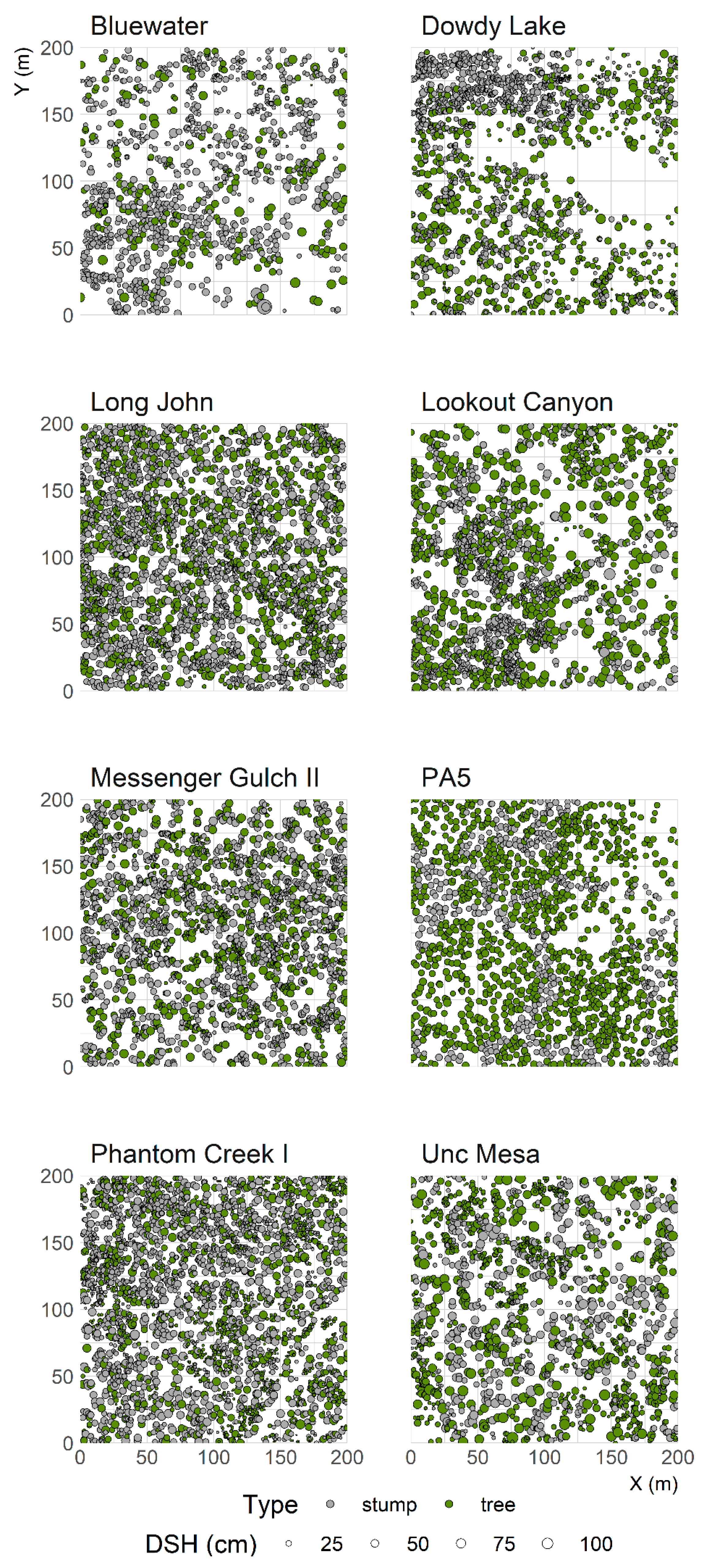
Stem-Maps of Forest Restoration Cuttings in Pinus ponderosa-Dominated Forests in the Interior West, USA


Abstract
:
1. Summary
2. Data Description
3. Methods
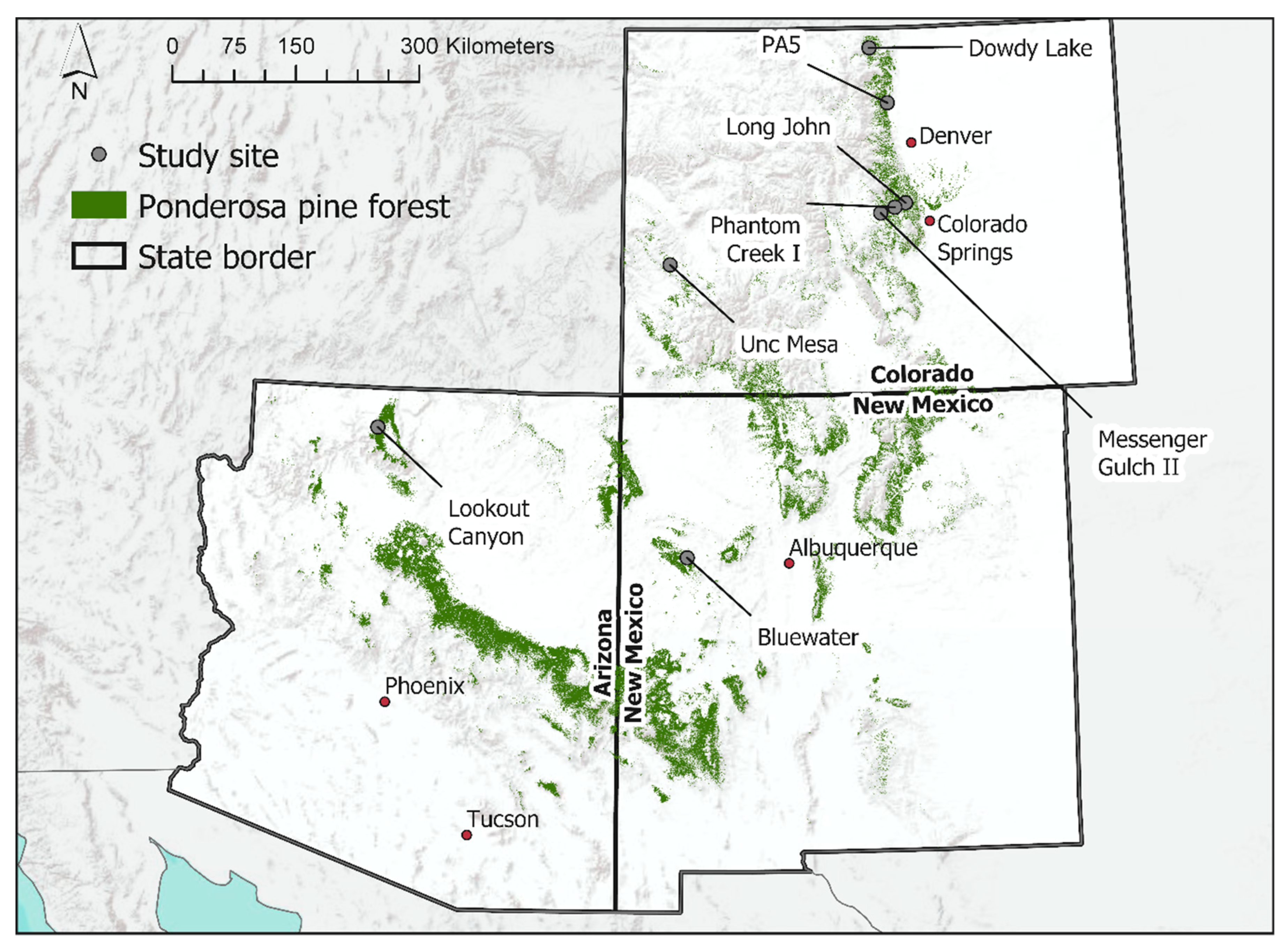
- Cover type: Ponderosa pine forest is dominant.
- Topography: An average slope of less than 5% and few topographic features such as ridges or outcroppings.
- Representativeness: Cuttings should reflect the practices of restoration silviculture implementation at the time.
- Recency: Cuttings should have been implemented in the last decade, to limit observing post-cutting tree recruitment.
Supplementary Materials
Author Contributions
Funding
Acknowledgments
Conflicts of Interest
References
- Watt, A.S. Pattern and process in the plant community. J. Ecol. 1947, 35, 1. [Google Scholar] [CrossRef]
- Pearson, G.A. The role of aspen in the reforestation of mountain burns in Arizona and New Mexico. Plant World 1914, 17, 249–260. [Google Scholar]
- Velázquez, E.; Martínez, I.; Getzin, S.; Moloney, K.A.; Wiegand, T. An evaluation of the state of spatial point pattern analysis in ecology. Ecography. 2016, 39, 1042–1055. [Google Scholar] [CrossRef]
- Levin, S.A. The problem of pattern and scale in ecology. Ecology 1992, 73, 1943–1967. [Google Scholar] [CrossRef]
- Fahey, R.T.; Alveshere, B.C.; Burton, J.I.; D’Amato, A.W.; Dickinson, Y.L.; Keeton, W.S.; Kern, C.C.; Larson, A.J.; Palik, B.J.; Puettmann, K.J.; et al. Shifting conceptions of complexity in forest management and silviculture. For. Ecol. Manag. 2018, 421, 59–71. [Google Scholar] [CrossRef]
- Larson, A.J.; Churchill, D. Tree spatial patterns in fire-frequent forests of western North America, including mechanisms of pattern formation and implications for designing fuel reduction and restoration treatments. For. Ecol. Manag. 2012, 267, 74–92. [Google Scholar] [CrossRef]
- Fulé, P.Z.; Korb, J.E.; Wu, R. Changes in forest structure of a mixed conifer forest, southwestern Colorado, USA. For. Ecol. Manag. 2009, 258, 1200–1210. [Google Scholar] [CrossRef]
- Ziegler, J.; Hoffman, C.; Battaglia, M.; Mell, W. Spatially explicit measurements of forest structure and fire behavior following restoration treatments in dry forests. For. Ecol. Manag. 2017, 386, 1–12. [Google Scholar] [CrossRef]
- Reynolds, R.T.; Meador, A.J.S.; Youtz, J.A.; Nicolet, T.; Matonis, M.S.; Jackson, P.L.; DeLorenzo, D.G.; Graves, A.D. Restoring composition and structure in Southwestern frequent-fire forests: A science-based framework for improving ecosystem resiliency. USDA For. Serv. 2013, RMRS-GTR-310, 76. [Google Scholar]
- Addington, R.N.; Aplet, G.H.; Battaglia, M.A.; Briggs, J.S.; Brown, P.M.; Cheng, A.S.; Dickinson, Y.; Feinstein, J.A.; Pelz, K.A.; Regan, C.M.; et al. Principles and practices for the restoration of ponderosa pine and dry mixed-conifer forests of the Colorado Front Range. USDA For. Serv. 2018, RMRS GTR-3, 121. [Google Scholar]
- Hoffman, C.; Sieg, C.; Linn, R.; Mell, W.; Parsons, R.; Ziegler, J.; Hiers, J. Advancing the science of wildland fire dynamics using process-based models. Fire 2018, 1, 32. [Google Scholar] [CrossRef]
- Parsons, R.; Linn, R.; Pimont, F.; Hoffman, C.; Sauer, J.; Winterkamp, J.; Sieg, C.; Jolly, W. Numerical investigation of aggregated fuel spatial pattern impacts on fire behavior. Land 2017, 6, 43. [Google Scholar] [CrossRef]
- Lutz, J.; Larson, A.; Swanson, M. Advancing fire science with large forest plots and a long-term multidisciplinary approach. Fire 2018, 1, 5. [Google Scholar] [CrossRef]
- Hoffman, C.M.; Canfield, J.; Linn, R.R.; Mell, W.; Sieg, C.H.; Pimont, F.; Ziegler, J. Evaluating crown fire rate of spread predictions from physics-based models. Fire Technol. 2016, 52, 221–237. [Google Scholar] [CrossRef]
- Tinkham, W.T.; Dickinson, Y.; Hoffman, C.M.; Battaglia, M.A.; Ex, S.; Underhill, J. Visualization of heterogeneous forest structures following treatment in the Southern Rocky Mountains. USDA For. Serv. 2017, RMRS-GTR-3, 72. [Google Scholar]
- Matonis, M.S.; Binkley, D. Not just about the trees: Key role of mosaic-meadows in restoration of ponderosa pine ecosystems. For. Ecol. Manag. 2018, 411, 120–131. [Google Scholar] [CrossRef]
- Ziegler, J.P.; Hoffman, C.M.; Fornwalt, P.J.; Sieg, C.H.; Battaglia, M.A.; Chambers, M.E.; Iniguez, J.M. Tree regeneration spatial patterns in ponderosa pine forests following stand-replacing fire: Influence of topography and neighbors. Forests 2017, 8, 391. [Google Scholar] [CrossRef]
- Churchill, D.J.; Larson, A.J.; Dahlgreen, M.C.; Franklin, J.F.; Hessburg, P.F.; Lutz, J.A. Restoring forest resilience: From reference spatial patterns to silvicultural prescriptions and monitoring. For. Ecol. Manag. 2013, 291, 442–457. [Google Scholar] [CrossRef]
- Bettinger, P.; Tang, M. Tree-level harvest optimization for structure-based forest management based on the species mingling index. Forests 2015, 6, 1121–1144. [Google Scholar] [CrossRef]
- Maher, C.T.; Oja, E.; Marshall, A.; Cunningham, M.; Townsend, L.; Worley-Hood, G.; Robinson, L.R.; Margot, T.; Lyons, D.; Fety, S.; et al. Real-time monitoring with a tablet app improves implementation of treatments to enhance forest structural diversity. J. For. 2019, 117, 280–292. [Google Scholar] [CrossRef]
- Toney, C.; Reeves, M. Equations to convert compacted crown ratio to uncompacted crown ratio for trees in the interior West. West. J. Appl. For. 2009, 24, 76–82. [Google Scholar]


| Variable | Description |
|---|---|
| type * | Either tree or stump |
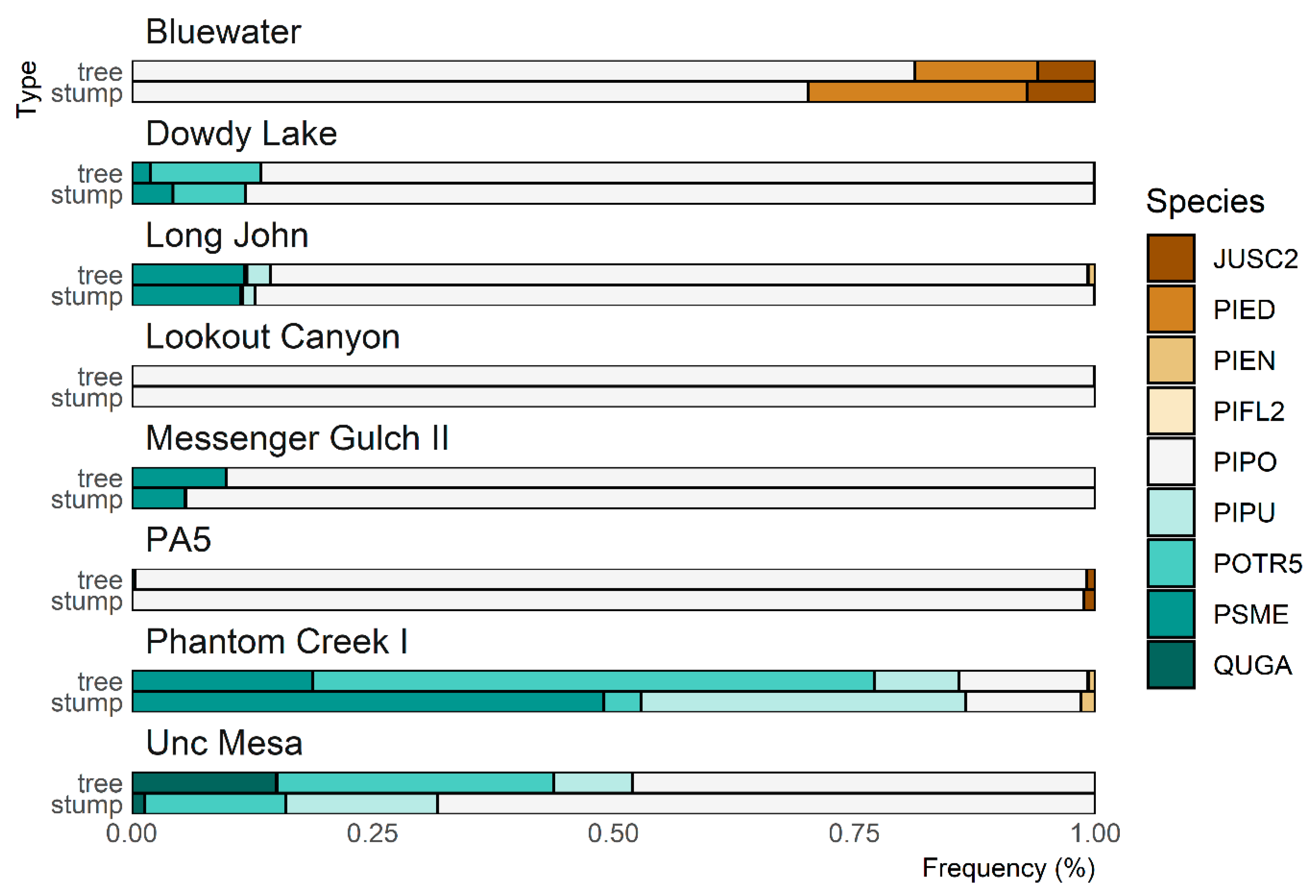
| species | four-letter code for tree species name (PLANTS Database; http://plants.usda.gov) |
| dbh | Diameter at breast height; tree bole diameter at 1.37 m above the ground |
| dsh | Diameter at stump height; tree bole diameter at 15 cm above the ground |
| ht | Tree height (m) |
| cbh | Crown base height (m); compacted crown base height (Toney and Reeves, 2009) |
| cw | Crown width (m); average width of tree crown |
| x | Coordinate in the x dimension |
| y | Coordinate in the y dimension |
| Type/Variable | Site | |||||||
|---|---|---|---|---|---|---|---|---|
| Bluewater | Dowdy Lake | Long John | Lookout Canyon | Messenger Gulch II | PA5 | Phantom Creek I | Unc Mesa | |
| Stump | ||||||||
| Mean dsh (cm) | 20.77 | 16.37 | 20.29 | 19.53 | 22.02 | 25.60 | 19.17 | 28.43 |
| n | 1055 | 1331 | 2248 | 1137 | 1663 | 495 | 2308 | 759 |
| Tree | ||||||||
| Mean dbh (cm) | 30.39 | 21.45 | 22.22 | 30.91 | 17.54 | 24.00 | 12.77 | 19.59 |
| Mean dsh (cm) | 36.46 | 26.80 | 28.32 | 40.75 | 23.11 | 29.32 | 16.02 | 23.02 |
| Mean height (m) | 12.63 | 8.82 | 12.72 | 15.93 | 8.67 | 7.97 | 7.55 | 9.69 |
| Mean cbh (m) | 4.56 | 3.4 | 5.23 | 6.69 | 3.58 | 3.70 | 3.53 | 4.28 |
| Mean crown width (m) | 4.04 | 3.35 | 3.60 | 4.35 | 2.81 | 3.70 | 2.51 | 3.13 |
| n | 251 | 725 | 1071 | 812 | 1077 | 1177 | 1429 | 1247 |
© 2019 by the authors. Licensee MDPI, Basel, Switzerland. This article is an open access article distributed under the terms and conditions of the Creative Commons Attribution (CC BY) license (http://creativecommons.org/licenses/by/4.0/).
Share and Cite
Ziegler, J.P.; Hoffman, C.M.; Battaglia, M.A.; Mell, W. Stem-Maps of Forest Restoration Cuttings in Pinus ponderosa-Dominated Forests in the Interior West, USA. Data 2019, 4, 68. https://doi.org/10.3390/data4020068
Ziegler JP, Hoffman CM, Battaglia MA, Mell W. Stem-Maps of Forest Restoration Cuttings in Pinus ponderosa-Dominated Forests in the Interior West, USA. Data. 2019; 4(2):68. https://doi.org/10.3390/data4020068
Chicago/Turabian StyleZiegler, Justin P., Chad M. Hoffman, Mike A. Battaglia, and William Mell. 2019. "Stem-Maps of Forest Restoration Cuttings in Pinus ponderosa-Dominated Forests in the Interior West, USA" Data 4, no. 2: 68. https://doi.org/10.3390/data4020068
APA StyleZiegler, J. P., Hoffman, C. M., Battaglia, M. A., & Mell, W. (2019). Stem-Maps of Forest Restoration Cuttings in Pinus ponderosa-Dominated Forests in the Interior West, USA. Data, 4(2), 68. https://doi.org/10.3390/data4020068