Predictive Models of Student College Commitment Decisions Using Machine Learning

Abstract

Every year, academic institutions invest considerable effort and substantial resources to influence, predict and understand the decision-making choices of applicants who have been offered admission. In this study, we applied several supervised machine learning techniques to four years of data on 11,001 students, each with 35 associated features, admitted to a small liberal arts college in California to predict student college commitment decisions. By treating the question of whether a student offered admission will accept it as a binary classification problem, we implemented a number of different classifiers and then evaluated the performance of these algorithms using the metrics of accuracy, precision, recall, F-measure and area under the receiver operator curve. The results from this study indicate that the logistic regression classifier performed best in modeling the student college commitment decision problem, i.e., predicting whether a student will accept an admission offer, with an AUC score of 79.6%. The significance of this research is that it demonstrates that many institutions could use machine learning algorithms to improve the accuracy of their estimates of entering class sizes, thus allowing more optimal allocation of resources and better control over net tuition revenue.

1. Introduction

The future and sustainability of the traditional higher education business model [1] is an important topic of discussion. These issues are of course highly dependent on the type of academic institution being considered, such as public colleges and universities, private non-profit colleges and private for-profit colleges. Incoming students face multiple financial pressures: rising tuition costs, concerns about incurred debt, unsure post-graduation job prospects and the availability of cheaper alternatives such as massive open online courses (MOOCs) [2] and other online options. The economic pressures felt by incoming students surely impacts their willingness to make the large financial commitments required to enroll in many colleges and universities. To alleviate monetary stresses caused by fluctuations in student enrollment, institutions of higher education often try to operate at full capacity, which means increasing, or at the very least optimizing, their tuition income. Our research was motivated by a desire to accurately predict incoming student class size and therefore tuition-based income.

The published cost of attending a nationally ranked liberal arts college such as Occidental College [3] is $70,182 for the 2018–2019 academic year [4]. If the college falls below its target enrollment by as few as 10 students (which in the case of Occidental College would be less than 2% of the expected annual entering student enrollment of 550), this could result in a potential financial loss of $701,820 per year for four years, amounting to a total estimated loss of more than $2.8 million. (The reader should note that this estimate only represents the maximum potential financial loss due to an enrollment shortfall of 10 students and that most students attending an institution such as Occidental College effectively receive a discounted price due to financial aid [5].) It is very important for an academic institution to know fairly accurately how many incoming students they can expect to enroll each year, especially if they are dependent on the revenue generated by students [6]. The research presented in this paper can be used by these institutions to achieve this by predicting which students are more likely to accept admission offers.

The model we develop in this paper has broad significance, wide applicability and easy replicability. We address an important question facing almost every institution of higher education: “Which admitted students will actually accept their admission offers?” Being able to accurately predict whether a student admitted to an academic institution will accept or reject their admissions offer can help institutions of higher education manage their student enrollments. For many institutions, enrollment management is an extremely important component of academic administration [7]. The data required to develop our model are readily available to most institutions as a part of the admissions process, which makes the research presented here widely applicable and easily replicated.

The goal of our research is to develop a model that can make an accurate prediction regarding each student’s college commitment decision by classifying the student into one of two categories: accepts admission offer and rejects admission offer. In other words, we characterize the student college commitment decision problem as a binary classification problem [8] using supervised machine learning [9,10]. We want to be able to classify new instances, i.e., when presented with a new admitted student we would like our model to correctly predict whether that student will accept or reject the admission offer. We use the term “model” [8,9,10] to refer to the specific algorithm we select after implementing multiple machine learning techniques on our training data. We view the classification problem we are working on as a supervised machine learning problem. Supervised machine learning problems are a class of problems which can generalize and learn from labeled training data, i.e., a set of data where the correct classification is known [11,12,13]. From 2014 to 2017, Occidental College received an average of 6292 applications per year, with admission offered to approximately 44% of these applicants, or 2768 students, of which 19.5% or 535 students actually enrolled [14]. (This whittling process is depicted visually in Figure 1.) Using four years of detailed data provided by the college, we are able to characterize and classify every student in the admitted pool of students.

The rest of this paper is organized as follows. In Section 2, we provide a literature review of the work that has been conducted on the applications of machine learning techniques in the context of educational settings. We divide Section 3, our discussion of Materials and Methods, into two parts. In Section 3.1, we provide details about the data, discuss the preprocessing steps required to clean the raw dataset to make it suitable to be used in a machine learning algorithm, and explore the data. Next, in Section 3.2, we describe the implementation steps, define multiple success metrics used to address class imbalance in our data and then discuss feature selection. We present the results of our predictions using various metrics of success in Section 4. Lastly, we summarize our results, mention other possible techniques and provide avenues for future research in Section 5. In Appendix A, we provide brief descriptions of the seven machine learning methods used in the research presented here.

2. Literature Review

There are many examples of the application of machine learning techniques to analyze data and other information in the context of educational settings. This area of study is generally known as “educational data mining” (EDM) and it is a recently emergent field with its own journals [15], conferences [16] and research community [17,18]. A subset of EDM research that focuses on analyzing data in order to allow institutions of higher education better clarity and predictability on the size of their student bodies is often known as enrollment management. Enrollment management is “an organizational concept and systematic set of activities whose purpose is to exert influence over student enrollment” [7].

Below, we provide multiple examples of research by others that combines aspects of enrollment management with applications of data science techniques in various educational settings. These are applications of machine learning to: college admission from the student perspective; supporting the work of a graduate admission committee at a PhD granting institution; predicting student graduation time and dropout; monitoring student progress and performance; evaluating effectiveness of teaching methods by mining non-experimental data of student scores in learning activities; and classifying the acceptance decisions of admitted students.

There are many websites which purport to predict college admission from the perspective of an aspiring student. A few examples are go4ivy.com1, collegeai.com2, project.chanceme3, and niche.com4. Websites such as these claim to utilize artificial intelligence to predict a student’s likelihood of being admitted to a college of their choice without providing specific details about software used and techniques implemented. Our work differs in that we are predicting the likelihood of a student accepting an admission offer from a college not providing an estimate of the chances of a student’s admission to college. Unlike these websites, we provide a complete description of our materials and methods below.

In the work of Waters and Miikkulainen [19], machine learning algorithms were used to predict how likely an admission committee is to admit each of 588 PhD applicants based on the information provided in their application file. Students whose likelihood of admission is high have their files fully reviewed to verify the model’s predictions and increase the efficiency of the admissions process by reducing the time spent on applications that are unlikely to be successful. Our research differs from this work in multiple ways; our setting is at the undergraduate level, we classify decisions by the students not decisions by the college; our dataset is an order of magnitude larger; and the feature being optimized is incoming class size not time spent on decision making.

Yukselturk et al. [20] discussed using data mining methods to predict student dropout in an online program of study. They used surveys to collect data from 189 students and, after analysis, identified the most important features in predicting which students will complete their online program of study. The only similarity between this work and ours is that it is an application of machine learning in an educational setting. The data used for our analysis are not survey data; we are attempting to predict whether a student will accept a college admission offer, not whether a student drops out of an online program of study and the size of our dataset is an order of magnitude larger.

There are multiple authors who use data science techniques to describe and predict student progress and performance in educational settings. Tampakas et al. [21] analyzed data from about 288 students and applied machine learning algorithms to classify students into one of two categories “Graduate” or “Fail”. They then predicted which of the graduating students would take four, five or six years to graduate. While this research, similar to ours, can be classified as educational data mining, the focus and goals are very different. Our work is about predicting student college commitment decisions, while their work is about modeling student academic behaviour in college. Using data from 2260 students, Livieris et al. [22,23] were able to predict with high accuracy which students are at risk of failing and classified the passing students as “Good”, “Very Good” and “Excellent”. The authors developed a decision support software program (available at https://thalis.math.upatras.gr/~livieris/EducationalTool/) that implements their work and made it freely available for public use. Our research presented below differs in that we are not trying to monitor or categorize student progress and performance in school. Instead, our work tries to predict student college commitment decisions using multiple machine learning techniques.

Duzhin and Gustafsson [24] used machine learning to control the effect of confounding variables in “quasi-experiments” that seek to determine which teaching methods have the greatest effect on student learning. The authors considered teaching methods such as clickers, handwritten homework and online homework with immediate feedback and included the confounding variables of student prior knowledge and various student characteristics such as diligence, talent and motivation. Our work differs in that it tries to predict student college commitment decisions using multiple machine learning techniques and its potential benefit is to the school’s finances, while the work in [24] seeks to assist instructors in identifying teaching methods that work best for them.

The research presented in our paper and in Chang’s paper [25] both use educational data mining to predict the percentage of admitted students who ultimately enroll at a particular college. This ratio is known as the yield rate and it varies widely among different institutions [26]. While the central goal of modeling yield rate is common to both works, there are also significant differences. Some of these are the institutional setting, the number of algorithms applied and how characteristics of the data are addressed. Our work is set at a small, liberal arts college of approximately 2000 students, while Chang’s is set at a large public university. We utilize seven machine learning techniques while Chang used three. Our work and Chang’s also differ in how we address the challenges that arise from characteristics of the dataset.

We acknowledge that the specific educational context in which we apply several machine learning algorithms to the analysis of “big data” obtained from the college admission process appears to be relatively unexplored in the literature. However, we believe our work demonstrates this is a fruitful area of research.

3. Materials and Methods

In this section, we provide numerous details about the data, discuss the preprocessing of the data, perform data exploration, and summarize our methodology [8,9,10]. This includes both a flowchart visualization (in Figure 2) and a narrative summary (in Section 3.2.1), of the materials and methods used. Next, we define several success metrics to measure model performance and identify which ones are appropriate to use with our data. Finally, we describe our feature selection process.

We explored and compared several supervised machine learning classification techniques to develop a model which accurately predicts whether a student who has been admitted to a college will accept that offer. The machine learning techniques utilized are:

• Logistic Regression (LG)
• Naive Bayes (NB)
• Decision Trees (DT)
• Support Vector Machine (SVM)
• K-Nearest Neighbors (K-NN)
• Random Forests (RF)
• Gradient Boosting (GB)

One of the motivations for the research presented in this paper is a desire to demonstrate the utility of the application of well-known machine learning algorithms to our specific problem in educational data mining. The above supervised machine learning techniques constitute some of the most efficient and frequently utilized algorithms [27].

3.1. Data

Here, we describe and discuss the data we used in our student college commitment decision problem. Our dataset was obtained from the Occidental College Admissions Aid Office [14]. The dataset covers admissions from 2014 to 2017 and consists of $11,001$ admitted applicants (observations) along with 35 pieces of personal information associated with each student (variables). There are twelve numerical variables present such as “GPA” (grade point average) and “HS Class Size” (high school class size), with the remaining variables being categorical and binary in nature such as “Scholarship” and “Gender”, respectively. Note that “SAT I Critical Reading”, “SAT I Math”, “SAT I Writing”, “SAT I Superscore”, “SATR”, “SATR EBRW”, “SATR Math”, “SATR Total’ and “ACT Composite Score” are various examples of scores associated with standardized tests taken by students interested in applying to college. (SAT is “Scholastic Assessment Test’ and ACT is “American College Test”.) Students pay to take these exams and then also pay to have their scores transmitted to colleges to which they are applying. The list of all 35 variables with their variable type can be found in

Table 1. List of variables.

Binary	Categorical	Numerical
Gross Commit Indicator	Application Term	GPA
Net Commit Indicator	Ethnic Background	HS Class Rank
Final Decision	Permanent State/Region	HS Class Size
Financial Aid Intent	Permanent Zip Code/Postal Code	ACT Composite Score
Gender	Permanent Country	SAT I Critical Reading
Legacy	Current/Most Recent School Geomarket	SAT I Math
Direct Legacy	First Source Date	SAT I Writing
First Generation Indicator	First Source Summary	SAT I Superscore
Campus Visit Indicator	Top Academic Interest	SATR EBRW
Interview	Extracurricular Interests	SATR Math
Recruited Athlete Indicator	Level of Financial Need	SATR Total
	Scholarship	Reader Academic Rating

. The target variable, i.e., the variable we wish to predict, “Gross Commit Indicator”, is in bold. Note the variables are organized into columns corresponding to type, i.e., binary, categorical and numerical.

Figure 1 is a flowchart that visually represents the admission whittling process for the classes of 2018 to 2021 (students admitted in 2014 to 2017). The total number of applicants in these four years was $25,166$. Among them, $11,001$ were admitted and 2138 students accepted their admission offers.

We use the term “admits” to represent students whom the college has extended an admission offer to, “commits” to represent the students who have accepted the offer and “uncommits” for students who decline or reject the admission offer. Note that international students and early decision students have been omitted from our dataset and this reduced our dataset from 11,001 to 9626 admits.

In

Table 2. Counts and percentages of first-year commit data (raw).

Application Year	Class of 2018	Class of 2019	Class of 2020	Class of 2021	Total
Applicants	6071	5911	6409	6775	25,166
Admits	2549	2659	2948	2845	11,001
Admit Percentage	42%	45%	46%	42%	44%
Commits	547	518	502	571	2138
Commit Percentage	21%	19%	17%	20%	19%
Uncommits	2002	2141	2446	2274	8863
Uncommit Percentage	79%	81%	83%	80%	81%

, we present counts of the applicants, admits, commits and uncommits by year for the last four years starting from 2014 (Class of 2018) to 2017 (Class of 2021).

In Table 2, we also present admit percentage (fraction of applicants who become admits) and commit percentage (fraction of admits who become commits) for the last four years starting from 2014 (Class of 2018) to 2017 (Class of 2021). Our use of “commit percentage” is equivalent to what other authors refer to as the yield or yield rate [26].

Each admitted applicant can be viewed as belonging to one of two categories: accepts admission offer (commit) or rejects admission offer (uncommit). Over the four years of data that we used for our study, only 19.5% of all students fall into the commit category and 80.5% of students fall in the uncommit category. Note the ratio of uncommits to commits is approximately 4:1, which means that there is an imbalance in the data for our binary classification problem. Generally, for a supervised machine learning algorithm to be successful as a classifier, one wants the classes to be roughly equal in size. The consequences of this “class imbalance” [28] is discussed in Section 3.2. Below, we discuss the steps used to cleanse the raw data received from Occidental College so that it can be used in the seven machine learning algorithms we decided to use. Then, we analyzed the data to help us better understand the relationships the variables share with the purpose of being able to identify which among the 34 features have the most power to predict the target variable “Gross Commit Indicator”.

3.1.1. Preprocessing

Preprocessing is an important step in any data science project; the aim is to cleanse the dataset and prepare it to be further used in a prediction algorithm. The data received from Occidental College had few missing entries and thus we only needed to make a few changes to make the data suitable for our chosen machine learning algorithms.

A standard challenge in data cleaning is determining how to deal with missing data. It is important to identify the features with missing entries, locate such entries and implement a treatment based on the variable type that allows us to use the data in the model, since the feature in question may be a strong predictor in determining the algorithms outcome.

Numerical variables required two different treatments: normalization and data imputation. Numerical variables where there are no missing entries such as “Reader Academic Rating” were rescaled to a unitary range. For numerical variables with missing entries such as “GPA”, the median of the available entries was computed and used to replace the missing entries. This process is called data imputation [8].

Categorical variables required special treatment to prepare them for input into the machine learning algorithms. Entries that had missing categorical features (“Gender”, “Ethnic Background”, etc.) were dropped from the dataset. All categorical variables were processed using one-hot encoding [8]. One-hot encoding is a method in which categorical variables are represented as binary vectors with a label for which class the data belongs to by assigning 0 to all the dimensions and 1 for the class the data belongs to. For example, the categorical variable “Level of Financial Need” has three possible classes: High, Medium, and Low. One-hot encoding transforms a student with high level of financial need into the vector $[1,0,0]$, a student with medium level of financial need into the vector $[0,1,0]$ and an applicant with low level of financial need as $[0,0,1]$.

After the pre-processing of the dataset was completed, the number of admits was 7976 with 1345 commits and 6631 uncommits. We have made the original dataset of 9626 admits publicly available (https://github.com/kbasu2016/Occidental-College-Acceptance-Problem/).

3.1.2. Data Exploration

We explored the data to garner intuition and make observations regarding patterns and trends in the data.

Table 3. Significance of GPA.

GPA Bin	Accept Percentage	Reject Percentage	Number of Students
$2.0+$	100	0	1
$2.2+$	33	67	3
$2.4+$	100	0	4
$2.6+$	43	57	14
$2.8+$	53	47	34
$3.0+$	71	29	152
$3.2+$	77	23	586
$3.4+$	79	21	1424
$3.6+$	85	15	2577
$3.8+$	87	13	3324
$4.0$	89	11	1412

illustrates the significance of “GPA” as a variable in predicting student college commitment decisions and indicates that the percentage of commits co-varies with the grade point average (GPA).

Table 4. Significance of campus visit.

	Accept Percentage	Reject Percentage	Number of Students
Visited Campus	23	77	5122
Didn’t Visit Campus	7	93	4409

illustrates the effect of the campus visit on student college commitment decisions. From the Occidental College Admission Office, we learned that they believe that whether an admitted student visited the campus prior to accepting the admissions offer plays an important role in determining student acceptance. The table clearly indicates a greater proportion of students who visit the campus accept the admission offer (23% versus 7%). This is significant because it reaffirms the Admissions Office belief that students who participate in campus visits are more likely to accept admission offers.

3.1.3. Prediction Techniques

To achieve the goal of predicting student college commitment decisions, we compared the performance of several binary classification techniques and selected the best one. Our target variable (the variable we wish to predict: “Gross Commit Indicator”) takes on the value 1 if the admitted applicant accepts the offer, and 0 if the admitted applicant rejects the offer. Seven binary classifiers were implemented to predict this target variable and we provide a brief explanation of each method in Appendix A.

3.2. Methodology

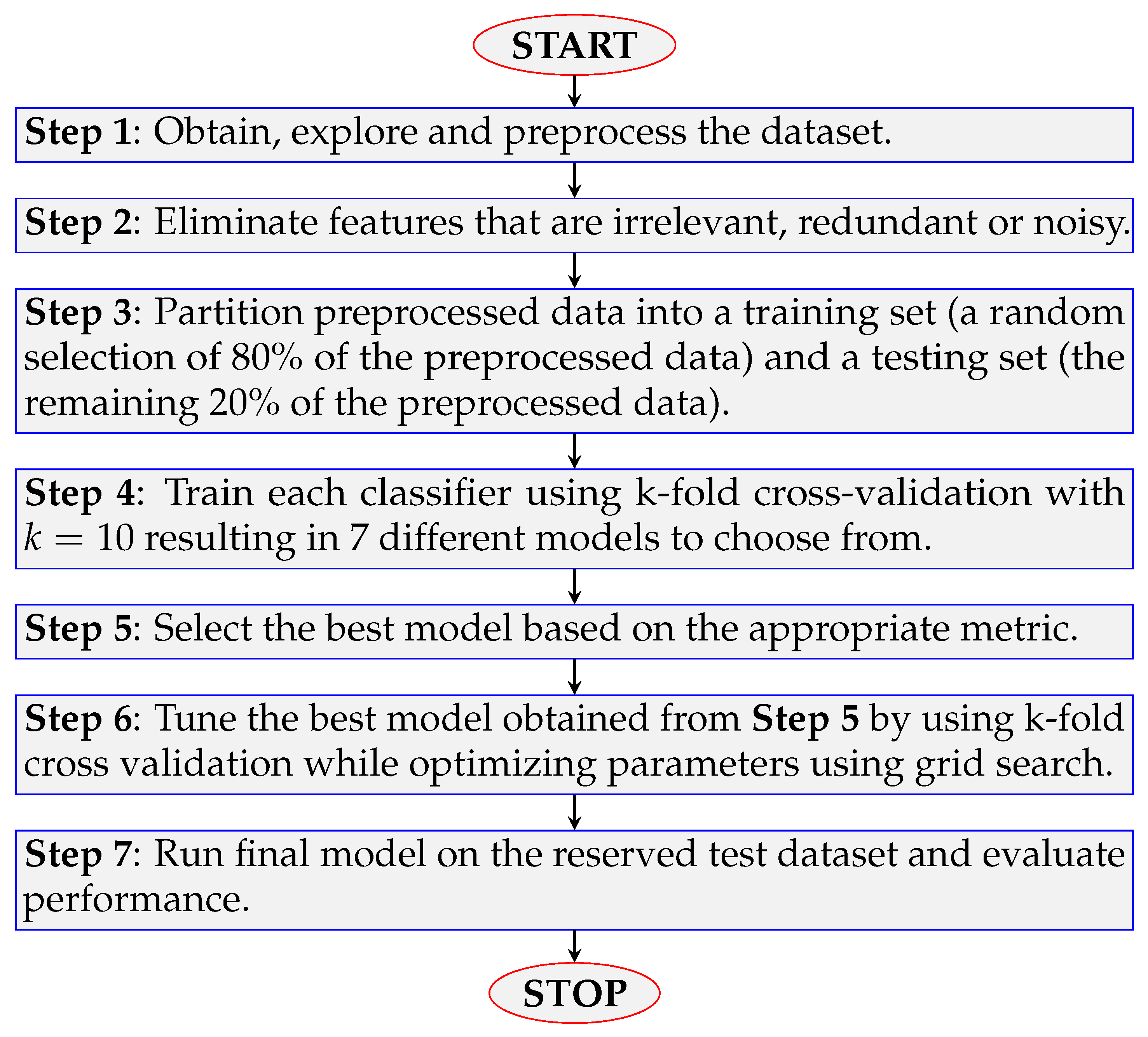
Here, we discuss the methodology used to produce our predictive model of student college commitment decisions. The steps implemented to identify the final optimized model are illustrated in a flow chart given in Figure 2.

3.2.1. Implementation

Below, we provide a short narrative summary of the steps shown in Figure 2 to develop our model of college student commitment decisions. The data were pre-processed and randomly separated into a training set and a testing set. We chose our training set to be 80% of the 7976 entries in our dataset.

Before the training data were used to train each selected machine learning algorithm, we identified a subset of features that have the most power in predicting the target variable “Gross Commit Indicator”. This process of pruning irrelevant, redundant and noisy data is known as feature selection or dimensionality reduction [29] and is discussed in detail in Section 3.2.3. Selecting relevant features for input into a machine learning algorithm is important and can potentially improve the accuracy and time efficiency of the model [8,10].

Next, we applied the k-fold cross validation technique with $k=10$ on the training data. k-fold cross validation is a model validation technique for assessing how the results of a machine learning algorithm will generalize to an unseen dataset [30]. The k-fold cross validation splits the training data into k equal sub-buckets. Each algorithm is then trained using $(k-1)$ sub-buckets of training data, and the remaining kth bucket is used to validate the model by computing an accuracy metric. We repeated this process k times, using all possible combinations of $(k-1)$ sub-buckets and one bucket for validation. We then averaged out the accuracy metric of all the k different trial runs on each model.

The k-fold cross-validation process may limit problems like under-fitting and over-fitting [10]. Under-fitting occurs when the model has large error on both the training and testing sets. Over-fitting occurs when the model has little error on the training set but high error on the testing set.

The model with the highest AUC score (see definition 4 below) on the training data was then selected as the “best model” from amongst the selected classifiers [31]. That model’s performance on the training set was optimized by parameter selection and evaluated on the unseen testing dataset. The optimized algorithm produced reasonable results on the testing set.

3.2.2. Resolution of Class Imbalance: Different Success Metrics

Here, we present the resolution of the inherent class imbalance of our dataset that we first observed and discussed in Section 3.1. Most binary classification machine learning algorithms work best when the number of instances of each class is roughly equal. When the number of instances of one class far exceeds the other, problems arise [29].

In the case of the Occidental College admissions dataset, one can observe in Table 2 that on average only 19.5% of all students offered admission accept the offer extended by the college. In other words, 80.5% of all admitted students in this dataset reject the admission offer. This is an example of class imbalance in a dataset. In this situation, if a putative classification algorithm were to always predict that a new student will reject the admission offer, the algorithm would be correct 80.5% of the time. This would be considered highly successful for most machine learning algorithms, but in this case is merely a result of the class imbalance. We resolve this issue by analyzing the performance of our machine learning algorithms using multiple measures in addition to accuracy such as precision, recall, F-measure, and AUC or ROC score.

Given a set of labeled data and a predictive model, every prediction made will be in one of the four categories:

• True positive: The admitted student accepted the offer and the model correctly predicted that the student accepted the offer (correct classification).
• True negative: The admitted student rejected the offer and the model correctly predicted that the student would reject the offer (correct classification).
• False positive (Type I Error): The admitted student rejected the offer, but the model incorrectly predicted the student would accept the offer (incorrect classification).
• False negative (Type II Error): The admitted student accepted the offer, but the model incorrectly predicted that the student would reject the offer (incorrect classification).

These categories can also be represented in a confusion matrix [10], as depicted in

Table 5. Confusion matrix.

	Predicted Accept	Predicted Reject
Accepted	True Positive	False Negative
Rejected	False Positive	True Negative

, that allows us to visualize the performance of a supervised machine learning algorithm. A perfect predictive model would have only true positives and true negatives, thus its confusion matrix would have nonzero values only on its main diagonal. While a confusion matrix provides valuable information about a model’s performance, it is often preferred to have a single metric to easily compare the performance of multiple classifiers [8].

Accuracy is usually the first measure used to determine whether a machine learning algorithm is making enough correct predictions. Using accuracy as a metric to evaluate the performance of a classifier can often be misleading, especially in the case of class imbalance [28].

Simply using the accuracy score could result in a false impression regarding the model performance, since only 19.5% of all admits accept the admission offer, which indicates class imbalance is present in our dataset. Instead, we used the more suitable metrics of precision, recall, $F_{\beta }$ score and area under the receiver operator curve to overcome the challenges caused by this class imbalance [9]. Below, we provide the definition of the standard performance evaluation metric of accuracy, and also include definitions of more appropriate measures of performance when class imbalance is present.

Definition 1.

Accuracy

Accuracy measures how often the classifier makes the correct prediction. In other words, it is the ratio of the number of correct predictions to the total number of predictions. Accuracy is defined as the fraction of correct predictions.

$$\mathit{accuracy}=\frac{\mathit{true}\mathit{positive}+\mathit{true}\mathit{negative}}{\mathit{true}\mathit{positive}+\mathit{false}\mathit{positive}+\mathit{false}\mathit{negative}+\mathit{true}\mathit{negative}}$$

(1)

Definition 2.

$F_{\beta }$ score

The $F_{\beta }$ score is the weighted harmonic mean of precision and recall, reaching its optimal value at 1 and its worst value at 0.

$$F_{\beta }\mathit{score}=(1+{\beta }^2)\times \frac{\mathit{precision}\times \mathit{recall}}{({\beta }^2\times \mathit{precision})+\mathit{recall}}$$

(2)

The β parameter determines the weight of precision in the combined score, i.e, $\beta <1$ lends more weight to precision, and $\beta >1$ favors recall. When $\beta =1$ the resulting $F_1$ score is the harmonic mean of precision and recall and thus must lie between them [8]. Further, $\beta =0$ considers only precision and $\beta \to \infty$ considers only recall.

Definition 3.

ROC

The receiver operating characteristic (ROC) curve is another commonly used summary for assessing the diagnostic ability of a binary classifier over all possible results as its class discrimination threshold is varied [8,30]. Class discrimination is most often set to be $0.5$. The ROC curve is a plot of the true-positive rate (also known as sensitivity or recall) versus the false-positive rate.

Definition 4.

AUC Score

The AUC score is defined as the area under the ROC curve. The AUC score measures the overall performance of a classifier without having to take into consideration the class distribution or misclassification cost. The closer the AUC score (the area under the ROC curve) is to 1 (the maximum possible value), the better the overall performance of the binary classifier.

In the student college commitment decision problem, we prefer a model with high precision (i.e., one that is more likely to correctly predict which students will actually accept admission offers). It would be more harmful to the college if the algorithm incorrectly predicts a student will accept the admission offer when in reality they reject it, compared to the tradeoff of having a student accept the offer unexpectedly. Since our model requires high precision, we use the $F_{0.5}$ score to evaluate model performance, so that precision is more heavily weighted than recall. Figure 3 illustrates visually the rationale for our selection of the $F_{0.5}$ score as our chosen success metric.

We decided to use a metric to evaluate and compare classifiers and another metric to identify the optimal one. We used the AUC scores to evaluate and compare the seven selected classifiers and choose the best performing algorithm with respect to this metric. We then used the $F_{0.5}$ score to confirm our optimal selection. These results are presented in Section 4.

3.2.3. Feature Selection

The inclusion of irrelevant, redundant and noisy data can negatively impact a model’s performance and prevent us from identifying any useful and noteworthy patterns. Additionally, incorporating all existing features in a model is computationally expensive and leads to increased training time [8,10,29]. Thus, we focused on reducing the 34 available features (note that “Gross Commit Indicator” is the target variable) for the Occidental College admissions dataset given in Table 1, a process known as feature selection or dimensionality reduction.

There were various reasons for the elimination of certain variables from consideration in the model. For example, most variables that contain geographic location information such as “Permanent Postal”, “Permanent Country” and “School Geomarket” were not used with any of the machine learning classifiers. Due to the complexity of its implementation, we decided to postpone incorporating geographic features in this model. Features that are logically irrelevant to the admission decision making process of an applicant such as “Application Term”, “Net Commit Indicator”, etc. were also dropped. In the case of redundant categorical variables such as “Legacy” and “Direct Legacy”, one (“Legacy”) was eliminated.

Next, we eliminated redundant numerical variables. We began by computing the correlation coefficient between all numerical variables. The correlation coefficient r is a numerical measure of the direction and strength of a linear association and is denoted by $r=\frac{\sum z_x{z}_y}{n-1}$ where $(z_x,z_y)=(\frac{x-\overline{x}}{s_x},\frac{y-\overline{y}}{s_y})$. Here, $\overline{x}$ and $s_x$ are the mean and standard deviation respectively of the predictor variable x and similar notations hold for the variable y. The purpose of this process is to ensure that our machine learning algorithms do not incorporate features that are collinear, since collinearity deteriorates model performance [32,33]. If two numerical variables x and y are highly correlated ($\left|r\right|\ge 0.7$), then one of them is dropped. In [34], values of $\left|r\right|>0.5$ are said to indicate strong correlation. The numerical variable that has a higher correlation with the target variable remains in the model.

Table 6. Correlation coefficients of non-collinear numerical variables.

Numerical Variable	GPA	HS Class Size	RAR
GPA	1.0000	0.0045	−0.6100
HS Class Size	0.0045	1.0000	−0.0820
Reader Academic Rating (RAR)	−0.6100	−0.0820	1.0000

displays the three numerical variables (“GPA”, “HS Class Size”, “Reader Academic Rating”) that remain for incorporation into the machine learning algorithms. One can see from the correlation coefficients r in the table that our model does not incorporate any collinear features, i.e., the features are not linearly correlated since their values of $\left|r\right|$ are substantially less than $0.7$.

The goal of feature selection is to determine which features provide the most predictive power and to eliminate those which do not contribute substantially to the performance of the model. The process known as recursive feature elimination (RFE) results in the removal of features such as “Top Academic Interest” and “Recruited Athlete Indicator”. We implemented RFE in Python (Scikit-Learn Feature Selection5) to identify the least important features remaining and removed them from the list of features under consideration found in Table 1 [35].

After completion of feature selection we were able to narrow down the 34 original variables to the 15 variables listed below in

Table 7. Selected features.

Variable Name	Description	Range
Financial Aid Intent	binary	Y/N
Scholarship	categorical	type of scholarship program
Direct Legacy	binary	Y/N
Ethnic Background	categorical	e.g., Hispanic, White
First Generation Indicator	binary	Y/N
Permanent State/Region	categorical	e.g., NY, CA
GPA	numerical	0–4
HS Class Size	numerical	1–5000
Campus Visit Indicator	binary	Y/N
Interview	binary	Y/N
Top Academic Interest	categorical	Politics, Marine Biology
Extracurricular Interests	categorical	e.g., Dance, Yoga
Gender	binary	M/F
Level of Financial Need	categorical	High/Medium/Low
Reader Academic Rating (RAR)	numerical	1–5

with their corresponding type and range.

We use only these 15 features when implementing the pre-selected supervised machine learning algorithms given in Appendix A.

4. Results

4.1. Choosing the Final Model: Classifier Comparison and Hyperparameter Optimization

In this subsection, we discuss the results obtained from applying our selected classifiers on the pre-processsed admissions dataset containing 7976 instances. All supervised machine learning algorithms applied in this study have been developed using the open-source, object-oriented programming language Python 3.0 and its many packages such as scikit-learn [35,36].

Table 8. Performance evaluation of supervised algorithms.

Classifier	CV_Accuracy	Run Time (s)	CV_AUC	Run Time (s)
Logistic Regression	85.53%	48.72	77.79%	47.60
Naive Bayes	85.13%	46.82	66.99%	47.14
Decision Trees	82.59%	199.80	59.47%	199.57
SVM	83.13%	2111.62	66.61%	2112.58
10-Nearest Neighbors	84.78%	856.00	69.45%	857.88
Random Forests	86.18%	245.08	72.85%	242.51
Gradient Boosting	84.96%	10,461.47	76.02%	10,308.31

presents the cross-validated accuracy score and cross-validated AUC scores for all the binary classification algorithms we used on the Occidental College admissions data. However, the reader should recall from Section 3.2.2 that, when class imbalance is present, the accuracy score can cause misleading interpretations of the model’s performance. Hence, we based our choice of “best model” solely on the cross-validated AUC score. Our key result is that the Logistic Regression model had the highest AUC score of 77.79%. Table 8 also presents the run time required to compute the cross-validated accuracy score as well as the cross-validated AUC score.

Of the multiple algorithms we used and given the features of the data we have, there are multiple reasons to conclude that the Logistic Regression classifier is the optimal machine learning algorithm for predicting student college commitment decisions. The first reason to support this key result was found by analyzing the training and testing $F_{0.5}$ scores presented in

Table 9. Performance evaluation of supervised algorithms based on $F_{0.5}$-score.

Classifier	Training ${\mathit{F}}_{0.5}$ Score	Testing ${\mathit{F}}_{0.5}$ Score
Logistic Regression	0.8818	0.8283
Naive Bayes	0.8332	0.8264
Decision Trees	1.0000	0.8045
SVM	0.8326	0.8264
10-Nearest Neighbors	0.8415	0.8245
Random Forests	0.9959	0.8276
Gradient Boosting	0.8647	0.8264

. The reader may notice in Table 9 that Decision Trees and Random Forests have very high training $F_{0.5}$ scores but significantly lower testing scores; this is a classic indication of undesirable over-fitting by these algorithms. Among the remaining classifiers, the Logistic Regression classifier has the highest training $F_{0.5}$ score and the highest testing $F_{0.5}$ score.

Another indication that Logistic Regression is the best algorithm for our problem is to see in Table 8 how close its training and testing results are to the Gradient Boosting algorithm. In theory, Gradient Boosting would be expected to outperform all the other machine learning algorithms we selected [37]. However, note in Table 8 that the run time of Gradient Boosting was substantially greater than any of the other algorithms.

After we chose the Logistic Regression classifier as the best model to implement on our binary classification problem, we wished to optimize its performance. We implemented an example of hyperparameter optimization called grid search [30,38] to find parameters to improve the performance of the Logistic Regression classifier. In grid search, for each set of chosen parameter values, the algorithm is run on the training data, k-fold cross-validated, and the associated evaluation scores are calculated. The parameters that lead to optimal evaluation scores are then selected for use in the final model.

After we ran grid search, we obtained parameters used in our final model that slightly improved the performance of the Logistic Regression classifier from an AUC score of 77.79% to 78.12% on the training set. The specific optimized hyper-parameters are:

• penalty: $L_2$
• Solver: Newton-cg
• $ma{x}_{iteration}=100$ (default setting)
• tolerance factor = 10 (tolerance for stopping criteria)
• $C={10}^2$ ($C=$ inverse of regularization strength)

This optimized Logistic Regression classifier, our final model, has an AUC score of 79.60% on the testing set. This is the central result of the research presented in this paper.

4.2. Testing Statistical Significance of Important Features by Chi Squared Test

To confirm the optimal feature selection of the 15 variables that have the most predictive power, we chose a scikit-learn classifier called ExtraTrees [8] that has a feature importance attribute, i.e., a function that ranks the relative importance of each feature when making predictions according to the Decision Tree classifier. The ExtraTrees classifier determined the top 5 most important features for our dataset: “GPA”, “Campus Visit Indicator”, “HS Class Size”, “Reader Academic Rating”, and “Gender”.

Table 10. Feature importance.

Variable	Importance in Percentage
GPA	4.0841
Campus Visit Indicator	4.0831
HS Class Size	3.6876
Reader Academic Rating	2.3227
Gender	1.5428

displays what percentage each of the features contributes to the Decision Trees classifier.

The purpose of this subsection is to re-emphasize and reconfirm with theoretical analysis that the top 5 important features, namely “GPA”, “Campus Visit Indicator”, “HS Class Size”, “Reader Academic Rating”, “Gender”, that were obtained through the ExtraTrees classifier are in fact instrumental in predicting the target variable “Gross Commit Indicator”. To do this, we used the Chi-Squared test for independence to determine whether there is a significant relationship between two categorical variables. Numerical variables were converted to categorical variables using “bins”. A test of whether two categorical variables are independent examines the distribution of counts for one group of individuals classified according to both variables. The null hypothesis for this test assumes the two categorical variables are independent. The alternative hypothesis is that there is a correlation between the categories. In

Table 11. Chi Square Test for Statistical Significance of Top 5 Features.

Variable	p-Value
GPA	0.021
Campus Visit Indicator	0.028
HS Class Size	0.037
Reader Academic Rating	0.039
Gender	0.053

, we present the p-values of the Chi-Squared test for each of the top 5 features in comparison with the “Gross Commit Indicator”. We determined that we have evidence at the 5% significance level to support the claim that only “GPA”, “Campus Visit Indicator”, “HS Class Size”, and “Reader Academic Rating” are dependent on the target variable “Gross Commit Indicator”, whereas the “Gender” attribute is not. This is not surprising since, as shown in Table 10, we observed that “Gender” contributed only 1.5% in predicting the target variable for the Decision Trees classifier. All Chi-Squared tests were performed at evanmiller.org/ab-testing/chi-squared.html.

5. Discussion

In this section, we summarize our primary results and discuss their significance. This study analyzed and compared the results of applying seven binary classifiers to a dataset containing 7976 samples representing information about admitted student applicants to Occidental College. The central task was one of classification: assigning one of two class labels, accepts admission offer or rejects admission offer, to new instances. We identified the Logistic Regression classifier as the best machine learning algorithm to model our binary classification problem. We also identified the top five features that have the highest predictive power in our model: “GPA”, “Campus Visit”, “HS Class Size”, “RAR”, and “Gender”.

Each of the prediction techniques we used was trained on 80% of the entire cleansed dataset through k-fold cross-validation [10,39] with $k=10$, and performance was measured by calculating the cross-validated accuracy and cross-validated AUC scores along with corresponding $F_{0.5}$ scores for verification purposes. The model with the highest AUC score (i.e., Logistic Regression) was then selected and its parameters were optimized using grid search. After optimizing, the AUC score for the Logistic Regression classifier improved slightly from 77.79% to 78.12% on the training set. The AUC score on the test set was 79.60%. (Recall that the test set consisted of 20% of the Occidental College admissions dataset that was reserved for this purpose.) Considering the complexity of our classification problem, the dataset of roughly 8000 entries we were supplied is relatively small, thus a performance score of nearly 80% must be regarded as an unqualified success.

We tried different techniques to address the class imbalance inherent in the Occidental College admissions dataset. For example, we added copies of instances from the under-represented class, a technique known as over-sampling [28]. We generated synthetic samples using SMOTE (synthetic minority over-sampling technique) [40] as an over-sampling method but the AUC scores did not substantially change. We also implemented a penalized modeling technique called penalized SVM [8,10], which did not yield better results than the ones we had already obtained.

5.1. Conclusions

In this subsection, we highlight the differences between our work and previously published research. In Section 2, we provide multiple examples of research conducted by others involving the application of machine learning techniques in various educational settings [19,20,21,22,23]. These applications can be broadly classified into the following categories:

• predicting a student’s likelihood of receiving admission to an institution of their choice;
• predicting how likely an admission committee is to admit an applicant based on the information provided in their application file [19] (dataset size 588);
• predicting student dropouts in an online program of study [20] (dataset size 189); and
• predicting student progress and performance [21] (dataset size 288) [22,23] (dataset size 2260).

The context of our work differs from the above research; we are predicting whether a student will accept an admission offer. In addition, the size of our dataset is significantly larger (7976) than those used in the above studies.

Although the research by Chang [25] somewhat resembles ours, the work presented in this paper differs from it in many ways. We programmed the machine learning algorithms in the open source language Python, while Chang used commercial software IBM SPSS Modeler [41] (originally named Clementine) to analyze data. We provide our dataset and discussed details of preprocessing the data, data imputation and one-hot encoding in Section 3.1, while Chang’s data are not publicly available and no details on how the data were preprocessed were given. Both our dataset and Chang’s exhibit class imbalance, however we discussed using alternate evaluation metrics to determine model performance when class imbalance is present. Chang was able to use accuracy because the data were filtered conveniently to eliminate the problem of “unbalanced data". To train each machine learning algorithm, we implemented k-fold cross-validation to prevent over-fitting, whereas Chang did not address concerns of model over-fitting. We also discussed ways in which model performance can be improved through feature selection, as described in Section 3.2.3, while Chang did not. Chang only used three machine learning algorithms, namely Logistic Regression, Decision Trees, and Neural Networks, while we compared the performance of seven different classifiers. Another difference in our work is that we identified the top five features that appeared to significantly contribute to the student–college decision making, while Chang did not.

5.2. Future Work

We conclude this paper with some avenues for future research that could potentially improve the predictive power of the model presented above.

• Feature Engineering. First, the adage “better data beat better algorithms” comes to mind. Feature engineering is the process of using domain knowledge of the problem being modeled to create features that increase the predictive power of the model [9]. This is often a difficult task that requires deep knowledge of the problem domain. One way to engineer features for the accepted student college commitment decision problem is by designing arrival surveys for incoming students to better understand their reasons for committing to the college. Using knowledge gained from these surveys would allow the creation of features to be added to the dataset associated with future admits. These engineered features would likely improve model accuracy with the caveat that including more input features may increase training time.
• Geocoding. Another avenue for exploration is to better understand the effects of incorporating geographic location on the model, a process referred to as geocoding [42]. For example, we could consider an applicant’s location relative to that of the institution they are applying to. One can regard geocoding as a special example of feature engineering.
• Data Imputation. Instead of dropping categorical variables with missing or obviously inaccurate entries, which results in the loss of potentially useful information, one could instead implement data imputation [8]. Implementation of data imputation techniques could potentially improve the accuracy of the model presented here.
• Ensemble Learning. Random Forest is an ensemble learning technique that was used in the study presented here but did not outperform the Logistic Regression classifier. Ensemble learning is a process by which a decision is made via the combination of multiple classification techniques [9]. For future work, one could consider other ensemble learning methods but we note that they typically require an increased amount of storage and computation time.