Abstract
Given downward trends in fertility and mortality, population dynamics –and thus the estimation of spatially-explicit population dynamics and gridded population and derivative products– are increasingly sensitive to mobility processes and their changes in spatiality. In this paper, we present a procedure to produce origin-destination intermunicipal/intercounty and interstate migration matrices, briefly discussing their use and application in gridded population products. To illustrate our approach, we produce total and sex-specific matrices with information from the 2000 and 2010 Mexican Census long-form 10% surveys. We share the code required to reproduce the extraction of these and for potentially at least another 122 country-periods based on harmonized publicly-available data from IPUMS International, which allow for the addition of ancillary social and economic data and individual and household levels, or IPUMS Terra, which further allow for GIS-based mapping, visualization, and manipulation and for the merging of important contextual, e.g., environmental, data. Besides discussing the likely limitations of these measures, using official projections from the Mexican government, we illustrate how migration/mobility data improve the estimation of spatial/gridded population dynamics. We wrap up with a call for the collection of more adequate, spatially-explicit data on residential mobility and migration globally.
Dataset: available as the supplementary file.
Dataset License: CCBY 4.0
1. Summary
With a “natural” population increase, i.e., that is due to the net effect of fertility and mortality, on the decline around much of the world, the quantification of social growth, i.e., migration and residential mobility spanning administrative boundaries, is becoming an increasingly relevant quantity used to accurately estimate current and future spatial population distributions [1,2], and thus other gridded products. This is particularly true as migration impacts gridded population products not only when its magnitude changes, but also when its spatial distribution shifts (even in the absence of sizable changes in its overall intensity). Indeed, while much attention is paid to international migration across different world regions, the vast majority of these flows are composed of internal movements, even in settings with substantial levels of cross-border mobility, like Mexico, the case study we discuss and dataset example we present here.
To illustrate the reach and use of migration data for gridded population products, we present total and sex-specific estimates of origin-destination matrices of intermunicipal movement for two five-year periods in contemporary Mexico using data with a similar spatial detail to that available for at least 58 additional world nations for 124 country-periods. We describe the data source, its strengths and weaknesses, and the procedure used to estimate intermunicipal and interstate origin-destination matrices, which can be replicated by the reader using the accompanying Stata do-file and produced off a Stata data file obtained from IPUMS. These data have been harmonized and are publicly available from IPUMS-International [3], and can also be merged into a Geographic Information System via the IPUMS-Terra system [4]. (Alternatively, readers might also want to use a broader set of harmonized migration measures from the IMAGE Project [5], which includes flows from the IPUMS collection plus several additional estimates based on nationally-representative survey or population register data, but for which no sex-specific detail or ancillary social and economic information is available.) We wrap up by briefly describing some applications of these data, placing special emphasis on the estimation of changes in gridded population distributions, both in Mexico and beyond.
2. Data Description
Underlying Source Data
Data have been taken from the 2000 and 2010 Mexican Population and Housing Censuses long-form surveys. During fieldwork for both decennial Censuses, the Mexican National Statistical Office, or Instituto Nacional de Estadística y Geografía (INEGI), used a short-form questionnaire to collect basic information on 90% of households, with the remaining 10%—chosen using multistage probability sampling—given a long-form survey to collect more detailed information, including that needed to estimate intermunicipal flows in both 2000 and 2010. In both of these years, the long-form samples were designed to be representative at several geographies, including national, across the rural-urban continuum, for all states and municipalities (second-level administrative units similar to counties, arrondisements, or cantons), as well as for localities smaller than 1000 inhabitants [6,7]. This complex sampling consisted of multistage probability sampling, with some slight differences between 2000 and 2010, and we hereby describe the exact procedure used in 2010 (see [7], used for the ensuing description). First, the country’s municipalities were classified into three strata according to the number of inhabited dwellings in them: less than 1100, 1100 to 4000, or more than 4000 dwellings. To ensure the proper estimation of population and housing statistics in the smallest places, all dwellings in the first stratum of municipalities were interviewed. Following similar reasoning, all dwellings in the 125 municipalities with the lowest human development index were also selected in the sample with probability 1. For the remaining places, primary sampling units (PSUs) were selected. In localities (i.e., census places within municipalities) with less than 250 dwellings, the whole locality was the PSU. Larger localities with less than 50 thousand inhabitants were divided into nine strata according to population size, with blocks as PSUs in all of them. Finally, in localities with 50 thousand inhabitants or more, “basic geostatistical areas,” clusters of contiguous city blocks that aim to contain a roughly similar population range, were defined. INEGI set the minimum sample sizes for these different strata, ranging from 800 dwellings in municipalities with 1100 to 4000 inhabited dwellings to 2000 in localities with more than 50 thousand inhabitants, adjusting these figures upwards based on the number of inhabited dwellings per stratum and sample size and finite population adjustment calculations aimed at the precise estimation of any and all municipal characteristics that have proportions around or larger than 0.01. Indeed, this includes most migration flows, which averaged 6%.
Using the version of these data harmonized by IPUMS-International [3,4] further simplifies replication by facilitating the process of obtaining the data and maintaining variable name convention. IPUMS Terra further provides access to cartographic information for many of these country-periods. The same source data are used by other research teams to produce similar migration measures. For instance, in a recent study by the WorldPop group [8], the same underlying data are used in a gravity model to produce migration flows between first- and—to a lesser extent—second-order administrative units in malaria endemic countries. Mexico is not malaria-endemic and was thus not included in their study. We estimate migration for Mexican municipalities (i.e., at a finer spatial resolution than states), without any additional modelling, a procedure that has been used in prior work on internal migration in Mexico [9]. Similarly, the IMAGE project [5,10] collects and harmonizes data between countries from the IPUMS collection. Like us, they produce various five-year migration estimates at the municipality level for 1995–1999 and 2005–2009, corresponding to the 2000 and 2010 censuses. Yet, they do not appear to make their code available for others to replicate and stratify measures by, e.g., sex (or age, schooling levels, etc.), as we do here.
The methods we apply to the underlying data can be replicated for any other attribute that is also available from the IPUMS collection, for Mexico, or other countries. In this way, the code we use and supply with our data can be used to generate estimates of any attributes of interest. For example, we do not estimate flows by age groups or educational characteristics, but those interested in doing so could easily adapt our code, replacing commands in which we aggregate flows by sex to do so with other categorical ones drawn from the data (also see comments on code in Appendix A).
3. Methods
The Census long-form questionnaire included a full de facto (as opposed to de jure) household roster with basic sociodemographic information for all members, including a retrospective question on the municipality, state, and country of residence on January 1st five years prior to the Census year (i.e., 1995 and 2005 for 2000 and 2010, respectively). We used this question to estimate the number of people moving between each Mexican municipality in 1995 (2005) and every other municipality by the 2000 (2010) Census interview by aggregating a dummy variable for intermunicipal migrant status, stratifying the aggregation by municipality of origin and destination, and sex if one is interested in figures for men and women separately. As is customary when producing figures using a sample based on mutistage probability sampling, the procedure uses sampling weights/expansion factors provided by INEGI/IPUMS to adjust for the complex sampling described before so that all individual observations represent their estimated share of the total Mexican population, with each weight containing information on the size of the stratum that sampled individuals are representing, and the probability of the selection of each individual/dwelling within the stratum. After applying weights, the total aggregation of these flows should yield an estimate equal or close to the total number of intermunicipal migrants one would obtain using a full population Census. For completeness, we used a similar procedure to produce state-to-state flows, though it is important to note that the Mexican statistical office data tool does allow for the extraction of interstate (but not intermunicipal) origin-destination matrices [11,12]. See Appendix A for the Stata code used to create these matrices, and for instructions on which variables to use from IPUMS.
4. Data Outputs
In conjunction with the accompanying Stata data infile with the raw data obtained from IPUMS, the code produces the following variables: identifiers for municipality of origin and destination (2000 and 2010 geocodes for Census 2000 and 2010, respectively) and size of the estimated flow between origin and destination municipalities by sex. (As mentioned, the code also produces interstate flows off the intermunicipal matrix, though we only share and present the intermunicipal matrix for the sake of brevity.) In order to visually depict the intermunicipal data while illustrating particular flows, Figure 1 shows an example of moves from and to the Aguascalientes metropolitan area in the Central-Northern part of the country.
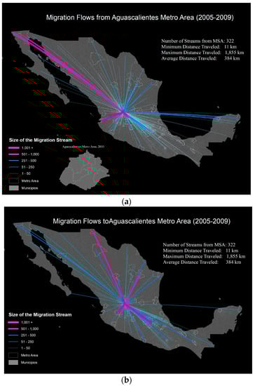
Figure 1.
Spatial distribution of migration flows (a) from, and (b) to the Aguascalientes metropolitan area, 2005–2009. Notes: map generated using ArcGIS.
As this case illustrates and is fairly common in mobility processes, the vast majority of Mexican municipalities are only connected to a small fraction of all possible destinations. Indeed, while intermunicipal flows range from 0 to just under 54,000, only 1.5% of all possible bilateral flows yielded nonzero values.
To further demonstrate overall mobility, Figure 2 shows a circular plot of movement between metropolitan, urban non-metro (i.e., micropolitan), and rural municipalities. While we have grouped municipalities here by degree of urbanization, this plot could be produced for any set of municipalities, regions, and so forth. The key element is the migration stream itself between locations of origin and destination.
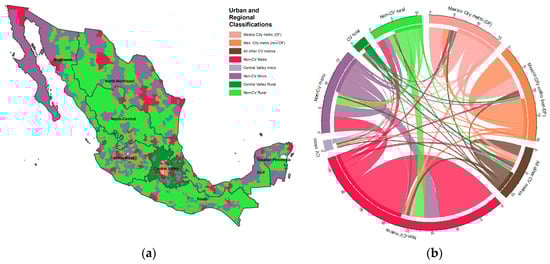
Figure 2.
(a) Municipal classification map of Mexico and (b) flows of migrants between them, 2005–2009. Note: Base of the plot pertains to both region of origin (flows from part of base with no white gap) and destination (flows ending in part of the base with white gap). Size of flow indicated in 10,000s. Map generated using ArcGIS; Circoplot generated using the circlize package in R.
4.1. Data Limitations
While useful in many ways—discussed in the next section– these data have several limitations worth keeping in mind. First, these data do not necessarily measure all intermunicipal movement taking place during the retrospective window, as they miss circular or multistage flows occurring within it. By circular movement, we refer to moves from municipality i to municipality j after the start of the window, but where people move back to municipality i before the end of the window, thus appearing as if they had not moved during the observation period as their municipality of residence five years prior is the same as their place of residence at the time of the Census. By multistage flows, we mean those in which people change municipalities two or more times during the window (e.g., from municipality i, to k, to j), which these data would only register as a single move between i and j.
In addition to these clearer limitations, there is also the matter of how these data should be interpreted, even when assuming that they are relatively complete counts of intermunicipal flows. It is common that intermunicipal movement is thought of as one depicting internal “migration” as opposed to more limited residential mobility processes [13,14]. Yet, these measures include a mix of both processes given that some residential moves happen to cross municipal boundaries—in the Mexican context, this is particularly likely in intermunicipal moves occurring within metropolitan areas [14]. Perhaps more importantly, intermunicipal movement does not include all types of migration (and most certainly of residential mobility) as many such moves occur within municipal boundaries. Unfortunately, in most contexts, there are no data that allow for an empirical assessment of whether unobserved intra-municipal moves are sizable enough to affect estimates of gridded population redistributions. Nevertheless, the reader should be warned that almost any existing “internal migration” data only encompass moves between secondary administrative units like municipalities [5] and that most residential mobility data measures moves occurring within the same locality or place, without recording the prior location of the move. Finally, note that migration measures are the only ones taken retrospectively in Censuses and surveys. As such, the vast majority of demographic, social, and economic characteristics –indeed, measured at the time of interview only—may have changed as a result of the migration and thus are endogenous to mobility. This complicates the use of covariates in analyses of mobility, which is something that ameliorate by aggregating data at the municipal level and/or using lagged aggregate characteristics from a different source.
4.2. Data Format and Applications to Gridded Population Products
As is probably evident by now, these data are fundamentally point data that require further processing to be allocated into a grid or raster either as the main output (e.g., how many people left/moved into a particular grid location) or as inputs to populate/interpolate other gridded products (e.g., population size and age-sex structures). Indeed, as discussed before, the coarser spatial resolution of these and most migration data around the world does not allow for a precise spatial allocation of where people are moving to and from beyond municipalities. Without these more exact locations, GIS scientists are left with the massive challenge of transposing data on administrative/Census units into a grid when estimating present and projected spatial population distributions. Given the litany of problems related to identifying migrant flows over space (noted above), it is unsurprising that this problem is pronounced in the case of migration, and gridded projections of future populations may suffer from a lack of relevant information regarding internal migration patterns.
Despite these challenges, retrospective migration data of the type presented here offer the potential to be used in other studies of migration, to understand the drivers of migration [14]. One such study in the United States uses county-to-county migration to estimate a potential migration response to sea-level rise in the United States [15]. Furthermore, migration -especially internal mobility- has been absent from most of the estimates and forecasts of population futures in the context of climate change. A recent study by the World Bank studying the implications of climate change for populations as a risk of its consequences [16] aims to address this issue. However, because of the lack of data on intermunicipal populations around much of the world, the study used an indirect method of residual population change in order to estimate migration flows. Direct flow data, such as those we have produced here, allow for a direct (and thus overall higher-quality) estimation not just of those flows, but of the characteristics of the migration flows described before.
In addition to these applications, migration data have also proven useful in improving gridded population products, very much including dynamic, gravity-based spatial models of high-resolution, future population scenarios [17]. To demonstrate, consider the recently released spatially explicit population projections of the shared socioeconomic pathways (SSPs), a set of future scenarios used by the global climate-change community [18]. These projections are constructed using a gravity-based downscaling model that assesses the relative attractiveness of grid cells of a 1/8th degree resolution as a function of observed historic change and different demographic, socioeconomic, and geographic indicators. For purposes of consistency across countries, data regarding internal migration patterns were not considered because, for the majority of countries, there are no historical data against which to calibrate the model (see also [5]]. Indeed, note that Mexico only begun collecting intermunicipal (as opposed to interstate) mobility data in the 2000 Census, continuing with this collection in 2010, but not in its large “Inter-Census” surveys in 2005 and 2015 (though reportedly the question will be included again in the 2020 Census).
In contrast, an alternative spatial projection for Mexico, based on a state-level aggregate population projection produced by the Mexican National Population Council (MNPC), did consider state-level internal migration projections in applying a similar gravity-based model [19]. While this projection did not consider movement between municipalities –which would have yielded a much higher resolution in our estimates– there are noticeable differences in outcomes for the year 2050 under two similar scenarios (MNCP and SSP2, scaled such that total population is the same in both). Figure 3 illustrates the difference in projected population density (2050) under the MNCP and SSP2 scenarios (expressed as the expected density under the MNCP scenario minus the expected density under SSP2). The MNCP scenario projects significantly higher populations along the Pacific Coast, Tabasco and Chiapas states, and the Yucatan in the Southeast, and in cities such as Monterey and Tijuana. Conversely, the same scenario projects a smaller population in the state of Jalisco and its capital city Guadalajara. Of particular interest are the contrasting projections in the greater Mexico City area. The SSP2 model projects very high populations in the Distrito Federal, while the MNCP model moves the bulk of the projected population growth in the area into suburban space, particularly in the state of Mexico. Both aggregate-level projections were produced using the same cohort-component method, and included only very minor differences in fertility/mortality assumptions (resulting in a 2050 total population of 151 million under SSP2 and 148 million under the MNCP scenario). Because the SSPs include no consideration of internal migration, it can be concluded that the primary source of variation between the two 2050 scenarios is, in fact, internal migration. Such substantial differences have important planning and policy implications. Relatedly, it is important to note that the exclusion of intrastate migration from these calculations may also yield more conservative change in the grids of particular states where mobility within them is large and dynamic, e.g., as they contain several metropolitan areas within them. This is perhaps especially the case of the State of Mexico in the Central-Southern part of the country.
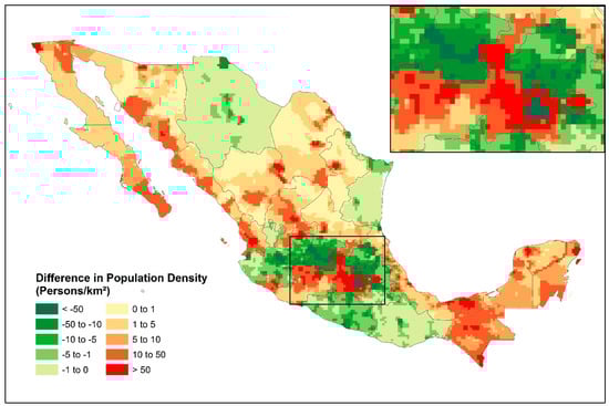
Figure 3.
Difference in projected population density between the Mexican National Population Council and Shared Socioeconomic Pathway 2 scenarios for Mexico (2050).
Notes: Map Produced Using ArcGIS
While historic validation of the gravity-based model is not available for Mexico, its evaluation against US data (1950–2000) indicated a substantial reduction in average error at the grid-cell level [17], highlighting the importance of internal, bilateral flow data in fine-tuning gravity-type approaches to producing gridded population projections. In addition, while it is important to consider how future migration patterns are likely to resemble or deviate from those of the past at different spatial scales (i.e., how should historic data integrate into models of future outcomes), the municipal flows presented in this work are likely to significantly improve projections for Mexico beyond even the MNCP scenario illustrated in Figure 3 given the high degree of spatial detail in the data.
Supplementary Materials
The following are available online at https://zenodo.org/record/2673275#.XRbLUb6YOpp.
Author Contributions
Conceptualization, D.B., F.R., and B.J.; methodology, B.J., D.H.S., and F.R.; software/coding, D.H.S. and F.R.; validation, B.J. and D.H.S.; formal analysis, B.J., D.H.S., and F.R.; investigation, F.R..; resources, D.B. and F.R.; data curation, D.H.S. and F.R.; writing—original draft preparation, D.B. and F.R.; writing—review and editing, B.J., D.B., F.R., and D.H.S.; visualization, D.B. and B.J.; supervision, F.R.; project administration, D.B.; funding acquisition, D.B.
Funding
This research was funded by NSF grant no. 1416860 (PI: Balk) and by an Andrew Carnegie Fellowship from the Carnegie Corporation of New York to Deborah Balk (G-F-16-53680). We also acknowledge support to Simon from the National Science Foundation Graduate Research Fellowship Program (Grant 1416960). Further, we acknowledge research, administrative, and computing support to Riosmena and Simon by the University of Colorado Population Center (Project 2P2CHD066613-06), funded by the Eunice Kennedy Shriver National Institute of Child Health and Human Development. This work also benefited from dialogue at the CUPC Conference on Climate Change, Migration and Health (NICHD project 5R13HD078101).
Acknowledgments
We thank Anastasia Clark and Elizabeth Major for research assistance.
Conflicts of Interest
The authors declare no conflict of interest. The funders had no role in the design of the study; in the collection, analyses, or interpretation of data; in the writing of the manuscript; or in the decision to publish the results.
Appendix A. Stata Code Used to Create Total and Sex-Specific Intermunicipal and Interstate Origin-Destination Matrices from IPUMS International Publicly-Available Data
* ==============================================================================
* File: MigrationStreamCreation.do
* Created by: Daniel H. Simon & Fernando Riosmena (University of Colorado)
* Date: November 30, 2018
* Last Updated: January 20, 2019
* Description: DO FILE FOR CREATION OF INTERNAL MIGRATION STREAMS
* ==============================================================================
* Code for DATA submission, “ Estimating internal migration in contemporary Mexico: //
// The missing link in understanding spatial distributions of population”
* Data Used: Mexican census data (2000 & 2010) obtained through IPUMS-International extract system, which is public use //
// and available at https://international.ipums.org/international/
* ==============================================================================
* LOADING AND CLEANING IPUMS DATA
* ==============================================================================
clear //clear existing data
clear matrix //clear stored data in STATA memory
set more off, permanent
/* Replace with file path for IPUMS extract, or place IPUMS extract in same directory as do file */
cd “.”
/* Replace with Name of dataset with Raw census data */
use “IPUMSMX2000-2010.dta”
/* As per the IPUMS International user agreement, original raw needs to be directly downloaded by any interested user from IPUMS International */
/* Here, we present the code needed to aggregate flows (which can also be adapted to many other countries with minor adjustments (e.g., geocodes) */
/* while indeed sharing the final output aggregated data */
* 5-YEAR MIGRATION QUESTION N/A FOR CHILDREN UNDER 5
drop if age<5
* STATE AND MUNICIPALITY OF ORIGIN/DESTINATION
gen STATE_dest=. // Generate state of destination variables for each census year
replace STATE_dest=GEOLEV1 //Harmonized, first administrative division boundary
gen STATE_orig=. // Creating state of origin from variable that identifies “State or country of residence in 1995 for 2000 Census & 2005 for 2010 Census”
replace STATE_orig=mx2000a_resent if year==2000 & mx2000a_resent>=1 & mx2000a_resent<=32
replace STATE_orig=0 if year==2000 & mx2000a_resent>32 & mx2000a_resent<999
replace STATE_orig=mx2010a_migstat5 if year==2010 & mx2010a_migstat5>=1 & mx2010a_migstat5<=32 // Same procedure for 2005
replace STATE_orig=0 if year==2010 & mx2010a_migstat5==97
/* Note that this variable is NOT harmonized across IPUMS, so need to download one specific to each country-period of interest */
gen MUNID_dest=.
replace MUNID_dest=GEO_LEV2 //Harmonized, second administrative division boundary
gen MUNID_orig=.
replace MUNID_orig=STATE_orig*1000+mx2000a_resmun if year==2000 & STATE_orig>0 & STATE_orig<33
replace MUNID_orig=mx2010a_migmuni5 if year==2010 & mx2010a_migmuni5>=1001 & mx2010a_migmuni5<=32999
replace MUNID_orig=0 if STATE_orig==0
/* Note that this variable is NOT harmonized across IPUMS, so need to download one specific to each country-period of interest */
// 999 CODE IDENTIFIES INDIVIDUALS WITH UNKNOWN MUNICIPALITY OF ORIGIN
replace MUNID_orig=. if MUNID_orig==99998
replace MUNID_orig=. if MUNID_orig==1999
replace MUNID_orig=. if MUNID_orig==2999
replace MUNID_orig=. if MUNID_orig==3999
replace MUNID_orig=. if MUNID_orig==4999
replace MUNID_orig=. if MUNID_orig==5999
replace MUNID_orig=. if MUNID_orig==6999
replace MUNID_orig=. if MUNID_orig==7999
replace MUNID_orig=. if MUNID_orig==8999
replace MUNID_orig=. if MUNID_orig==9999
replace MUNID_orig=. if MUNID_orig==10999
replace MUNID_orig=. if MUNID_orig==11999
replace MUNID_orig=. if MUNID_orig==12999
replace MUNID_orig=. if MUNID_orig==13999
replace MUNID_orig=. if MUNID_orig==14999
replace MUNID_orig=. if MUNID_orig==15999
replace MUNID_orig=. if MUNID_orig==16999
replace MUNID_orig=. if MUNID_orig==17999
replace MUNID_orig=. if MUNID_orig==18999
replace MUNID_orig=. if MUNID_orig==19999
replace MUNID_orig=. if MUNID_orig==20999
replace MUNID_orig=. if MUNID_orig==21999
replace MUNID_orig=. if MUNID_orig==22999
replace MUNID_orig=. if MUNID_orig==23999
replace MUNID_orig=. if MUNID_orig==24999
replace MUNID_orig=. if MUNID_orig==25999
replace MUNID_orig=. if MUNID_orig==26999
replace MUNID_orig=. if MUNID_orig==27999
replace MUNID_orig=. if MUNID_orig==28999
replace MUNID_orig=. if MUNID_orig==29999
replace MUNID_orig=. if MUNID_orig==30999
replace MUNID_orig=. if MUNID_orig==31999
replace MUNID_orig=. if MUNID_orig==32999
* IDENTIFY MIGRANTS FOR STREAMS OFF HARMONIZED VARIABLE
// 10: Same major admin. unit; 11: Same major, same minor; 12: Same major, different minor; 20: Diferent major; 30: Abroad; 99: Missing
gen migrant=0
replace migrant=1 if migrate5==10
replace migrant=1 if migrate5==12
replace migrant=1 if migrate5==20
replace migrant=1 if migrate5==30
replace migrant=. if migrate5==99
// Create identifier for inter-state migrants only
gen interstatemig = 0
replace interstatemig=1 if migrate5==20
replace interstatemig=. if migrate5==99
// Create migrant sex identifiers for flows by sex
// User can modify to stratify flows by e.g., age, schooling levels or the like
// Beware, however, that these measurements are *after* migration,
// so either need to assume no changes in e.g., schooling,
// or adjust for the time change (in e.g., age)
gen migrantmale=0
replace migrantmale=1 if sex==1 & migrant==1
replace migrantmale=. if migrant==. | sex==.
gen migrantfem=0
replace migrantfem=1 if sex==2 & migrant==1
replace migrantfem=. if migrant==. | sex==.
keep MUNID_* STATE_* year migrant* interstatemig perwt
// Saving dataset with basic info to recall for different calculations
save “IPUMS_DatatoCollapse.dta”,replace
* ==============================================================================
* CREATE MUNICIPAL MIGRATION STREAMS FROM INDIVIDUAL IPUMS DATA
* ==============================================================================
* TO AGGREGATE DATA, COLLAPSE MIGRANTS BY MUNICIPALITIES TO GET MIGRANT COUNTS
// All migrants for total flows
clear all
use “IPUMS_DatatoCollapse.dta”
collapse (count) migrants=migrant ///
[pweight=perwt] if migrant==1, by (STATE_dest MUNID_dest STATE_orig MUNID_orig year)
// Technically, don’t need to include both STATE and MUNID identifiers if GEOLEVEL2 is unique for each country
// However, beware if this is not the case
// Also, if you are using more than 1 country, will need to add country variable
// to every by() procedure from here on out.
// Don’t want to count people moving from municipalities that were created in 2005-2010 to the municipalities they were created from
drop if MUNID_orig==MUNID_dest
replace STATE_orig=0 if MUNID_orig==0
sort MUNID_orig MUNID_dest year
save “IntermunicipalFlows.dta”, replace
//Aggregating flows by sex
// Male Migrant Flows
clear all
use “IPUMS_DatatoCollapse.dta”
collapse (count) malemigrants=migrantmale ///
[pweight=perwt] if migrantmale==1, by (STATE_dest MUNID_dest STATE_orig MUNID_orig year)
drop if MUNID_orig==MUNID_dest
replace STATE_orig=0 if MUNID_orig==0
sort MUNID_orig MUNID_dest year
save “IntermunicipalMaleFlows.dta”, replace
// Female Migrant Flows
clear all
use “IPUMS_DatatoCollapse.dta”
collapse (count) femalemigrants=migrantfem ///
[pweight=perwt] if migrantfem==1, by (STATE_dest MUNID_dest STATE_orig MUNID_orig year)
// This gets rid of people moving from municipalities that were created in 2005-2010 to the municipalities they were created from...
drop if MUNID_orig==MUNID_dest
replace STATE_orig=0 if MUNID_orig==0
sort MUNID_orig MUNID_dest year
save “IntermunicipalFemaleFlows.dta”, replace
* ==============================================================================
* MERGING MUNICIPAL FLOW DATA
* ==============================================================================
// Note we also create a “frame” with all possible combinations of
// intermunicipal flows to merge the data to
// This is helpful in order to assign zeroes to any origin-destination
// dyad without any data.
// Otherwise, output dataset would not yield as many origin-destination
// dyads as theoretically possible.
clear
use “IntermunicipalFlows.dta”
sort MUNID_orig MUNID_dest year
merge m:m MUNID_orig MUNID_dest year using “IntermunicipalMaleFlows.dta”, keepusing(malemigrants)
rename _merge _mergeMALEmig
replace malemigrants=0 if malemigrants==. & migrants>=0
merge m:m MUNID_orig MUNID_dest year using “IntermunicipalFemaleFlows.dta”, keepusing(femalemigrants)
rename _merge _mergeFEMALEmig
replace femalemigrants=0 if femalemigrants==. & migrants>=0
//Only keeping internal migration in this file (0 is code for international origins/destinations)
drop if MUNID_orig==0 | MUNID_dest==0
merge m:m MUNID_orig MUNID_dest year using MuniOriginDestFrame.dta, keepusing(MUNID_orig STATE_orig MUNID_dest STATE_dest)
// Dataset has entries for unknown origin for many destinations, including those with known state of prior residence but unknown muni...
// Assigning all dyads in which no one in Census
/// reported moving to and from as 0
foreach var of varlist *migrants* {
replace ‘var’=0 if _merge==2
}
rename _merge _mergeFRAME
keep year STATE_orig MUNID_orig STATE_dest MUNID_dest migrants malemig* female*
save “CompleteIntermunicipalFlows.dta”, replace
outsheet using "“CompleteIntermunicipalFlows.csv”, comma replace
* ==============================================================================
* CREATE INTERSTATE MIGRATION STREAMS FROM INDIVIDUAL IPUMS DATA (separate file)
* ==============================================================================
clear all
use “CompleteIntermunicipalFlows.dta”
drop if MUNID_orig==0 | MUNID_dest==0
collapse (sum) interstatemigrants=migrants, by (STATE_dest STATE_orig year)
drop if STATE_orig==STATE_dest // could keep if interested in no. of intrastate moves
save “InterstateMigrationFlows.dta”,replace
// Interstate flows by sex
// Male flows
clear
use “CompleteIntermunicipalFlows.dta”
drop if MUNID_orig==0 | MUNID_dest==0
collapse (sum) interstatemalemig=malemigrants, by (STATE_dest STATE_orig year)
drop if STATE_orig==STATE_dest // could keep if interested in no. of intrastate moves
save “InterstateMaleFlows.dta”,replace
// Female flows
clear
use “CompleteIntermunicipalFlows.dta”
drop if MUNID_orig==0 | MUNID_dest==0
collapse (sum) interstatefemalemig=femalemigrants, by (STATE_dest STATE_orig year)
drop if STATE_orig==STATE_dest // could keep if interested in no. of intrastate moves
save “InterstateFemaleFlows.dta”,replace
* ==============================================================================
* MERGING INTERSTATE FLOW DATA (no need for data frame as state-to-state flows are complete in data)
* ==============================================================================
clear
use “InterstateMigrationFlows.dta”
merge m:m STATE_dest STATE_orig year using “InterstateMaleFlows.dta”, keepusing(interstatemalemig)
rename _merge _mergeMALEmig
replace interstatemalemig=0 if interstatemalemig==. & interstatemigrants>=0
merge m:m STATE_dest STATE_orig year using “InterstateFemaleFlows.dta”, keepusing(interstatefemalemig)
rename _merge _mergeFEMALEmig
replace interstatefemalemig=0 if interstatefemalemig==. & interstatemigrants>=0
//Keeping only domestic destinations
drop if STATE_dest==0 | STATE_orig==0
sort STATE_dest STATE_orig year
save “CompleteInterstateFlows.dta”,replace
outsheet using “CompleteInterstateFlows.csv”, comma replace
References
- Jones, B.; O’Neill, B.C.; McDaniel, L.; McGinnis, S.; Mearns, L.O.; Tebaldi, C. Future population exposure to US heat extremes. Nat. Clim. Chang. 2015, 5, 652. [Google Scholar] [CrossRef]
- Tatem, A.J. WorldPop, open data for spatial demography. Sci. Data 2017, 4, 170004. [Google Scholar] [CrossRef] [PubMed]
- Ruggles, S.; Alexander, J.T.; Genadek, K.; Goeken, R.; Schroeder, M.B.; Sobek, M. Integrated Public Use Microdata Series: Version 5.0 [Machine-Readable Database]; University of Minnesota: Minneapolis, MN, USA, 2010. [Google Scholar]
- Ruggles, S.; Manson, S.M.; Kugler, T.A.; Haynes, D.A., II; Van Riper, D.C.; Bakhtsiyarava, M. IPUMS Terra: Integrated Data on Population and Environment: Version 2 [Dataset]; IPUMS: Minneapolis, MN, USA, 2018. [Google Scholar] [CrossRef]
- Bell, M.; Charles-Edwards, E.; Kupiszewska, D.; Kupiszewski, M.; Stillwell, J.; Zhu, Y. Internal migration data around the world: Assessing contemporary practice. Popul. Space Place 2015, 21, 1–17. [Google Scholar] [CrossRef]
- INEGI. Síntesis metodológica del XII Censo General de Población y Vivienda. 2000. Available online: http://internet.contenidos.inegi.org.mx/contenidos/Productos/prod_serv/contenidos/espanol/bvinegi/productos/metodologias/est/702825000014.pdf (accessed on 8 April 2018).
- INEGI. Censo de Población y Vivienda 2010: Diseño de la Muestra Censal. 2010. Available online: http://internet.contenidos.inegi.org.mx/contenidos/Productos/prod_serv/contenidos/espanol/bvinegi/productos/metodologias/est/dis_muestra_cpv2010.pdf (accessed on 8 April 2018).
- Sorichetta, A.; Bird, T.J.; Ruktanonchai, N.W.; Zu Erbach-Schoenberg, E.; Pezzulo, C.; Tejedor, N.; Waldock, I.; Sadler, J.D.; Garcia, A.J.; Seda, L.; et al. Mapping internal connectivity through human migration in malaria endemic countries. Sci. Data 2016, 3, 160066. [Google Scholar] [CrossRef] [PubMed]
- Pérez Campuzano, E.; Santos Cerquera, C. Tendencias recientes de la migración interna en México. Pap. Población 2013, 19, 53–88. [Google Scholar]
- The Image Project: Comparing Internal Migration Around the Globe: Project Framework. Available online: https://imageproject.com.au/framework/ (accessed on 29 March 2019).
- Censo General de Población y Vivienda 2000: Conjunto de datos: Población de 5 y más años. Available online: https://www.inegi.org.mx/sistemas/olap/proyectos/bd/censos/cpv2000/p5.asp?s=est&c=10262&proy=cpv00_p5 (accessed on 20 January 2019).
- Censo General de Población y Vivienda 2010. Available online: https://www.inegi.org.mx/sistemas/olap/proyectos/bd/censos/cpv2010/p3mas.asp?s=est&c=27781&proy=cpv10_p3mas (accessed on 20 January 2019).
- Sobrino, J. Patrones de dispersión intrametropolitana en México. Estud. Demog. Urbanos 2007, 22, 583–617. [Google Scholar] [CrossRef]
- Riosmena, F.; Balk, D. Internal Migration and other Mobility in Contemporary Mexico: Understanding Their Dynamics and Drivers Using Alternative Flow Typologies. 2019, Unpublished manuscript. 2019; Unpublished manuscript. [Google Scholar]
- Hauer, M. Migration induced by sea-level rise could reshape the US population landscape. Nat. Clim. Chang. 2017, 7, 321–325. [Google Scholar] [CrossRef]
- Rigaud, K.K.; de Sherbinin, A.; Jones, B.; Bergmann, J.; Clement, V.; Ober, K.; Schewe, J.; Adamo, S.; McCusker, B.; Heuser, S.; et al. Groundswell: Preparing for Internal Climate Migration; The World Bank: Washington, DC, USA, 2018. [Google Scholar]
- Jones, B.; O’Neill, B.C. Historically grounded spatial population projections for the continental United States. Environ. Res. Lett. 2013, 8, 044021. [Google Scholar] [CrossRef]
- Jones, B.; O’Neill, B.C. Spatially explicit global population scenarios consistent with the Shared Socioeconomic Pathways. Environ. Res. Lett. 2016, 11, 084003. [Google Scholar] [CrossRef]
- Proyecciones de la Población de México y de las Entidades Federativas, 2016–2050. Available online: https://datos.gob.mx/busca/dataset/proyecciones-de-la-poblacion-de-mexico-y-de-las-entidades-federativas-2016-2050 (accessed on 20 January 2019).
© 2019 by the authors. Licensee MDPI, Basel, Switzerland. This article is an open access article distributed under the terms and conditions of the Creative Commons Attribution (CC BY) license (http://creativecommons.org/licenses/by/4.0/).