UAV-Based 3D Point Clouds of Freshwater Fish Habitats, Xingu River Basin, Brazil

 ,
, 
 and
and
Abstract
1. Summary
2. Data Description
3. Methods
4. Limitations
5. Conclusions
Author Contributions
Funding
Acknowledgments
Conflicts of Interest
References
- Kalacska, M.; Lucanus, O.; Sousa, L.M.; Vieira, T.; Arroyo-Mora, J.P. Freshwater fish habitat complexity maping using above and underwater structure-from-motion photogrammetry. Remote Sens. 2018, 10, 1912. [Google Scholar] [CrossRef]
- Du Preez, C. A new arc-chord ratio (ACR) rugosity index for quantifying three-dimensional landscape structural complexity. Landsc. Ecol. 2015, 30, 181–192. [Google Scholar] [CrossRef]
- Walbridge, S.; Slocum, N.; Pobuda, M.; Wright, D.J. Unified Geomorphological Analysis Workflows with Benthic Terrain Modeler. Geosciences 2018, 8, 94. [Google Scholar] [CrossRef]
- Reichert, J.; Backes, A.R.; Schubert, P.; Wilke, T. The power of 3D fractal dimensions for comparative shape and structural complexity analyses of irregularly shaped organisms. Methods Ecol. Evol. 2017, 8, 1650–1658. [Google Scholar] [CrossRef]
- Leon, J.X.; Roelfsema, C.M.; Saunders, M.I.; Phinn, S.R. Measuring coral reef terrain roughness using ‘Structure-from-Motion’ close-range photogrammetry. Geomorphology 2015, 242, 21–28. [Google Scholar] [CrossRef]
- McCormick, M.I. Comparison of field methods for measuring surface-topography and their associations with a tropical reef fish assemblage. Mar. Ecol. Prog. Ser. 1994, 112, 87–96. [Google Scholar] [CrossRef]
- Anderson, K.; Gaston, K.J. Lightweight unmanned aerial vehicles will revolutionize spatial ecology. Front. Ecol. Environ. 2013, 11, 138–146. [Google Scholar] [CrossRef]
- Cunliffe, A.M.; Brazier, R.E.; Anderson, K. Ultra-fine grain landscape-scale quantification of dryland vegetation structure with drone-acquired structure-from-motion photogrammetry. Remote Sens. Environ. 2016, 183, 129–143. [Google Scholar] [CrossRef]
- Linchant, J.; Lisein, J.; Semeki, J.; Lejeune, P.; Vermeulen, C. Are unmanned aircraft systems (UASs) the future of wildlife monitoring? A review of accomplishments and challenges. Mammal Rev. 2015, 45, 239–252. [Google Scholar] [CrossRef]
- Micheletti, N.; Chandler, J.H.; Lane, S.N. Structure from Motion (SfM) Photogrammetry. In Geomorphological Techniques; British Society for Geomorphology: London, UK, 2015; pp. 2–12. [Google Scholar]
- House, J.E.; Brambilla, V.; Bidaut, L.M.; Christie, A.P.; Pizarro, O.; Madin, J.S.; Dornelas, M. Moving to 3D: Relationships between coral planar area, surface area and volume. PeerJ 2018, 6, 19. [Google Scholar] [CrossRef]
- Palma, M.; Casado, M.R.; Pantaleo, U.; Cerrano, C. High Resolution Orthomosaics of African Coral Reefs: A Tool for Wide-Scale Benthic Monitoring. Remote Sens. 2017, 9, 705. [Google Scholar] [CrossRef]
- Young, G.C.; Dey, S.; Rogers, A.D.; Exton, D. Cost and time-effective method for multiscale measures of rugosity, fractal dimension, and vector dispersion from coral reef 3D models. PLoS ONE 2017, 12, e0175341. [Google Scholar] [CrossRef] [PubMed]
- Singh, H.; Roman, C.; Pizarro, O.; Eustice, R.; Can, A. Towards high-resolution imaging from underwater vehicles. Int. J. Robot. Res. 2007, 26, 55–74. [Google Scholar] [CrossRef]
- Ferrari, R.; Bryson, M.; Bridge, T.; Hustache, J.; Williams, S.B.; Byrne, M.; Figueira, W. Quantifying the response of structural complexity and community composition to environmental change in marine communities. Glob. Chang. Boil. 2016, 22, 1965–1975. [Google Scholar] [CrossRef] [PubMed]
- Fonseca, V.P.; Pennino, M.G.; de Nobrega, M.F.; Oliveira, J.E.L.; Mendes, L.D. Identifying fish diversity hot-spots in data-poor situations. Mar. Environ. Res. 2017, 129, 365–373. [Google Scholar] [CrossRef]
- Gonzalez-Rivero, M.; Harborne, A.R.; Herrera-Reveles, A.; Bozec, Y.M.; Rogers, A.; Friedman, A.; Ganase, A.; Hoegh-Guldberg, O. Linking fishes to multiple metrics of coral reef structural complexity using three-dimensional technology. Sci. Rep. 2017, 7, 13965. [Google Scholar] [CrossRef] [PubMed]
- Taniguchi, H.; Tokeshi, M. Effects of habitat complexity on benthic assemblages in a variable environment. Freshw. Boil. 2004, 49, 1164–1178. [Google Scholar] [CrossRef]
- ASPRS. LAS Specification v 1.2; ASPRS: Bethesda, MD, USA, 2008. [Google Scholar]
- Dandois, J.P.; Olano, M.; Ellis, E.C. Optimal Altitude, Overlap, and Weather Conditions for Computer Vision UAV Estimates of Forest Structure. Remote Sens. 2015, 7, 13895–13920. [Google Scholar] [CrossRef]
- Kalacska, M.; Chmura, G.L.; Lucanus, O.; Berube, D.; Arroyo-Mora, J.P. Structure from motion will revolutionize analyses of tidal wetland landscapes. Remote Sens. Environ. 2017, 199, 14–24. [Google Scholar] [CrossRef]
- Lowe, D.G. Distinctive image features from scale-invariant keypoints. Int. J. Comput. Vis. 2004, 60, 91–110. [Google Scholar] [CrossRef]
- Strecha, C.; von Hansen, W.; Van Gool, L.; Fua, P.; Thoennessen, U. On Benchmarking camera calibration and multi-view stereo for high resolution imagery. In Proceedings of the 2008 IEEE Conference on Computer Vision and Pattern Recognition, Anchorage, AK, USA, 23–28 June 2008. [Google Scholar]
- Strecha, C.; Bronstein, A.M.; Bronstein, M.M.; Fua, P. LDAHash: Improved Matching with Smaller Descriptors. IEEE Trans. Pattern Anal. Mach. Intell. 2012, 34, 66–78. [Google Scholar] [CrossRef] [PubMed]
- Vautherin, J.; Rutishauser, S.; Schneider-Zapp, K.; Choi, H.F.; Chovancova, V.; Glass, A.; Strecha, C. Photogrammetric accuracy and modeling of rolling shutter cameras. ISPRS J. Photogramm. Remote Sens. 2016, 3, 139–146. [Google Scholar] [CrossRef]
- Tamminga, A.; Hugenholtz, C.; Eaton, B.; Lapointe, M. Hyperspatial remote sensing of channel reach morphology and hydraulic fish habitat using an unmanned aerial vehicle (UAV): A first assessment in the context of river research and management. River Res. Appl. 2015, 31, 379–391. [Google Scholar] [CrossRef]
- Westaway, R.M.; Lane, S.N.; Hicks, D.M. The development of an automated correction procedure for digital photogrammetry for the study of wide, shallow, gravel-bed rivers. Earth Surf. Process. Landf. 2000, 25, 209–226. [Google Scholar] [CrossRef]
- Woodget, A.S.; Carbonneau, P.E.; Visser, F.; Maddock, I.P. Quantifying submerged fluvial topography using hyperspatial resolution UAS imagery and structure from motion photogrammetry. Earth Surf. Process. Landf. 2015, 40, 47–64. [Google Scholar] [CrossRef]


| File | Location | Size | Interactive version |
|---|---|---|---|
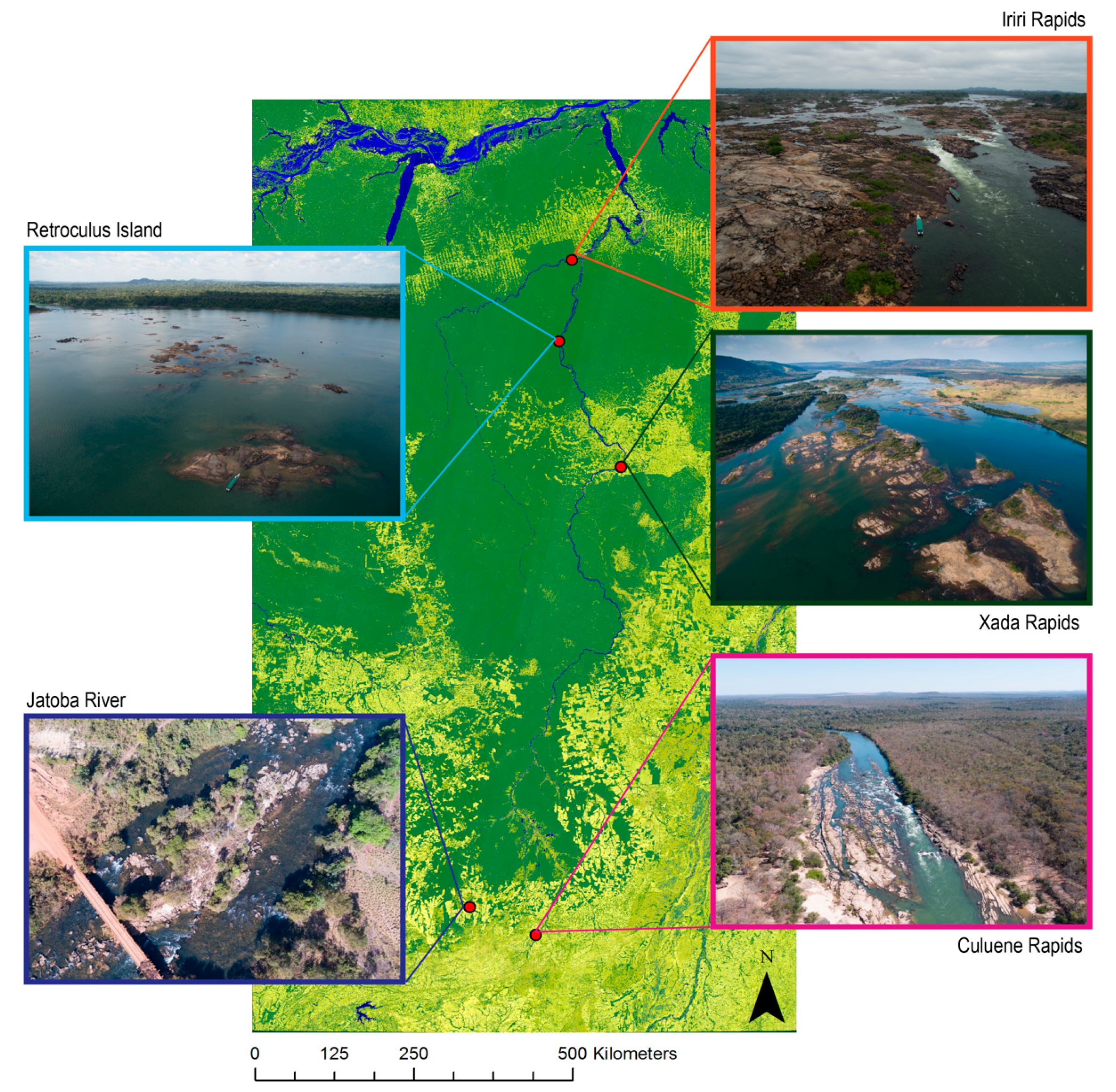
| Jatoba.las | Jatoba river | 1.12 GB | http://bit.ly/riojatoba |
| Culuene_HD.las | Culuene rapids | 801.59 MB | http://bit.ly/culuene |
| Retroculus_island.las | Retroculus island | 714.93 MB | http://bit.ly/retroculus |
| Xada_HD.las | Xada rapids | 459.31 MB | http://bit.ly/xadarapids |
| Iriri_HD.las | Iriri rapids | 2.48 GB | http://bit.ly/iriri3D |
| Location | UAV | Camera | Date | GSD (cm) | No. Photographs | Area (ha) |
|---|---|---|---|---|---|---|
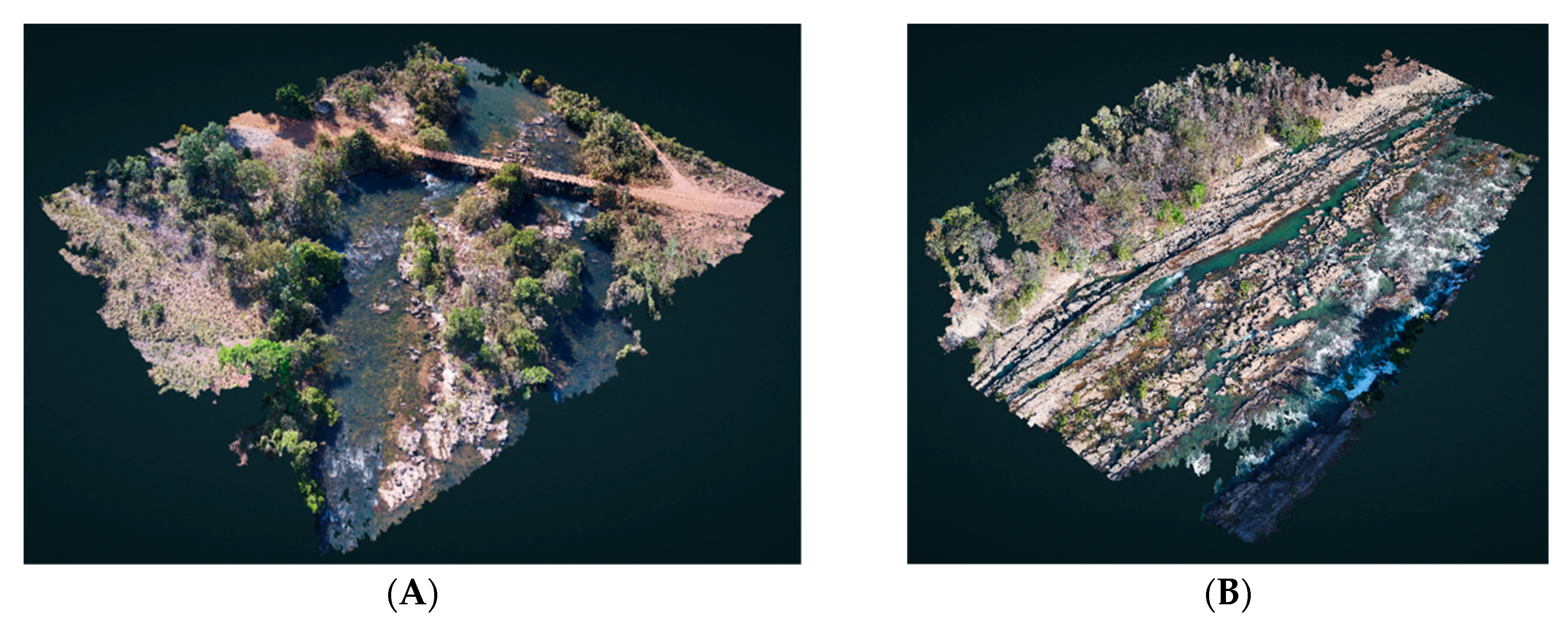
| Jatoba river | Inspire 2 | X5S | 2 August 2017 | 1.20 | 375 | 2.80 |
| Culuene rapids | Inspire 2 | X5S | 1 August 2017 | 1.75 | 283 | 4.54 |
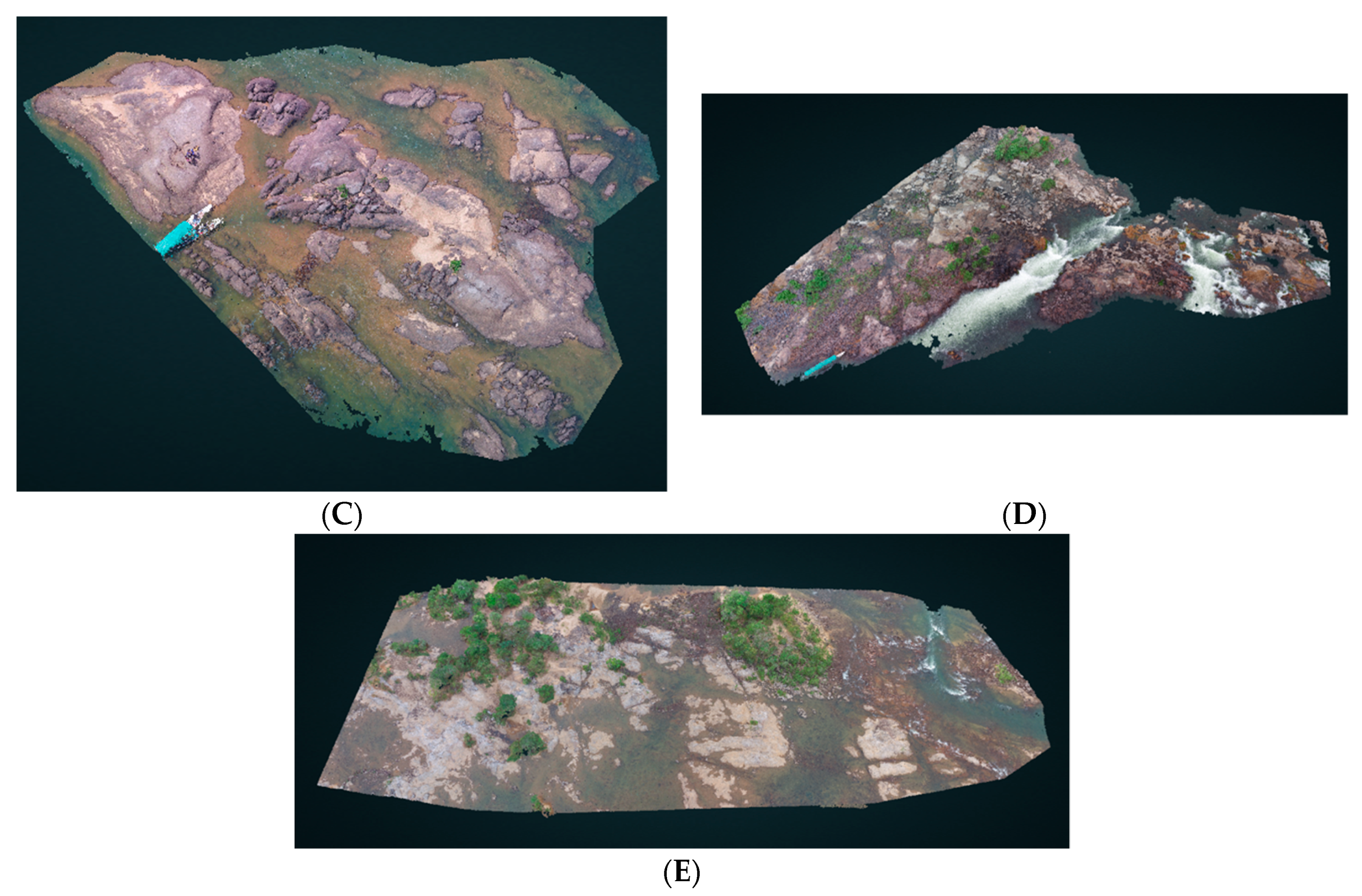
| Retroculus island | Inspire 1 | X3 | 8 August 2016 | 1.43 | 208 | 0.52 |
| Xada rapids | Inspire 1 | X3 | 11 August 2016 | 2.38 | 420 | 4.62 |
| Iriri rapids | Inspire 1 | X3 | 6 August 2016 | 1.46 | 425 | 2.77 |
| Location | Camera Speed (m/s) | Displacement During Readout (m) | Rolling Shutter Readout Time (ms) |
|---|---|---|---|
| Jatoba river | 2.1 | 0.13 | 60.63 |
| Culuene rapids | 3.4 | 0.27 | 80.06 |
| Retroculus island | 2.0 | 0.16 | 80.90 |
| Xada rapids | 2.4 | 0.15 | 63.58 |
| Iriri rapids | 2.0 | 0.14 | 72.29 |
| Location | Median Matches per Image | Avg Point Cloud Density (/m3) | Median Keypoints per Image | Camera Optimization (%) | Total Processing Time | Total Number of Points (Dense Point Cloud) |
|---|---|---|---|---|---|---|
| Jatoba river | 17,958.3 | 1044.0 | 72,446 | 0.33 | 8 h:49 min:58 s | 35,432,692 |
| Culuene rapids | 23,869.7 | 620.6 | 70,893 | 1.96 | 6 h:16 min:04s | 24,695,393 |
| Retroculus Isl. | 23,059.0 | 1782.1 | 5342 | 1.36 | 21 min:44 s | 22,033,200 |
| Xada rapids | 18,118.6 | 469.3 | 41,835 | 3.42 | 1 h:57 min:08 s | 14,129,408 |
| Iriri rapids * | 15,684.2 | 5863.4 | 42,048 | 0.12 | 25 h:58 min:06 s | 78,332,198 |
| Location | X: μ ± σ | Y: μ ± σ | Z: μ ± σ |
|---|---|---|---|
| Jatoba river | 0.00 ± 0.99 | 0.00 ± 0.89 | 0.01 ± 0.32 |
| Culuene rapids | 0.00 ± 1.34 | 0.00 ± 1.86 | 0.00 ± 2.37 |
| Retroculus Island | 0.01 ± 0.52 | 0.00 ± 0.50 | 0.00 ± 1.01 |
| Xada rapids | 0.00 ± 0.89 | 0.00 ± 0.87 | 0.00 ± 0.69 |
| Iriri rapids | 0.00 ± 0.60 | 0.00 ± 0.60 | 0.00 ± 1.00 |
| Location | X (m) | Y (m) | Z (m) | Omega (°) | Phi (°) | Kappa (°) |
|---|---|---|---|---|---|---|
| Jatoba river | 0.008 ± 0.003 | 0.007 ± 0.003 | 0.004 ± 0.001 | 0.012 ± 0.004 | 0.010 ± 0.004 | 0.003 ± 0.001 |
| Culuene rapids | 0.012 ± 0.009 | 0.012 ± 0.008 | 0.005 ± 0.003 | 0.012 ± 0.008 | 0.010 ± 0.007 | 0.004 ± 0.002 |
| Retroculus Isl. | 0.003 ± 0.001 | 0.003 ± 0.001 | 0.002 ± 0.001 | 0.006 ± 0.002 | 0.006 ± 0.002 | 0.003 ± 0.001 |
| Xada rapids | 0.004 ± 0.002 | 0.004 ± 0.002 | 0.003 ± 0.001 | 0.005 ± 0.002 | 0.005 ± 0.002 | 0.002 ± 0.001 |
| Iriri rapids | 0.054 ± 0.032 | 0.053 ± 0.026 | 0.022 ± 0.010 | 0.102 ± 0.048 | 0.097 ± 0.059 | 0.025 ± 0.008 |
| Location | No. 2D Keypoint Observations for Bundle Block Adjustment | No. 3D pts for Bundle Block Adjustment | Mean Reprojection Error (pixels) |
|---|---|---|---|
| Jatoba river | 7,021,320 | 2,165,893 | 0.205 |
| Culuene rapids | 6,436,758 | 1,293,024 | 0.198 |
| Retroculus Island | 1,353,973 | 270,069 | 0.212 |
| Xada rapids | 7,668,646 | 1,442,876 | 0.259 |
| Iriri rapids | 7,720,544 | 1,848,706 | 0.199 |
| Location | Focal Length | Principal Point x | Principal Point y | R1 | R2 | R3 | T1 | T2 |
|---|---|---|---|---|---|---|---|---|
| Jatoba river | I = 15.000 O = 15.065 σ = 0.006 | I = 8.75 O = 8.824 σ = 0.000 | I = 6.556 O = 6.635 σ = 0.002 | I = 0.000 O = −0.005 σ = 0.000 | I = 0.000 O = −0.004 σ = 0.000 | I = −0.000 O = 0.010 σ = 0.001 | I = 0.000 O = 0.001 σ = 0.000 | I = 0.000 O = 0.002 σ = 0.000 |
| Culuene rapids | I = 15.000 O = 14.751 σ = 0.004 | I = 8.75 O = 8.854 σ = 0.000 | I = 6.556 O = 6.764 σ = 0.002 | I = 0.000 O = −0.006 σ = 0.000 | I = 0.000 O = −0.004 σ = 0.000 | I = −0.000 O = 0.010 σ = 0.000 | I = 0.000 O = 0.001 σ = 0.000 | I = 0.000 O = 0.002 σ = 0.000 |
| Retroculus Island | I = 3.61 O = 3.659 σ = 0.002 | I = 3.159 O = 3.157 σ = 0.000 | I = 2.369 O = 2.356 σ = 0.000 | I = −0.13 O = −0.131 σ = 0.000 | I = 0.106 O = 0.108 σ = 0.000 | I = −0.016 O = −0.014 σ = 0.000 | I = 0.000 O = −0.001 σ = 0.000 | I = 0.000 O = 0.000 σ = 0.000 |
| Xada rapids | I = 3.61 O = 3.486 σ = 0.001 | I = 3.159 O = 3.156 σ = 0.000 | I = 2.369 O = 2.352 σ = 0.000 | I = −0.13 O = −0.119 σ = 0.000 | I = 0.106 O = 0.087 σ = 0.000 | I = −0.016 O = −0.009 σ = 0.000 | I = 0.000 O = −0.001 σ = 0.000 | I = 0.000 O = 0.000 σ = 0.000 |
| Iriri rapids | I = 3.551 O = 3.547 σ = 0.000 | I = 3.085 O = 3.084 σ = 0.000 | I = 2.314 O = 2.300 σ = 0.000 | I = −0.13 O = −0.119 σ = 0.000 | I = 0.106 O = 0.104 σ = 0.001 | I = −0.016 O = −0.013 σ = 0.000 | I = 0.000 O = −0.001 σ = 0.000 | I = 0.000 O = 0.000 σ = 0.000 |
© 2019 by the authors. Licensee MDPI, Basel, Switzerland. This article is an open access article distributed under the terms and conditions of the Creative Commons Attribution (CC BY) license (http://creativecommons.org/licenses/by/4.0/).
Share and Cite
Kalacska, M.; Lucanus, O.; Sousa, L.; Vieira, T.; Arroyo-Mora, J.P. UAV-Based 3D Point Clouds of Freshwater Fish Habitats, Xingu River Basin, Brazil. Data 2019, 4, 9. https://doi.org/10.3390/data4010009
Kalacska M, Lucanus O, Sousa L, Vieira T, Arroyo-Mora JP. UAV-Based 3D Point Clouds of Freshwater Fish Habitats, Xingu River Basin, Brazil. Data. 2019; 4(1):9. https://doi.org/10.3390/data4010009
Chicago/Turabian StyleKalacska, Margaret, Oliver Lucanus, Leandro Sousa, Thiago Vieira, and Juan Pablo Arroyo-Mora. 2019. "UAV-Based 3D Point Clouds of Freshwater Fish Habitats, Xingu River Basin, Brazil" Data 4, no. 1: 9. https://doi.org/10.3390/data4010009
APA StyleKalacska, M., Lucanus, O., Sousa, L., Vieira, T., & Arroyo-Mora, J. P. (2019). UAV-Based 3D Point Clouds of Freshwater Fish Habitats, Xingu River Basin, Brazil. Data, 4(1), 9. https://doi.org/10.3390/data4010009