A Cluster Graph Approach to Land Cover Classification Boosting

Abstract

When it comes to land cover classification, the process of deriving the land classes is complex due to possible errors in algorithms, spatio-temporal heterogeneity of the Earth observation data, variation in availability and quality of reference data, or a combination of these. This article proposes a probabilistic graphical model approach, in the form of a cluster graph, to boost geospatial classifications and produce a more accurate and robust classification and uncertainty product. Cluster graphs can be characterized as a means of reasoning about geospatial data such as land cover classifications by considering the effects of spatial distribution, and inter-class dependencies in a computationally efficient manner. To assess the capabilities of our proposed cluster graph boosting approach, we apply it to the field of land cover classification. We make use of existing land cover products (GlobeLand30, CORINE Land Cover) along with data from Volunteered Geographic Information (VGI), namely OpenStreetMap (OSM), to generate a boosted land cover classification and the respective uncertainty estimates. Our approach combines qualitative and quantitative components through the application of our probabilistic graphical model and subjective expert judgments. Evaluating our approach on a test region in Garmisch-Partenkirchen, Germany, our approach was able to boost the overall land cover classification accuracy by 1.4% when compared to an independent reference land cover dataset. Our approach was shown to be robust and was able to produce a diverse, feasible and spatially consistent land cover classification in areas of incomplete and conflicting evidence. On an independent validation scene, we demonstrated that our cluster graph boosting approach was generalizable even when initialized with poor prior assumptions.

1. Introduction

The rapid development of remote sensing techniques and data processing algorithms has led to the availability of large amounts of Earth observation data at regular intervals. However, the usefulness of this data is limited to a small community of experts. Therefore, practical data analysis methods and applications based on remote sensing data have become an active area of research, specifically thematic mapping and land cover classification [1,2,3]. Land cover has been recognized as a key variable in environmental studies for deforestation, climate assessment, food, and water security, and urban growth [4,5].

Due to its high relevance, the demand for accurate and timely production of land cover classification has grown rapidly as governments push towards large-scale, and frequent monitoring of agricultural and urban environments [6]. While a magnitude of approaches exists for creating land cover classifications, the quality, resolution, and reclassification periods for these vary drastically [7,8,9,10]. Additionally, many of these approaches make use of supervised learning where accurately labeled training data is required. This data is often manually annotated and thus suffers from human biases and varying accuracy. Furthermore, as the quality, and quantity of this data directly affects the accuracy of the final classifier the usability of these approaches is often limited to regions which depict similar features to the training dataset.

Overall, land cover classification is an inherently nuanced problem and has a large scope for error. These errors can largely be attributed to automated classification algorithm errors, temporal and spatial heterogeneity of Earth observation data, variation in the availability and quality of reference data, the need for human intervention in labeling. Therefore, trade-offs are required to produce ‘good enough’ land cover classifications. Thus, it becomes clear that no single land cover classification product can be produced to cover all use cases with a sufficient spatial resolution, coverage extent, accuracy, and granularity. Due to these reasons, there has been a growing interest in the fusion of different land cover classifications, including crowdsourcing information, into a single more complete data product [11,12,13,14]. These methods are based around various data boosting approaches which play off each dataset’s strengths to gain a more complete classification and minimize errors. While these approaches have seen various successes, spatially weighted land cover prediction and the assessment of its related uncertainties have received limited attention.

In this study, we address these challenges with four objectives: (1) to explore the potential of a probabilistic graphical model approach, namely cluster graph, towards producing a more accurate land cover classification; (2) to exploit the potential of expert knowledge for probabilistic reasoning in land cover classification; (3) to perform uncertainty analysis on the outcome using the Shannon diversity index as a measure of uncertainty; and (4) to potentially contribute to OpenStreetMap data with missing land cover information.

To this end, we propose an efficient approach using cluster graphs for boosting spatial heterogeneous data. We then investigate the effect of priors, in the form of expert knowledge, on the accuracy of the proposed inference process. Finally, we analyze the accuracy and uncertainty of the boosted classification. We demonstrate the applicability of our method, using three major datasets, namely GlobeLand30, CORINE (“Coordination of Information on the Environment”) and Volunteered Geographic data based on OpenStreetMap (OSM).

The study proceeds as follows: First, in Section 2 we review the relevant literature on land cover boosting algorithms and accuracy assessment methods. Section 3 describes our proposed approach and architectural design. In Section 4 we report on results of the cluster graph approach for land cover boosting applied to data of Garmisch-Partenkirchen (Bavaria, Germany). Finally, we conclude with an overview of our findings.

2. Related Work

Over the years many approaches have been proposed for land cover classification, of which the majority of these rely on satellite imagery and remote sensing techniques. Many of these approaches are based on simple linear methods and make use of hand-crafted features and simple classification schemes to create land cover maps. The most common of which is the maximum likelihood (ML) classifier. This approach has maintained steady popularity due to its availability and easy to use nature. However, as Pal and Mather [15] discuss, this approach does not provide as high-quality results as decision tree approaches, such as the one proposed in Gislason et al. [8].

Gislason et al. [8] proposed the use of a random-forest (RF) classifier, in the form of classification and regression tree (CART), to extract land cover classifications from multi-source remote sensing data. While CART remains a commonly applied method for land cover classification, due to its low computational complexity, and high interpretability, the produced classification tree lacks generalizability when applied in vastly different environments. Based on this shortfall of RF approaches, Pal and Mather [9] proposed the use of support vector machines (SVMs) for remote sensing data classification. While they found that SVMs provided significantly better results, they also noted the sensitivity of the approach to datasets, parameter selection and class separability. These findings were reiterated in various studies into existing linear land cover classification approaches [16,17].

More recently there has been a move away from linear approaches and into domain of non-linear classifiers, with a specific focus being placed on deep learning techniques. Deep learning has gained considerable popularity due to the success of convolutional networks in image classification tasks. Most notably the success of AlexNet in achieving state-of-the-art performance on the ImageNet classification task [18]. Based on the success of deep learning in conventional computer vision applications, remote sensing practitioners have turned their focus to exploiting these advancements for land cover classification [19,20,21]. Castelluccio et al. [21] proposed the use of convolutional neural networks (CNNs) for land cover classification. Following this CNN approach Marmanis et al. [19] used existing CNNs which were pretrained using ImageNet data, and applied these networks to remote sensing classification tasks. Following a different approach, Ruẞwurm and Körner [10], proposed the use of temporal data and a long-term short-memory (LSTM) model for learning land cover classifications from underlying phenological features.

While existing techniques have all shown success in producing land cover classifications, they still suffer from a wide array of drawbacks which limit their overall usability and usefulness in large-scale and generalized land cover mapping applications [7]. For this reason, several studies have adopted data boosting approaches which combine the relative strengths of various classifiers to produce an improved land cover classification.

Chen et al. [14] suggested an approach to create a high-quality land cover classification using data fusion based on Landsat-8 Operational Land Imagery (OLI) data with Moderate Resolution Imaging Spectroradiometer (MODIS), China Environment 1A series (HJ-1A), and Advanced Space-borne Thermal Emission and Reflection (ASTER) digital elevation model (DEM) data. While this approach yields more accurate land cover classification results, it relies on the fusion of raw data and thus does not exploit well-known, and trusted land cover classification schemes, or existing archives of land cover data.

Taking a different approach, Pérez-Hoyos et al. [12], used existing land cover datasets, such as CLC2006, CLC2000, MODIS and GlobeCover, for the creation of a synergistic land cover map of Europe. The thematic overlap was performed based on knowledge of the data quality, and the formation of a common set of classes. Affinity scores between various classes in different datasets were then calculated, and a hybrid land cover classification was produced.

Following on from this approach, El-Deen Taha [22], proposed the use of a classifier ensemble to improve the accuracy of land cover classification approaches. RapidEye remote sensing imagery was classified using numerous well-known land cover classification approaches, such as SVM, CART and artificial neural networks. The resulting classification maps were then combined using a bagging and boosting approach to generate a single boosted classification map.

The approaches towards boosting taken in [12,22] resulted in boosted land cover classifications which show a small overall accuracy improvement, but consistent class-wise classification accuracy improvement over the initial classifications. However, neither approach inherently exploits expert knowledge, or VGI data to support the boosting process. These two sources can provide critical prior information to resolve ambiguities, and sensitivities which occur when combining existing land cover classification datasets. Furthermore, the analysis of the uncertainties present in the final land cover classifications has largely been overlooked, despite its importance in being able to understand and use land cover classifications at a large-scale.

To quantitatively describe data uncertainty, various measures have been proposed. These include scalar values such as probability, error percentage, distance (e.g., from the true value), standard deviation [23], and the Shannon diversity index which is a quantitative estimator of complexity [24]. These measures have been used within the framework of various probabilistic approaches, such as Bayesian networks, belief functions, interval sets, and fuzzy set theory [25]. However, few of these approaches have been applied to land cover classification boosting and thus this field remains predominantly unexplored. For this reason, we take inspiration from literature based within the realm of probabilistic graphical models, namely cluster graph, and image processing. Our proposed approach follows the same general assumptions as problems where neighboring pixel relationships play a large role such as image segmentation [26] and image de-noising [27,28].

3. Land Cover Classification Boosting with Cluster Graph

In this section, we introduce the concept of a cluster graph approach and describe how to formulate our land cover classification boosting problem as an undirected graph. We then describe the details of how a cluster graph can be used to formulate an inference procedure on this graph to perform classification boosting for our land cover problem.

3.1. Cluster Graph

Cluster graph is a structured probabilistic model, where the structure comprises disjoint union of complete graphs and represents conditional dependencies among random variables. Cluster graphs are known for their ability to perform inference over problem spaces with many inter-dependencies, and it is a useful tool for approaching problems which are difficult to define and solve algorithmically. In a general sense, cluster graph can be seen as a method whereby a large system is broken down and clustered into smaller sections, such that these sections can be connected in a graph structure. This graph structure allows these smaller systems to communicate about their combined outcome, and thus perform inference. Therefore, cluster graph can be described as a tool to reason about large-scale probabilistic systems in a computationally efficient manner.

A cluster graph is a compact representation of a probabilistic space as the product of smaller, conditionally independent distributions, referred to as factors. Each factor defines a probabilistic relationship over its associated cluster of variables. For discrete classification problems, such as our land cover classification problem, these factors will have a discrete probability table of either a prior, marginal, or conditional distribution. In practice, these factors are built-up from any available knowledge and assumptions (i.e., educated guesses, or expert knowledge) about the variables and the relationships within the model.

As a means to inference, explicitly calculating the product of these factors is useful, but typically not computationally feasible. A cluster graph rather connects factors into a graph structure with the factors as nodes and connections holding a set of variables, called a sepset. Information may be passed between factors through connecting sepsets in one of the many probabilistic graphical model (PGM) inference techniques. Typically, the factors of a cluster graph are initialized using the prior beliefs of the system. These beliefs are then updated by passing information about neighboring sepset variables, and factors around, until all the beliefs reach convergence. This produces an approximation of the posterior distribution over the factors, and thus a solution to the problem at hand. The details of message passing in graphical models and determining convergence of sepsets of beliefs are beyond the scope of this paper and for this we refer the reader to Koller and Friedman [29].

3.2. Proposed Approach

Given the situation where multiple, independent, non-agreeing, classifications exist, we can combine these classifications to obtain a new, more accurate classification in an approach referred to as classification boosting.

Many approaches of classification boosting exist and have varying degrees of success dependent on the problem at hand. The most notable are naive boosting, where the mode of the different classifications is selected as the output class, and ensemble methods, where an optimal combination of existing classifiers is learned to produce a new classification [30]. To this end, we propose the use of cluster graph to solve the classification boosting problem.

Cluster graphs has numerous benefits over existing approaches since they make defining variables and relationships easy and exhibit powerful inference abilities. Furthermore, unlike the naive and ensemble methods of classification boosting, cluster graphs can extrapolate expert knowledge to reclassify regions which were probabilistically unlikely in the original classification. Therefore, it can be argued that cluster graphs are positioned somewhere between learning a new classifier and pure classification boosting.

To model the land cover classification problem, we made the following assumptions about the nature of the land cover classification data we are using.

• The classifications are noisy observations which correlate with the true underlying class.
• The underlying land cover map can be sufficiently divided up into small squares, similar to pixels, with the observations sub-sampled to correspond to these locations.
• Adapting Tobler’s first law of geography [31], locations in close proximity have a higher likelihood to be of the same class than locations further away.

We simplified these assumptions into the following relationship model. We split our underlying map into $N\times M$ pixels and assign a random variable $X_{i,j}$ to each pixel as a representation of the underlying class. For data taken from K different approaches (in our case K different land cover classification maps), we assign the variable $Y_{i,j}^k$ as an observation correlating with $X_{i,j}$ by sampling from the classification k at pixel $(i,j)$. We also assign a relationship between each $Y_{i,j}^k$ and its associated state $X_{i,j}$. 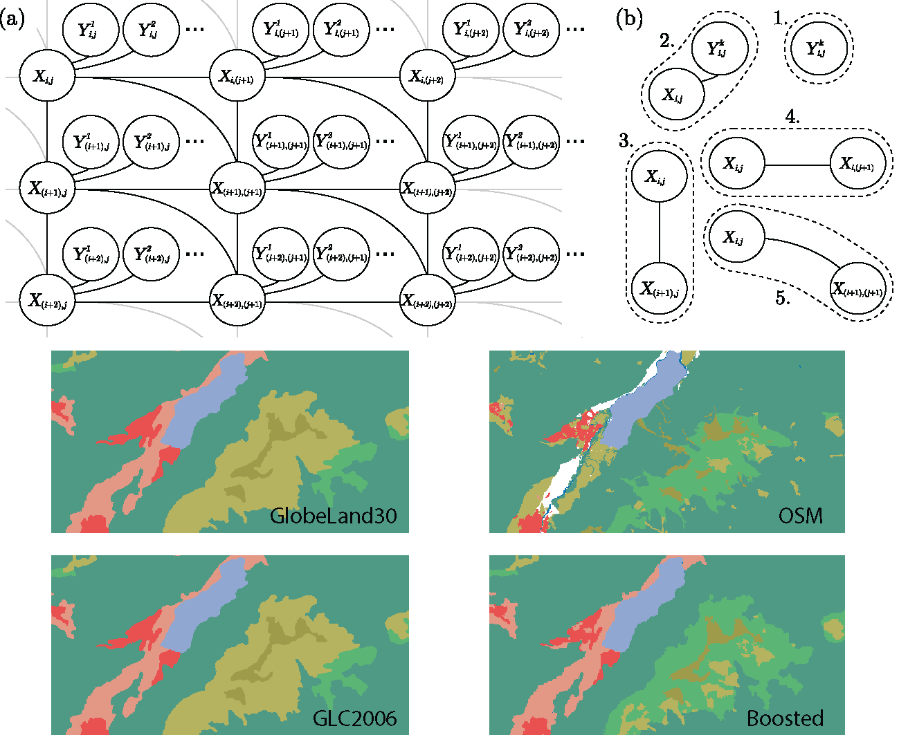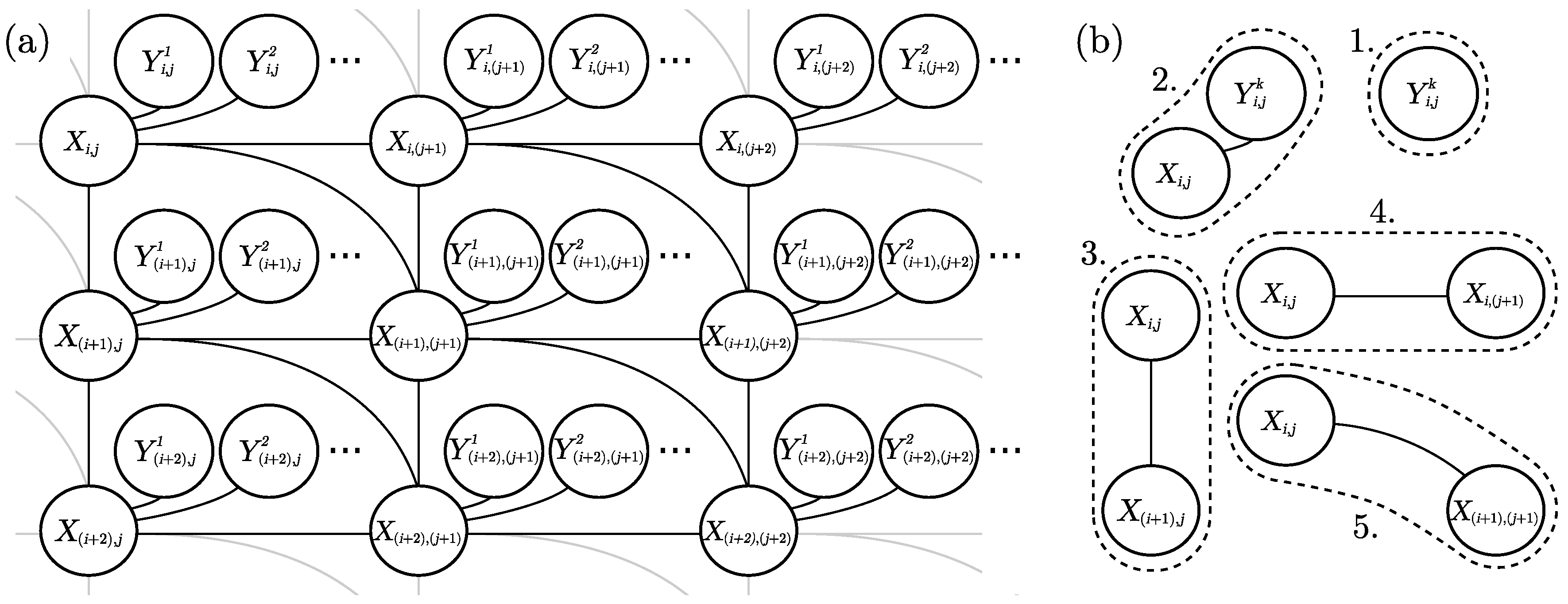Finally, we assign a relationship between all neighboring pixels of $X_{i,j}$ to enforce Tobler’s first law of geography. These variables and relationships are illustrated in Figure 1a.

For a PGM formulation of this model, we choose the factors in a manner that would capture the relationships of the model and can easily be initialized from the land cover data. This choice is outlined in Figure 1b and

Table 1. Factor setup for the land cover PGM.

	Num. of Factors	Factor Variables	Purpose
1.	$NMK$	$\{Y_{i,j}^k\}$	Capture the different classifications
2.	$NMK$	$\{Y_{i,j}^k,X_{i,j}\}$	Relationship between observations and underlying classes
3.	$(N-1)M$	$\{X_{i,j},X_{(i+1),j}\}$	Relationship between southward neighbors
4.	$N(M-1)$	$\{X_{i,j},X_{i,(j+1)}\}$	Relationship between eastward neighbors
5.	$(N-1)(M-1)$	$\{X_{i,j},X_{(i+1),(j+1)}\}$	Relationship between south-eastward neighbors

, along with a brief description of the purpose of each set of factors in the relationship model.

Our factors are then initialized according to the land cover classifications and assumptions in the form of expert knowledge. The idea is simple: we assign a discrete probability table to each factor according to an underlying relationship. More specifically, we set the observation variables $Y_{i,j}^k$ according to the land cover classification k: for hard classifications we have $p(Y_{i,j}^k={\mathrm{classification}}_{i,j}^k)=1$ and $p(Y_{i,j}^k\ne {\mathrm{classification}}_{i,j}^k)=0$, and for soft classifications we make use of joint probability tables initialized by expert knowledge about the likelihood of class co-occurrence in the defined region, and the class-specific classification quality, see

Table 2. Prior probabilities table of $P(X_{i,j},X_{i,(j+1)})$ for three classes a, b, and c, capturing expert knowledge. This is easily expandable to N classes, and the same table is usually applied to define relationship priors between eastward, southward and south-eastward neighbors.

	${\mathit{X}}_{\mathit{i},\mathit{j}}=\mathit{a}$	${\mathit{X}}_{\mathit{i},\mathit{j}}=\mathit{b}$	${\mathit{X}}_{\mathit{i},\mathit{j}}=\mathit{c}$
$X_{i,(j+1)}=a$	$P(a,a)$	$P(a,b)$	$P(a,c)$
$X_{i,(j+1)}=b$	$P(b,a)$	$P(b,b)$	$P(b,c)$
$X_{i,(j+1)}=c$	$P(c,a)$	$P(c,b)$	$P(c,c)$

. Furthermore, for the relational factors (such as Table 1 factors 2 to 5) the variables are more likely to have the same outcome.

Using our defined and initialized factors we (a) construct a cluster graph, (b) obtain a posterior distribution over this graph by means of PGM inference techniques and (c) extract the random variables $X_{i,j}$ from the posterior as the most likely land cover classifications. Thus, completing the boosting process by creating the boosted land cover classification using the $X_{i,j}$ variables.

A full discussion on the construction of a cluster graph, and PGM inference over the graph are beyond the scope of this paper. For this we refer the reader to in-depth literature on the topic such as Koller and Friedman [29]. However, a summarized overview of the construction, inference and settings used are presented below.

• Configuring a cluster graph correctly is not a trivial task and requires some heuristics. For the construction of our cluster graph we make use of the LTRIP procedure described by Streicher and du Preez [32].
• We used belief update, also known as the Lauritzen-Spiegelhalter algorithm [33] to perform inference over the graph.
• The convergence of the system, as well as the scheduling of messages, is determined according to the Kullbach-Leibler divergence between the newest and immediately preceding sepset beliefs.
• The distribution over a single variable $X_{i,j}$ is found by locating a factor containing the variable and then marginalizing out to that variable. For example, $P(X_{i,j})={\sum }_{Y_{i,j}}P(X_{i,j},Y_{i,j})$

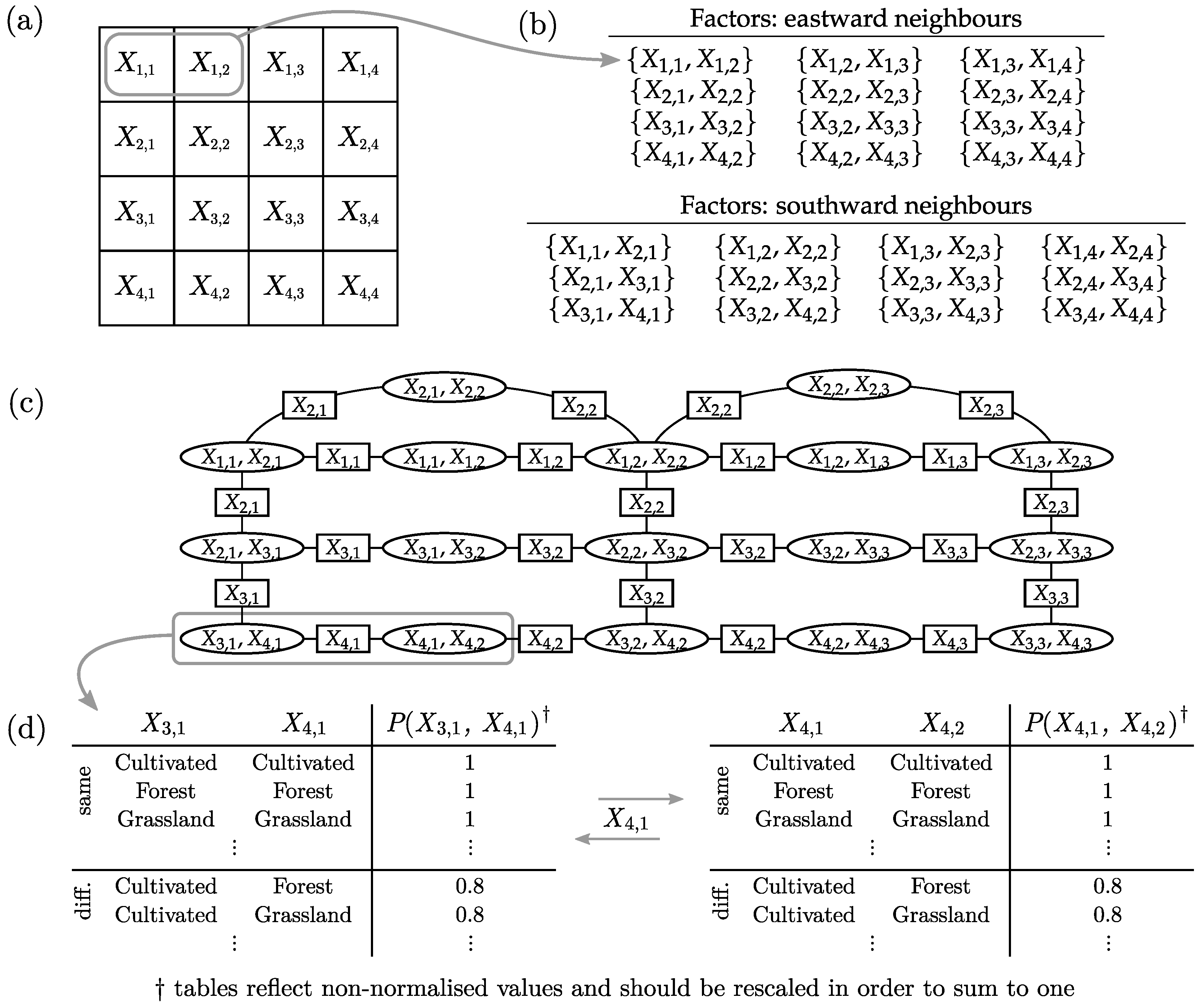
To better understand the proposed cluster graph architecture and inference process, see the reduced example presented in Figure 2. For illustrative purposes, we only consider the spatial factors (lines 3–5 of Table 1), we reduce the location grid to $4\times 4$ and use a constant probability to define all inter-class relationships. In practice the prior probabilities are to be specified by expert knowledge, and all factors need to be included to boost the original land cover datasets.

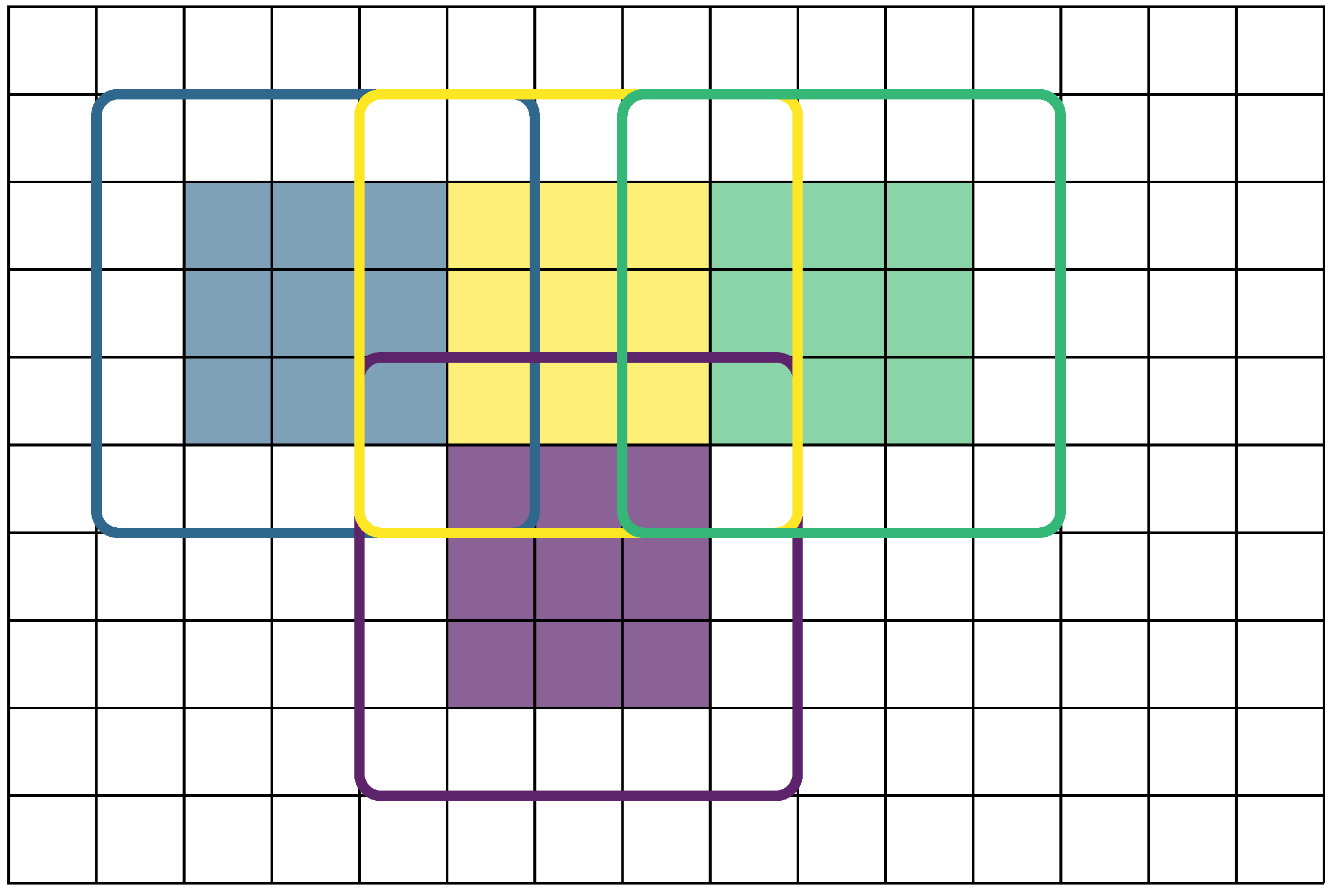
As a final note, since the number of factors grow by order $NM$, it is useful to split the problem up into smaller sections which can be processed in parallel. We found it safe to assume that regions sufficiently far apart have near-zero influence on each other from a factor point of view. Thus, we segmented the region into non-overlapping sub-regions, with an overlapping boundary to enforce smoothness along the edges. We then ran the cluster graph process on each of these sub-regions in parallel and finally stitched the posteriors together along the sub-region boundaries, while discarding the overlapping regions which may contain conflicting results. For a more intuitive understanding of this process, please refer to Figure 3.

3.3. Dataset

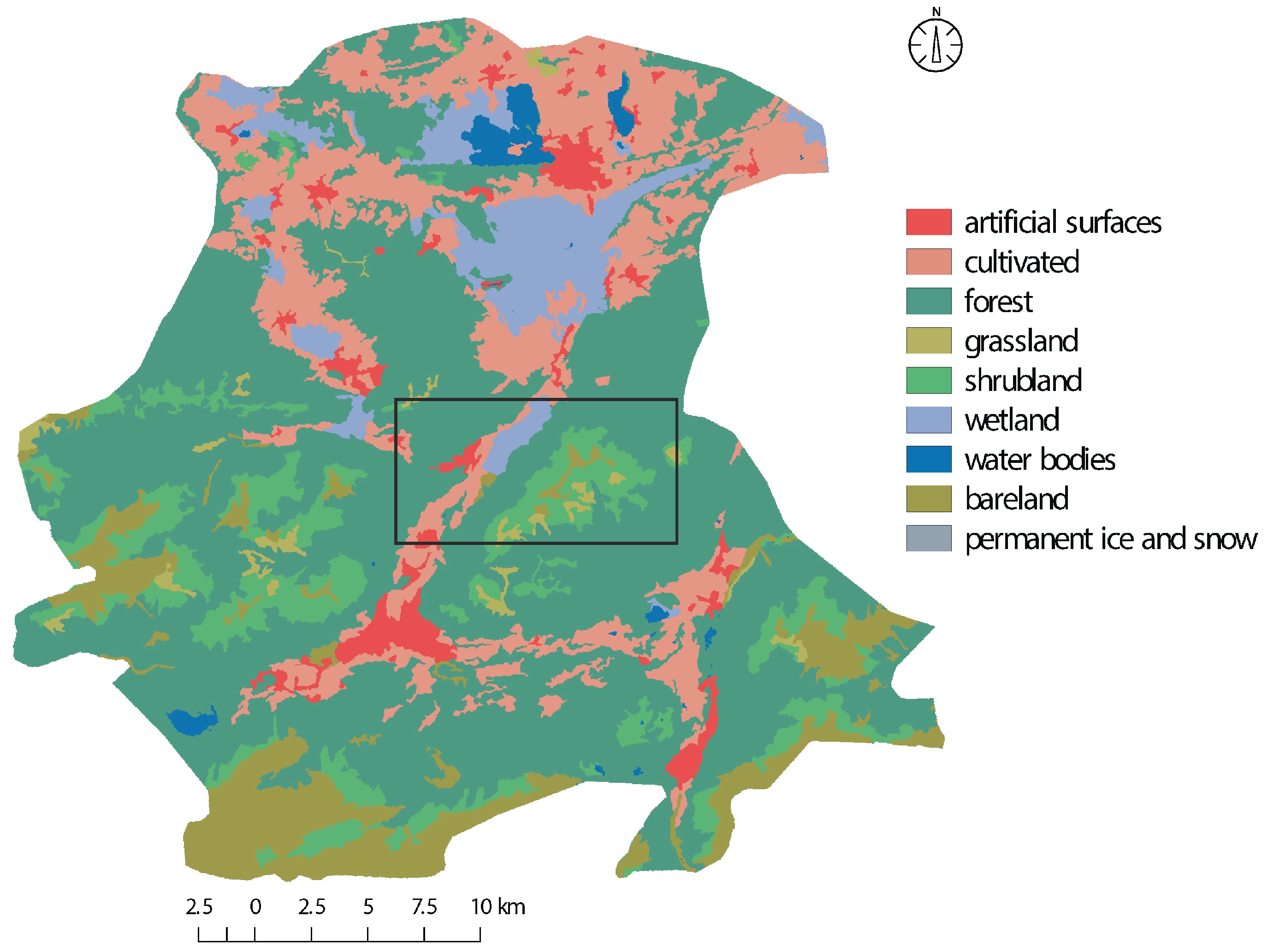
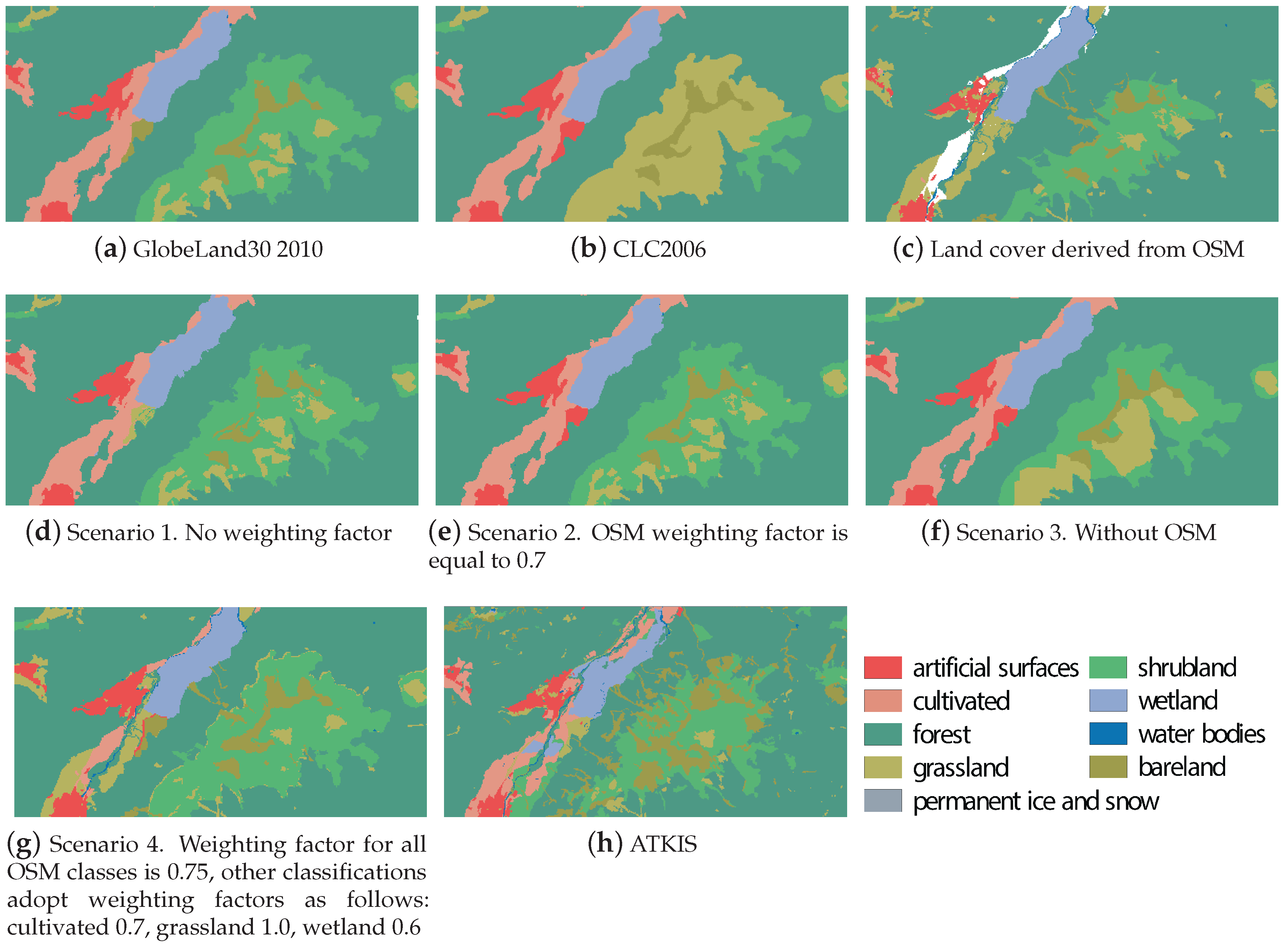
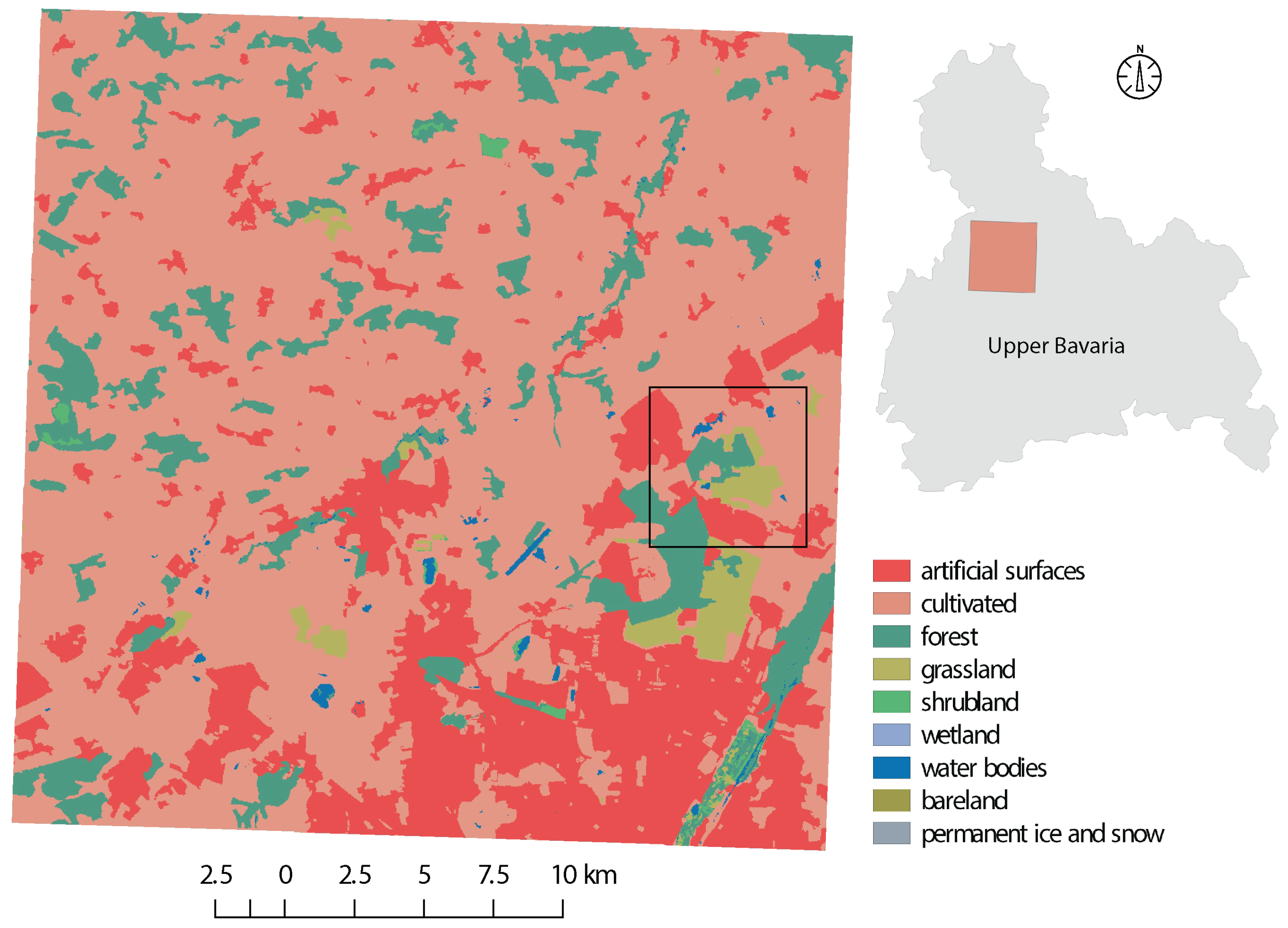
To assess our proposed approach, we selected two commonly used land cover datasets, namely GlobeLand30, CORINE Land Cover (CLC2006, Garmisch-Partenkirchen, Germany), and additionally land cover data derived from Volunteered Geographic Information (VGI) such as OpenStreetMap. The test region of Garmisch-Partenkirchen, Germany (101,224 km${}^2$) was selected due to the availability of high-quality data sets and sufficient diversity in the distribution of land classes. The land cover classifications are temporally independent of one another, each having been derived from imagery captured over different periods of time. While the temporal disparity between the datasets could cause problems in boosting applications, due to conflicting information caused by large temporal change events. The assumption was made that little temporal change has occurred over the dataset acquisition period, due to the nature of the test location. Thus, despite the temporal data heterogeneity, the benefit of the current work is seen in applying cluster graph approach for boosting land cover classifications.

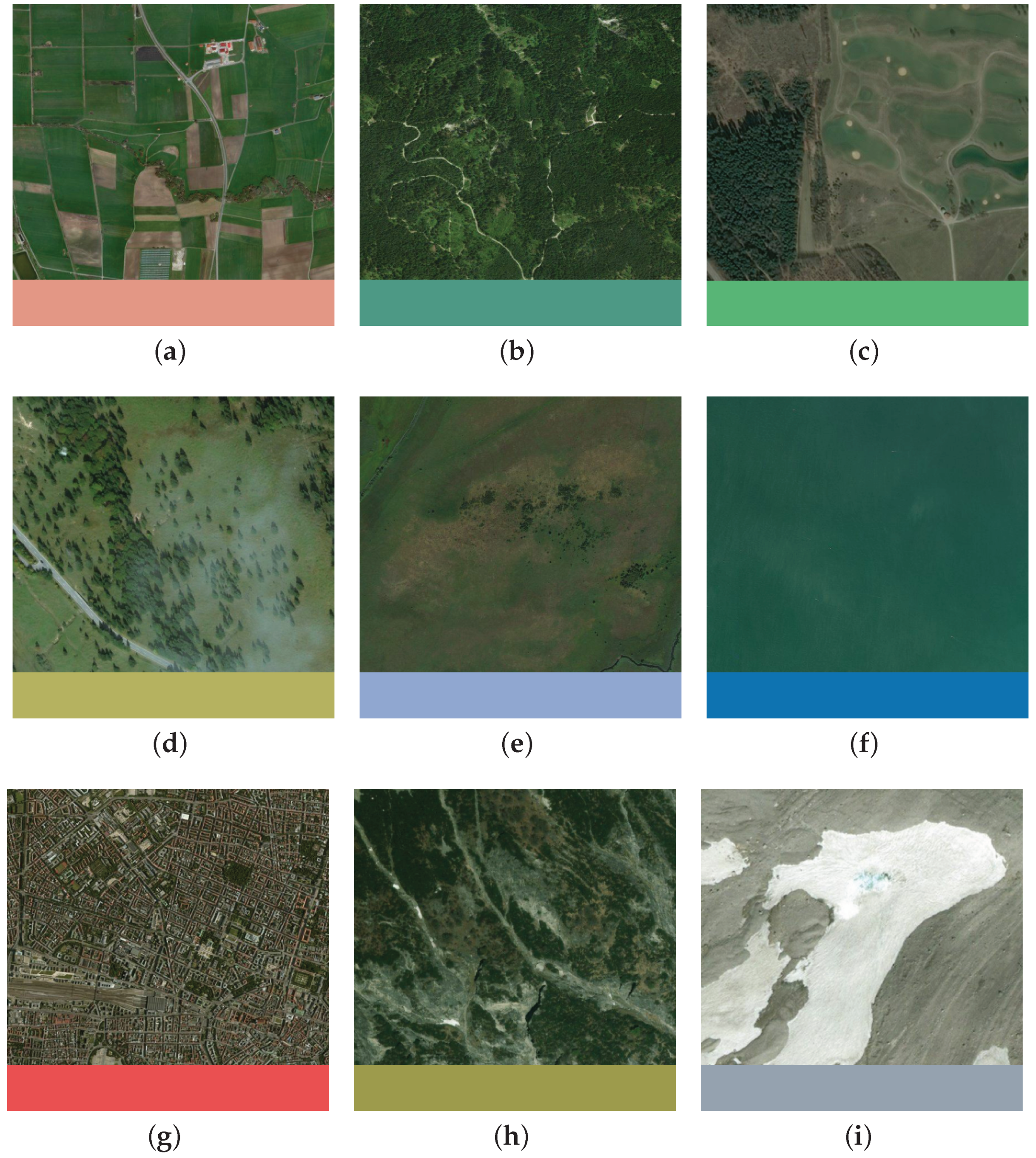
GlobeLand30 is a global scale land cover product of 30m resolution for two base-line years (2000 and 2010). For this study we make use of the 2010 version of the dataset. This dataset is comprised of 10 major land cover classes, namely cultivated areas, forests, grassland, shrubland, wetland, water bodies, tundra, artificial surfaces, bare land and permanent snow and ice. Although the GlobeLand30 dataset is comprised of 10 major classes, only 9 of these classes are present in our study region. The classes which are defined for our study area are depicted in Figure 4 with examples of the visual appearance of each class.

To reduce the effects of cloud cover on the creation of the GlobeLand30 dataset, the raw remote sensing imagery was selected to coincide with the local vegetation growth season [2]. Thus, the land cover classification was created based on mosaic of suitable images with minimal cloud occlusions. According to data provider, the land cover classifications of our study area were generated from a mosaic of images acquired on 31 August 2009. Previous studies indicate that the overall classification accuracy of GlobeLand30 can range from 46% [34] and up to 80% [2,35,36], and thus the true accuracy of the dataset is heterogeneous.

Land cover mapping that specifically focuses on the EU countries is realized within the CORINE (“Coordination of Information on the Environment”) program. The CLC2006 (CORINE Land Cover 2006) dataset for the area of Germany follows common European-wide CORINE Land Cover nomenclature that consists of 44 classes, where 37 classes are relevant for Germany and 29 classes are relevant for the study area. We scaled down the class complexity to provide consistent classification for all the data sources. This was achieved by reassigning the 44 CORINE land cover classes into the 10 classes provided by the GlobeLand30 classification. The details of the reclassification processes can be seen in

Table 3. Reclassification of CLC2006 land cover classes relevant for the study area based on the GlobeLand30 scheme.

Land Cover Classes	CLC2006, Pixel Values	GlobeLand30, Pixel Values
Cultivated	32–41	10
Forest	42–45	20
Grassland	46–47	30
Shrubland	48–49	40
Wetland	55–59	50
Water bodies	60–64	60
Tundra	-	70
Artificial surfaces	21–31	80
Bareland	50–53	90
Permanent ice and snow	54	100

.

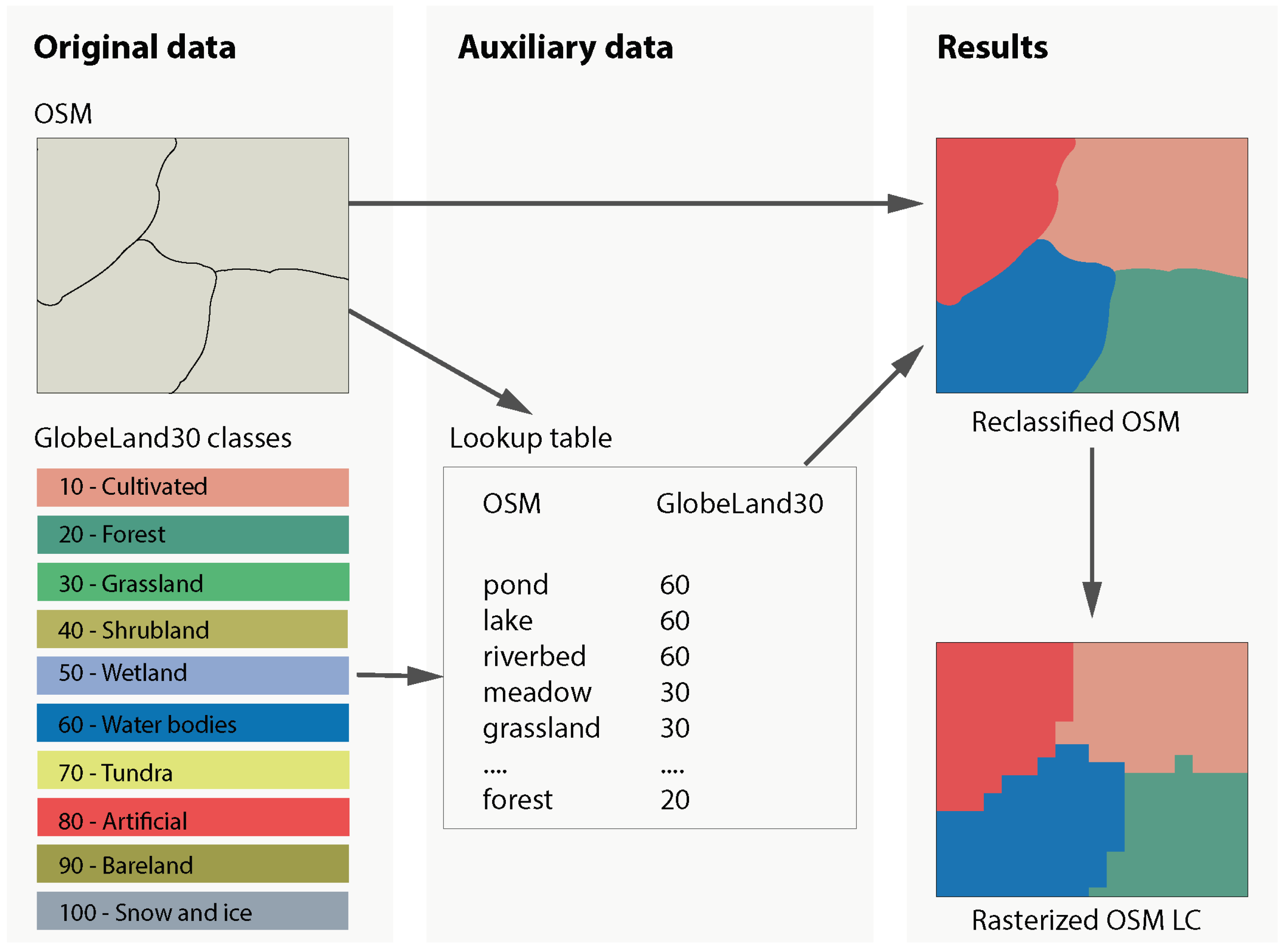
Along with GlobeLand30 and CORINE (CLC2006), data from OpenStreetMap (OSM) plays an important role in this study as an auxiliary source. The OSM (openstreetmap.org) is one of the most widespread and well-recognized VGI projects. Although the OSM data is not specifically tailored to the needs of land cover mapping and the OSM data and user community is very heterogeneous, the data has valuable input for the land cover classification. In our research, we implemented a method suggested by [37] for deriving a land cover map from the OSM database as shown in Figure 5. To preserve the entire content of the database, we use a complete XML-encoded extract of the OSM database, representing our study area, instead of pre-processed Shapefiles distributed by OSM data providers. The data pre-processing has been done in a combination of automatic and manual OSM tag annotations to GlobeLand30 classification scheme. For the derivation of the land cover map, a subset of the OSM tags, namely “amenity”, “building”, “historic”, “land use”, “leisure”, “natural”, “shop”, “tourism”, and “waterway” are considered. This mapping is only conducted for polygon features, since point and line features do not provide immediate information about the coverage of an area. We define a mapping from the OSM attributes to the classes used in the GlobeLand30 classification scheme.

The data is then rasterized and resampled using a nearest neighbor approach to generate a land cover classification with the same resolution and spatial alignment as the GlobeLand30 dataset. The workflow for converting the OSM data into a land cover raster product is depicted in Figure 5.

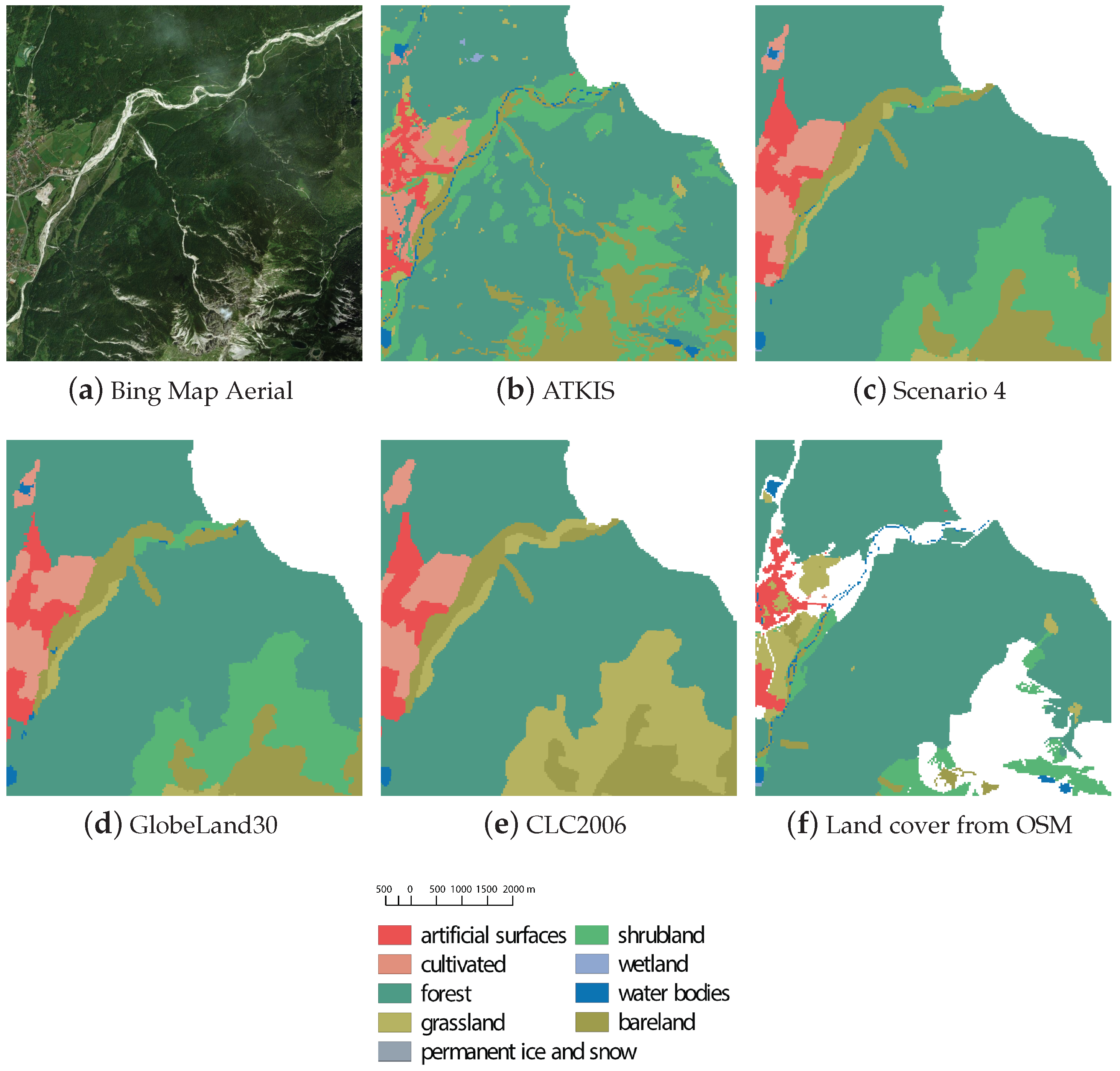
To accurately access our classification boosting approach a ground-truth dataset was required. As it is intractable to obtain a truly accurate land cover classification for the whole study area, and thus an accurate reference dataset, we chose to make use of a well maintained, and frequently updated, official land cover classification for this purpose. The national dataset called Amtliches Topographisch-Kartographisches Information System (ATKIS) was selected as the reference dataset for our investigation. This dataset represents a Digital Landscape Model of scale 1:10,000 and 1:25,000 (Basis-DLM), and was provided by an official national cartographic authority (Bundesamt für Kartographie und Geodäsie). Our selection was further motivated by the reported use of this dataset as a reference map by numerous other authors [36,38].

Dataset Pre-Processing

Pre-processing and harmonization of the classes among these three heterogeneous datasets was performed to simplify the construction of the cluster graph. However, it should be noted, that this step is not required and merely reduces the complexity in defining the inter-class relationships between the various datasets by ensuring a common set of class labels exist for all the datasets.

The details of our pre-processing steps are outlined below:

• All datasets are cropped to the municipal boundary of Garmisch-Partenkirchen;
• The classes of OSM and CLC2006 are normalized to match the 10 classes specified by GlobeLand30;
• The datasets were then rasterized with 30m pixel resolution and aligned to GlobeLand30 using the nearest neighbor re-sampling method as found in standard GIS software. This ensured that each pixel was covering the same area of land. For OSM data the process is more involved and is described in Figure 5.
• Individual rasters were then sub-divided into sub-regions as per the explanation in Section 3.2.

3.4. Definition of Priors and Parameters

In addition to the cluster graph implementation and dataset, our approach requires an inter-class joint probability table, a per map confidence factor as well as the definition of sub-region and boundary size.

The joint probability table is defined based on expert knowledge and fundamental laws of geography. Classes which are likely to occur next to each other are assigned to a high probability, while classes unlikely to neighbor each other—based on region, geography, and expert assumptions, are assigned a low value. The self-occurrence probability of each class $P(n,n)$ is assigned the highest value to add dependence on Tobler’s first law of geography. Due to the nature of inference in cluster graphs, and PGMs in general, the values defined in the prior joint probability table do not need to be exact probabilities, but rather need to reflect the relative relationships between various classes. For instance if $P(a,b)=P(a,c)$ and $P(a,b)>>P(a,d)$ this reflects that it is equally likely that class b or c could neighbor class a and that it is significantly less likely that class d would neighbor class a. The full joint probability table used in our experiments can be seen in

Table 4. Non-normalized joint probability table of inter-class relationships as defined by expert knowledge (To reflect true probabilities, the table must be rescaled to sum to one).

	Cultivated	Forest	Grassland	Shrubland	Wetland	Water	Artificial	Bareland	Snow
cultivated	1	0.15	0.4	0.05	0.2	0.05	0.4	0.05	0.05
forest	0.15	1	0.05	0.4	0.2	0.05	0.15	0.05	0.05
grassland	0.4	0.05	1	0.2	0.15	0.15	0.05	0.05	0.05
shrubland	0.05	0.4	0.2	1	0.15	0.05	0.05	0.15	0.05
wetland	0.2	0.2	0.15	0.15	1	0.4	0.05	0.05	0.05
water	0.05	0.05	0.15	0.05	0.4	1	0.05	0.2	0.05
artificial	0.4	0.15	0.05	0.05	0.05	0.05	1	0.2	0.05
bareland	0.05	0.05	0.05	0.15	0.05	0.2	0.2	1	0.65
snow	0.05	0.05	0.05	0.05	0.05	0.05	0.05	0.65	1

.

In addition to introducing expert knowledge into the inference process through the inter-class joint probability table, we also include further expert knowledge in the form of a classification map confidence factor. This factor can be used to weight the confidence in each of the input datasets as a whole, or in a class-wise manner, and the weighting factor can either be set by expert opinion or through more complex statistics.

To assess the effects of including VGI, in the form of OSM data, we performed multiple experiments where the confidence in the OSM data was adjusted according to expert opinion. The confidence factors for the CLC2006 and GlobeLand30 datasets were kept constant to only assess the effect of VGI data which is often an incomplete, and noisy source of land cover information.

The selected confidence factors are described in

Table 5. Land cover map confidence scores for adding prior information about dataset confidence, this data is captured by the observation factors $(Y_{i,j}^k,X_{i,j})$ in Table 1. Four scenarios were evaluated to determine the effects of various expert assumptions. * Scenario 4: The OSM layer confidence was not uniformly weighted per class, with cultivated = 0.7, grassland = 1, wetland = 0.6 and remaining classes = 0.75.

	Scenario 1	Scenario 2	Scenario 3	Scenario 4
GlobeLand30	1	1	1	1
CLC2006	1	1	1	1
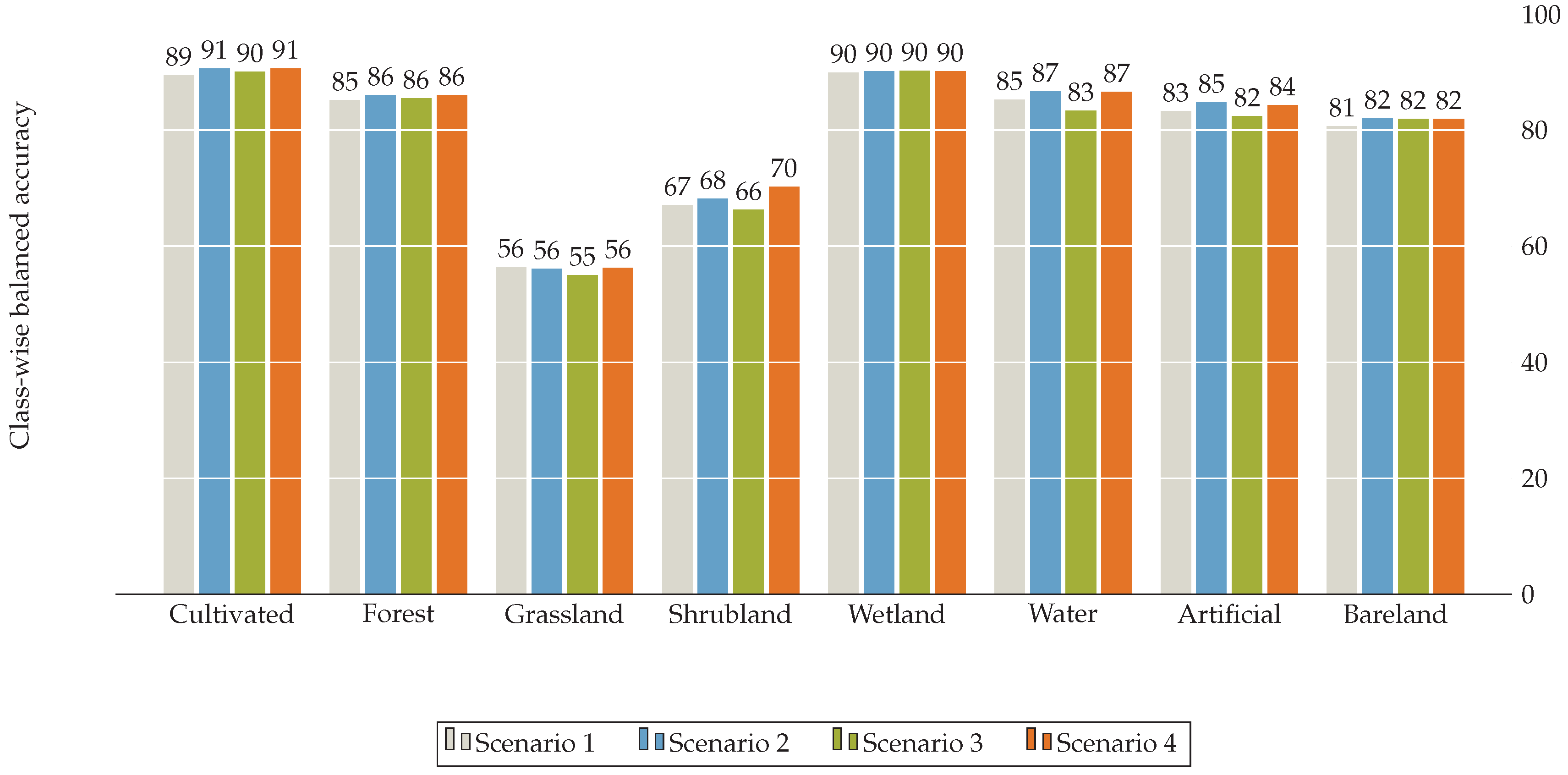
OSM	1	0.7	0	0.75 *

and each of our experimental setups are detailed below:

• Scenario 1: All land cover maps were assumed to be of equal quality ($p(Y_{i,j}^k=\mathrm{Classification})=1$).
• Scenario 2: OSM data was assumed to be less accurate overall ($p(Y_{i,j}^{\mathrm{OSM}}=\mathrm{Classification})=0.7$).
• Scenario 3: OSM data was excluded completely from the boosting process ($p(Y_{i,j}^{\mathrm{OSM}}=\mathrm{Classification})=0$).
• Scenario 4: OSM data is assumed to be less accurate overall, except for grassland. The classes are weighted as follows: overall OSM weighting: 0.75, cultivated: 0.7, wetland: 0.6 and grassland: 1.0.

Lastly, the size of the sub-regions and boundaries was defined such that each sub-region was square with a side length of $35px$ (1050 m) and a boundary of $6px$ (180 m). It was found that a total boundary width (left + right, or top + bottom) which is between 25% and 50% of the sub-region width or length is appropriately large that the edge factors have a negligible influence. In our case our boundary was defined as $\frac{12px}{35px}\approx 35\%$.

4. Results

In this section, we report on the results obtained using our cluster graph land cover boosting approach. We assess the accuracy of the land cover maps produced and evaluate the uncertainty (in the form of the Shannon diversity index) extracted during classification boosting process. To perform our assessments, we make use of the dataset defined in Section 3.3 over the study area of Garmisch-Partenkirchen, Germany (see Figure 6). To perform an assessment of thematic classification accuracy, we adopted the method of error matrix and provide accuracy metrics such as the overall accuracy, Kappa, and the class-wise balanced accuracy.

The overall accuracy represents the proportion of correctly classified pixels to the reference map. The Kappa coefficient [−1, 1] indicates how well the classification performed when it is compared to randomly assigned values. In other words, the Kappa values can represent an agreement between two classifications, where values less than 0 show no agreement, values 0.0–0.4 represent a small degree of agreement, values between 0.41 and 0.61 represents moderate agreement, values 0.41–0.61 indicate significant agreement, and values 0.81–1 show strong agreement. Furthermore, we use the class-wise balanced accuracy [39] to evaluate the classification on a class-wise basis. The class-wise balanced accuracy represents correctly classified proportions for each class, which is essential as the classes are imbalanced in their distribution within the scene. This measure is favored over the traditional consumer, producer accuracy as we are making comparison to a reference dataset rather than to true ground-truth data. Thus, the class-wise balanced accuracy represents both the consumer and producer accuracy as a single accuracy measure which is weighted according to the class distribution in the reference dataset.

To quantitatively assess the accuracy of our boosted land cover maps we compare our boosted land cover classifications against a reference land cover mapping. As reference we chose to use a national dataset called ATKIS which represents a Digital Landscape Model of scale 1:250,000 (Basis-DLM) provided by an official cartographic authority (Bundesamt für Kartographie und Geodäsie). The remainder of the classification and uncertainty results are analyzed in a qualitative manner with respect to the individual land cover classifications used as input to our proposed cluster graph.

4.1. Effect of Prior Information

To assess the effects of expert knowledge and the inclusion of VGI, we tested four different scenarios. In all the scenarios the initial inter-class priors were assigned according to Table 4; however, the overall confidence factor for each dataset was altered on a global and class level as described in Table 5 and further in Section 3.4.

Using these expert beliefs, we performed inference over the test region and compared the final boosted classification to the ATKIS dataset to determine the effects of various sets of expert knowledge an VGI on the final boosted classification. The results of these comparisons can be seen in Figure 7 with a more detailed analysis of overall accuracy and Kappa in

Table 6. Overall accuracy and Kappa results of various test scenarios with respect to ATKIS reference dataset.

Estimate	Scenario 1	Scenario 2	Scenario 3	Scenario 4
Accuracy	0.7741	0.7798	0.7648	0.7828
Kappa	0.6581	0.6704	0.6506	0.6748

.

4.2. Qualitative Assessment of Scenarios

We further investigate the various scenarios in a qualitative manner by evaluating the final boosted land cover maps. Figure 8 shows a subsection of our study area for each of our four test scenarios, as well as for the input and reference data. Using this approach, we can gain a visual understanding and intuition for the performance of our approach.

4.3. Comparison to Individual Datasets

From Figure 7 and Table 6 it is clear that Scenario 4, with class-wise weighting, appears to provide the best results. For this reason, we will use Scenario 4 as the output from our approach to compare to the performance of the original land cover classifications of CLC2006, OSM and GlobeLand30.

Comparing the classifications to the ATKIS dataset we obtain class-wise accuracy as depicted in Figure 9 with an overall accuracy for the various land cover classifications as described in

Table 7. Accuracy assessment and comparison of the original datasets to the approach proposed.

Estimate	CLC2006	OSM	GlobeLand30	Scenario 4
Accuracy	0.7452	0.7405	0.7697	0.7828
Kappa	0.6228	0.5013	0.6564	0.6748

.

As it has been mentioned, the overall accuracy represents the proportion of correctly classified pixels to the reference map. For this reason, the measure of accuracy is relative rather than absolute, as it depends on the quality of the reference data [40]. In our case the ATKIS dataset provides a larger variety of classes and more detailed coverage than the datasets which we are boosting, and thus the overall accuracy is relative to the level of detail on the reference map. The relative nature of the accuracy is an important factor to keep in mind when assessing the results with respect to existing work which might employ another reference map, or accuracy measure.

Additionally, we compare the prior land cover classifications and our best boosted classification to an aerial image and the ATKIS reference data in Figure 10. From this figure the heterogeneity of the datasets, and the incomplete nature of the OSM dataset is clearly visible.

4.4. Classification Uncertainty

Due to the Bayesian framework which cluster graphs are rooted in, we obtain a measure of the probability for the likelihood of each class being present in each pixel of the boosted land cover map. Based on these probabilities we can extract an uncertainty metric, Shannon diversity index, for each pixel in our boosted land cover classification map.

The uncertainty map for our approach (Scenario 4), and a zoomed in section corresponding to the boosted region depicted in Figure 10, is depicted in Figure 11.

4.5. Validation Study

Unlike machine learning methods, Bayesian methods do not typically require an independent validation study as there is no differentiation between training and testing phases. However, to assess the validity of the assumptions we made in defining factors and priors, as well as our approaches ability to generalize to other regions, we performed a validation study. This study was conducted by applying the proposed cluster graph approach to an auxiliary study area, of 84,850 km${}^2$, within Germany (see Figure 12). To evaluate the generalization of our approach with respect to the setting of priors and confidence factors, we kept these values as they were defined for the original test region (Scenario 4).

The validation study represents six land cover classes with largest coverage for artificial and agricultural area. By applying the same approach, we were able to produce a boosted land cover classification with the overall accuracy given in

Table 8. Validation study: Accuracy assessment and comparison of the original datasets to the approach proposed.

Estimate	CLC2006	OSM	GlobeLand30	Our Approach
Accuracy	0.8302	0.8009	0.8401	0.8434
Kappa	0.6952	0.6886	0.7054	0.7111

. Figure 13 introduces a comparison of different land cover datasets over the validation area.

5. Discussion

Generally, the results presented in Section 4 show that our boosting method can merge existing land cover classifications in a robust manner. Furthermore, it shows that we can generate an accurate uncertainty map of the boosted area, which is useful in analysis of the boosted land cover map.

In this section, we further investigate these results and describe the capabilities and advantages of our method for land cover boosting, as well as describe its short falls.

5.1. Comments on the Effect of Priors

As priors are set based on expert knowledge, and are therefore subjective by nature, it is difficult to fully analyze the effect of various decisions on the accuracy. However, we can make a few key observations based on the results we presented. From Figure 7, we can see that all scenarios which include all the datasets have a similar accuracy, while Scenario 3 which excludes OSM data all together has a slightly lower accuracy across many classes. However, the accuracy measure does not provide a complete picture about how this factor affects the overall boosted classification appearance. From Figure 8 we can see that the overall map confidence factor does not significantly change the final boosted classification, while class-wise confidence factors have a somewhat larger effect on the final booster classification (See Figure 8d,e,g). By adapting class-wise confidence factors of the VGI dataset, we can better capture fine details which are well represented in human labeled datasets (such as river and water features). These types of features are usually only present in land cover maps created with a relatively small minimum mapping unit, and thus are often not represented by existing large-scale land cover datasets such as GlobeLand30 and CLC2006.

Table 6 confirms that the inclusion of more detailed prior information leads to a better overall accuracy, with a greater Kappa coefficient. However, the overall differences are relatively small, and thus it can also be interpreted that the proposed cluster graph approach is robust to the setting of priors and can produce an overall accurate boosted classification for a range of prior configurations. This is likely due to the strong inference abilities of cluster graphs which allow this approach to determine the complex inter-dependencies between factors. This coupled with our geographically centered design approach appears to capture the most important relationships and thus forgoes the need for strong expert priors to generate a reasonable land cover classification.

Apart from the effect of priors, Table 6, reveals that the inclusion of VGI has a positive effect on the overall accuracy of the final boosted classification. Thus, it can be said that the inclusion of additional datasets, even if noisy and incomplete, plays a larger role on the overall accuracy than the configuration of priors.

5.2. Qualitative View of Boosted Classification Accuracy

Taking a purely qualitative approach we compared the boosted classifications from our test scenarios over a diverse subsection of our study area. In Figure 8, we can see the classification differences between our four test scenarios, the original land cover classifications and the ATKIS reference datum.

Based on Figure 8 it is clear how the inclusion of various datum, as well as the selection of priors affect the overall boosting process. Furthermore, we can observe how our approach preserves spatial consistency between neighboring classes even when the input data sources are noisy, conflicting, or incomplete. This observation is particularly clear in Scenario 4 (Figure 8g) where the river feature from the OSM dataset is included in the boosted classification, but the area around this feature remains spatially consistent with the information presented by CLC2006 and GlobeLand30.

Figure 10 depicts another sub-region of our test scene. The ability of our approach to perform reasonable inference in the presence of conflicting and missing data becomes clear. The lower right area of the region has very sparse coverage in the OSM dataset, and conflicting labels in the GlobeLand30 and CLC2006 datasets. In this case, our approach can infer a suitable and accurate (with comparison to ATKIS and the aerial image) land cover mapping, while still maintaining smaller features, such as lakes and grassland areas, and spatial consistency (smooth land cover mapping, and reasonable neighboring classes). Additionally, by referring to the produced land cover uncertainty map for this region, Figure 11, it is clear that the areas where land cover was inferred based on missing, and conflicting evidence show higher uncertainty than areas where all three input data sources agreed. Thus, our cluster graph approach can be said to be reasoning in a rational manner.

Furthermore, the results of our validation study, Figure 13, once again show how spatial consistency is preserved, and how even in the presence of noisy VGI and conflicting information our cluster graph approach can boost the classifications to generate a detailed land cover classification. One particular area of interest is the area between the forest, artificial and cultivated classes to the left of the center of the image. In this region the OSM data is incomplete, and the CLC2006 and GlobeLand30 classifications are conflicting. However, even in the presence of this our boosting approach can infer a classification for this region in a spatially consistent manner. While the classification for the region in CLC2006 is grassland, and in GlobeLand30 is artificial, our boosted classification labels the area as cultivated. This labeling is likely the result of the strong preference for preserving Tobler’s first law of geography, as well as prior about inter-class relationships. Upon inspection of the aerial image of this region, it can be seen that while our classification overlooks a small artificial region, the remainder of the classification is feasible.

While our approach does lose some granularity in smaller spatial areas, this could be considered a reasonable trade-off, given that some of the finer features are not present in more than one of the input data sources. Additionally, this smoothing effect could possibly be a consequence of the patch-based processing approach we employed, as detailed in Figure 3.

5.3. Quantitative View of Boosted Classification Accuracy

Making reference to the overall accuracy of our approach on the test and validation study areas, Table 7 and Table 8, it can be seen that our boosted land cover classification exhibits the highest overall accuracy when compared to our ATKIS reference dataset. Furthermore, the Kappa coefficient of our land cover classification is significantly higher in both cases. In general, our approach far exceeds the accuracy of OSM and CLC2006 land cover and has a small improvement over GlobeLand30. As overall accuracy does not provide a complete picture of land cover classification accuracy we further investigate and analyze the balanced class-wise accuracy of the prior data and our boosted classification.

Based on the respective balanced, class-wise accuracy of our test scene, as depicted in Figure 9, it can be seen that our approach shows reasonable performance in all classes. While the accuracy of OSM does exceed our approach for some classes, it should be noted that our approach is never affected by poor class accuracy in any of the datasets. For instance, with respect to bareland, shrubland and cultivated classes, the accuracy of our approach is always better or on par with the other sets of input data. This property could be argued to be of more significance than being able to always achieve the best accuracy in each class. The reason for this is that our approach can perform at a consistent level, even in the presence of noisy input data, and thus can provide a higher quality overall land cover classification.

By examining the class-wise accuracy for our validation scene, Figure 14, the same observations can be made. While in the validation scene OSM performs the best overall, it should be noted that the confidence factor for the OSM dataset was not adjusted, and thus the evidence from the OSM dataset was down weighted in the cluster graph. However, even with this low confidence in OSM, our approach was still able to extract value from the high accuracy OSM data to improve its results accuracy over CLC2006 and GlobeLand30. This once again showing the robustness of a cluster graph approach in the presence of ill-defined priors. As the OSM dataset for this region is significantly less sparse than for our test region, the confidence factor should have been adjusted upwards. Furthermore, the region contains large areas of cultivated land, which is known to be a source of conflict among CLC2006 and GlobeLand30 and thus expert knowledge should have been used to adjust the confidence factors and priors for the region, prior to boosting the land cover classification.

While class accuracy does not depict a large improvement over existing methods, the power of our proposed approach is in its ability to select and fuse the existing approaches in such a way as to have an overall better land cover classification than each of the individual land cover maps which were boosted. Furthermore, our approach can perform boosting in the presence of noisy, incomplete, and conflicting input data, while preserving spatial consistency and producing an overall reasonable, detailed and still diverse land cover classification.

5.4. Comments on Classification Uncertainty

Perhaps one of the largest benefits of the proposed approach is that it provides us the probability for each class occurring at each pixel. These class-wise probabilities can easily be exploited to generate uncertainty maps of the boosted land cover classification as well as for the original datasets. Due to the nature of the aerial imagery which is often used to generate land cover classifications, there are inherent inter-class ambiguities which exist due to the lack of height information. The generated uncertainty maps can help develop better algorithms for classification of land cover by either forming part of the optimization function, or by providing experts with clues as to which areas are often misclassified and why.

By comparing the uncertainty map, Figure 11, to the corresponding classification maps, Figure 10, it is clear that the uncertainty for each region tends to agree with intuition about the nature of certainty across the datasets. Regions which present conflicting information in two inputs and are missing information in the third are deemed to be more uncertain in the boosted map, while areas with agreement present a very low uncertainty. Perhaps one interesting observation is the low uncertainty in some regions where information is conflicting, this is likely due to the expert priors which enforce self-similarity based on Tobler’s law of geography.

Uncertainty maps can provide useful inputs into ecological and climactic research where uncertainty about land cover classifications can help improve models of land use dynamics and ecosystem stability. Furthermore, the class-wise probabilities could open the door for manual intervention where the top-n classes which exhibit similar probabilities could be presented to practitioners for disambiguation and thus further improvement of the overall land cover map. This process could further be expanded to fine tune the inter-class priors and thus improve the overall performance of the proposed approach.

6. Conclusions

In this paper, we presented a PGM approach to boosting of land cover classification maps. The formulation of the proposed solution took the form of a cluster graph which used observation and relational factors, along with expert knowledge to perform inference across multiple existing land cover classification data products. The study is applied to land cover classifications derived from remote sensing data, as they are among of the crucial inputs to environmental analysis that supports research on topics such as climate change, deforestation, urban change, and population growth. Additionally, we made use of incomplete, but accurate VGI, namely OpenStreetMap (OSM), as an additional set of evidence for land cover classification boosting. Furthermore, we analyzed how confidence factors could be used to benefit from accurately labeled regions of data, while reducing the effect of inaccurate and incomplete areas on boosting.

Our approach exploits existing expert knowledge, as well as constraints such as Tobler’s first law of geography, to improve the accuracy of land cover classification in the study region of Garmisch-Partenkirchen, Germany. Taking expert knowledge into account enables a classification boosting process with more flexibility and robustness. This approach allows for practitioners to customize the tool to their needs, while still being robust enough to compensate for poor assumptions and/or initialization.

Using the cluster graph approach, we were able to produce a feasible, diverse, and spatially consistent boosted land cover classification, based on GlobeLand30, CLC2006 and OSM data. Our boosted classification exhibited an overall accuracy improvement of around 1.4% when compared against a reference land cover classification map of our test region. Furthermore, our approach was applied to a validation region without adjustment of the priors and was shown to perform well even when initialized with a sub-optimal set of priors.

In addition to producing accurate boosted land cover classifications, the proposed approach can provide additional information on the uncertainty of the boosted classification as well as highlight commonly misclassified classes within our study region. These additional products are not available when using naive boosting methods or learned ensemble methods and can provide important insights into better understanding land cover and land use dynamics.

References

1. Arino, O.; Ramos Perez, J.J.; Kalogirou, V.; Bontemps, S.; Defourny, P.; Van Bogaert, E. Global Land Cover Map for 2009 (GlobCover 2009). PANGAEA 2012. [Google Scholar] [CrossRef]
2. Chen, J.; Chen, J.; Liao, A.; Cao, X.; Chen, L.; Chen, X.; He, C.; Han, G.; Peng, S.; Lu, M.; et al. Global Land Cover Mapping at 30 m Resolution: A POK-Based Operational Approach. ISPRS J. Photogramm. Remote Sens. 2015, 103, 7–27. [Google Scholar] [CrossRef]
3. Giri, C.; Pengra, B.; Long, J.; LoveLand, T.R. Next Generation of Global Land Cover Characterization, Mapping, and Monitoring. Int. J. Appl. Earth Obs. Geoinf. 2013, 25, 30–37. [Google Scholar] [CrossRef]
4. Ban, Y.; Gong, P.; Giri, C. Global Land Cover Mapping Using Earth Observation Satellite Data: Recent Progresses and Challenges. ISPRS J. Photogramm. Remote Sens. 2015, 103, 1–6. [Google Scholar] [CrossRef]
5. Chen, J.; Dowman, I.; Li, S.; Li, Z.; Madden, M.; Mills, J.; Paparoditis, N.; Rottensteiner, F.; Sester, M.; Toth, C.; Trinder, J.; Heipke, C. Information from Imagery: ISPRS Scientific Vision and Research Agenda. ISPRS J. Photogramm. Remote Sens. 2015, 115, 3–21. [Google Scholar] [CrossRef]
6. Martino, L.; Fritz, M. New Insight into Land Cover and Land Use in Europe. Statistics in Focus. 2008. Available online: http://edz.bib.uni-mannheim.de/www-edz/pdf/statinf/08/KS-SF-08-033-EN.pdf (accessed on 7 January 2019).
7. Foody, G.M. Status of Land Cover Classification Accuracy Assessment. Remote Sens. Environ. 2002, 80, 185–201. [Google Scholar] [CrossRef]
8. Gislason, P.O.; Benediktsson, J.A.; Sveinsson, J.R. Random forests for Land Cover Classification. Pattern Recognit. Lett. 2006, 27, 294–300. [Google Scholar] [CrossRef]
9. Pal, M.; Mather, P. Support Vector Machines for Classification in Remote Sensing. Int. J. Remote Sens. 2005, 26, 1007–1011. [Google Scholar] [CrossRef]
10. Rußwurm, M.; Körner, M. Multi-Temporal Land Cover Classification with Sequential Recurrent Encoders. ISPRS Int. J. Geo-Inf. 2018, 7, 129. [Google Scholar] [CrossRef]
11. Fritz, S.; McCallum, I.; Schill, C.; Perger, C.; Grillmayer, R.; Achard, F.; Kraxner, F.; Obersteiner, M. Geo-Wiki.Org: The Use of Crowdsourcing to Improve Global Land Cover. Remote Sens. 2009, 1, 345–354. [Google Scholar] [CrossRef] [Green Version]
12. Pérez-Hoyos, A.; García-Haro, F.; San-Miguel-Ayanz, J. A Methodology to Generate a Synergetic Land-Cover Map by Fusion of Different Land-Cover Products. Int. J. Appl. Earth Obs. Geoinf. 2012, 19, 72–87. [Google Scholar] [CrossRef]
13. Gengler, S.; Bogaert, P. Integrating Crowdsourced Data with a Land Cover Product: A Bayesian Data Fusion Approach. Remote Sens. 2016, 8, 545. [Google Scholar] [CrossRef]
14. Chen, B.; Huang, B.; Xu, B. Multi-Source Remotely Sensed Data Fusion for Improving Land Cover Classification. ISPRS J. Photogramm. Remote Sens. 2017, 124, 27–39. [Google Scholar] [CrossRef]
15. Pal, M.; Mather, P.M. An Assessment of the Effectiveness of Decision Tree Methods for Land Cover Classification. Remote Sens. Environ. 2003, 86, 554–565. [Google Scholar] [CrossRef]
16. Shao, Y.; Lunetta, R.S. Comparison of Support Vector Machine, Neural Network, and CART Algorithms for the Land-Cover Classification using Limited Training Data Points. ISPRS J. Photogramm. Remote Sens. 2012, 70, 78–87. [Google Scholar] [CrossRef]
17. Huang, C.; Davis, L.; Townshend, J. An Assessment of Support Vector Machines for Land Cover Classification. Int. J. Remote Sens. 2002, 23, 725–749. [Google Scholar] [CrossRef]
18. Krizhevsky, A.; Sutskever, I.; Hinton, G.E. Imagenet Classification with Deep Convolutional Neural Networks. Adv. Neural Inf. Process. Syst. 2012, 25, 1097–1105. [Google Scholar] [CrossRef]
19. Marmanis, D.; Datcu, M.; Esch, T.; Stilla, U. Deep Learning Earth Observation Classification using ImageNet Pretrained Networks. IEEE Geosci. Remote Sens. Lett. 2016, 13, 105–109. [Google Scholar] [CrossRef]
20. Kussul, N.; Lavreniuk, M.; Skakun, S.; Shelestov, A. Deep Learning Classification of Land Cover and Crop Types using Remote Sensing Data. IEEE Geosci. Remote Sens. Lett. 2017, 14, 778–782. [Google Scholar] [CrossRef]
21. Castelluccio, M.; Poggi, G.; Sansone, C.; Verdoliva, L. Land Use Classification in Remote Sensing Images by Convolutional Neural Networks. arXiv, 2015; arXiv:1508.00092. [Google Scholar]
22. El-Deen Taha, L.G. Classifier Ensemble for Improving Land Cover Classification. Int. J. Circuits Syst. Signal Process. 2016, 10, 346. [Google Scholar]
23. Griethe, H.; Schumann, H. The Visualization of Uncertain Data: Methods and Problems. 2006. Available online: https://www.researchgate.net/publication/216756553 (accessed on 10 January 2019).
24. Jost, L. Entropy and Diversity. Oikos 2006, 113, 363–375. [Google Scholar] [CrossRef]
25. Correa, C.D.; Chan, Y.H.; Kwan-Liu, M. A Framework for Uncertainty-Aware Visual Analytics. In Proceedings of the VAST 09—IEEE Symposium on Visual Analytics Science and Technology, Atlantic City, NJ, USA, 12–13 October 2009; pp. 51–58. [Google Scholar] [CrossRef]
26. Zhang, L.; Ji, Q. Image Segmentation with a Unified Graphical Model. IEEE Trans. Pattern Anal. Mach. Intell. 2010, 32, 1406–1425. [Google Scholar] [CrossRef] [PubMed] [Green Version]
27. Bishop, C.M. Pattern Recognition and Machine Learning (Information Science and Statistics); Springer: Berlin/Heidelberg, Germany, 2006. [Google Scholar]
28. Schiele, B. Lecture Notes in Probabilistic Graphical Models and Their Applications. 2017. Available online: https://www.mpi-inf.mpg.de/fileadmin/inf/d2/GM/2017/gm-2017-1120-imageprocessing.pdf (accessed on 9 January 2019).
29. Koller, D.; Friedman, N. Probabilistic Graphical Models: Principles and Techniques, 1st ed.; MIT Press: Cambridge, MA, USA, 2009. [Google Scholar]
30. Ghimire, B.; Rogan, J.; Galiano, V.R.; Panday, P.; Neeti, N. An Evaluation of Bagging, Boosting, and Random Forests for Land-Cover Classification in Cape Cod, Massachusetts, USA. GISci. Remote Sens. 2012, 49, 623–643. [Google Scholar] [CrossRef]
31. Tobler, W.R. A Computer Movie Simulating Urban Growth in the Detroit Region. Econ. Geogr. 1970, 46, 234–240. [Google Scholar] [CrossRef]
32. Streicher, S.; du Preez, J. Graph Coloring: Comparing Cluster Graphs to Factor Graphs. In Proceedings of the ACM Multimedia 2017 Workshop on South African Academic Participation—SAWACMMM ’17, Mountain View, CA, USA, 23 October 2017; ACM: New York, NY, USA, 2017; pp. 35–42. [Google Scholar] [CrossRef]
33. Lauritzen, S.L.; Spiegelhalter, D.J. Local Computations with Probabilities on Graphical Structures and their Application to Expert Systems. J. Royal Stat. Soc. Ser. B Methodol. 1988, 50, 157–224. [Google Scholar] [CrossRef]
34. Sun, B.; Chen, X.; Zhou, Q. Uncertainty Assessment of GlobeLand30 Land Cover Data Set over Central Asia. ISPRS Int. Arch. Photogramm. Remote Sens. Spatial Inf. Sci. 2016, XLI-B8, 1313–1317. [Google Scholar] [CrossRef]
35. Brovelli, M.; Molinari, M.; Hussein, E.; Chen, J.; Li, R. The First Comprehensive Accuracy Assessment of GlobeLand30 at a National Level: Methodology and Results. Remote Sens. 2015, 7, 4191–4212. [Google Scholar] [CrossRef] [Green Version]
36. Arsanjani, J.J.; See, L.; Tayyebi, A. Assessing the Suitability of GlobeLand30 for Mapping Land Cover in Germany. Int. J. Digit. Earth 2016, 9, 873–891. [Google Scholar] [CrossRef]
37. Chuprikova, E.; Liebel, L.; Meng, L. Towards Seamless Validation of Land Cover Data. In Proceedings of the ICC 2017—International Cartography Conference, Washington, DC, USA, 2–7 July 2017; pp. 1–10. [Google Scholar]
38. Fan, H.; Zipf, A.; Fu, Q.; Neis, P. Quality Assessment for Building Footprints Data on OpenStreetMap. Int. J. Geograph. Inf. Sci. 2014, 28, 700–719. [Google Scholar] [CrossRef]
39. Mosley, L. A Balanced Approach to the Multi-Class Imbalance Problem. Ph.D. Thesis, Iowa State University, Ames, IA, USA, 2013. Available online: https://lib.dr.iastate.edu/cgi/viewcontent.cgi?article=4544&context=etd (accessed on 9 January 2019).
40. Veregin, H. Defining Data Quality. Geograph. Inf. Syst. 1999, 1, 177–189. [Google Scholar]
Figure 1. Graph (a) represents our relationship model for the Land Cover problem with nodes X i , j as the underlying classes and nodes Y i , j k as observations taken from various classification approaches. The groupings in (b) represent our choice of factors as described in Table 1.
Data 04 00010 g001
Figure 2. A simplified example of expressing our land cover classification problem as a cluster graph. In (a) we show a 4 × 4 location grid, in (b) we introduce factors describing neighboring relationships to enforce Tobler’s first law constraints, in (c) we show a cluster graph construction from these factors, and in (d) we highlight the use of discrete tables in message passing and the common variables through which information is passed. The joint probabilities defined here are merely for illustrative purposes and should rather be specified by expert knowledge.
Data 04 00010 g002
Figure 3. A simplified illustration of how a large region can be sub-divided and processed in a parallel manner while reducing the chance of artefacts along stitching boundaries. Each sub-region (on which a cluster graph is constructed) is represented by a coloured border, with the inner, non-overlapping sub-regions being represented by the shaded portions. These non-overlapping regions are stitched together after inference in order to create the boosted classification.
Data 04 00010 g003
Figure 4. Classes available on the study area. Cultivated lands. (a) Lands used for agricultural purposes, gardens, dry and irrigated farmlands. (b) Forest. Lands covered with woods more than 30%. (c) Grassland. Lands covered with natural grass with cover over 10%. (d) Shrubland. Lands covered with shrubs over 30%. (e) Wetland. (f) Water. Rivers, lakes, natural and fish reservoir. (g) Artificial surface. Lands modified by human activities. (h) Bareland. Lands with less than 10% vegetation. (i) Permanent snow and ice.
Data 04 00010 g004
Figure 5. An overview of pre-processing steps for converting original OSM data into land cover. Source: [37].
Data 04 00010 g005
Figure 6. Overview map of the study area located in Garmisch-Partenkirchen, Germany. The land cover classifications include nine land cover classes based on the classification scheme adopted from GlobeLand30 (tundra is not present within the study area). The subset shows a selected area which is referred to during our more detailed discussions (i.e., Figure 8).
Data 04 00010 g006
Figure 7. The class-wise balanced accuracy for each of our defined scenarios when compared to the ATKIS dataset.
Data 04 00010 g007
Figure 8. Overview of the land cover classification outputs based on the different scenarios. Scenario 1. A weighting factor has not been applied; Scenario 2. OSM data is weighted by a factor of 0.7; Scenario 3. No OSM data; Scenario 4. The general weighting factor for OSM classes is 0.75, except for the following classes: cultivated 0.7, grassland 1.0, wetland 0.6.
Data 04 00010 g008
Figure 9. The balanced, class-wise accuracy of our approach and the original land cover maps when compared to the ATKIS reference dataset.
Data 04 00010 g009
Figure 10. Comparison of the different land cover datasets over a selected region in our test scene. Due to inherent ambiguity in definition of classes such as shrubland and grassland, some areas with conflicting patterns are observed. Furthermore, the largely incomplete OSM data in the region can also be observed as the white (no data) pixels.
Data 04 00010 g010
Figure 11. Land cover Shannon diversity index map (Scenario 4) depicting the uncertainty in the land cover classification. Low values represent patterns with the highest degree of thematic uncertainty when the land cover class was assigned.
Data 04 00010 g011
Figure 12. Overview map of the validation study area located in Upper Bavaria, Germany. The land cover classifications include six land cover classes based on the classification scheme adopted from GlobeLand30. The subregion defined by the black border is referenced during more detailed discussions (i.e., Figure 13).
Data 04 00010 g012
Figure 13. Validation study: Comparison of the different land cover datasets over a selected region in our validation scene. Due to inherent ambiguity in definition of classes such as grassland, some areas with conflicting patterns are observed in the original datasets (df). (c) Our approach exhibits spatial smoothness while still capturing smaller details even in regions with conflicting information.
Data 04 00010 g013
Figure 14. Validation study: The balanced, class-wise accuracy of our approach and the original land cover maps when compared to the ATKIS reference dataset.
Data 04 00010 g014